Abstract
In this paper, we analyze the identification of the amount of pollutant discharged problem by each source in a heat system when the dynamics of the state are governed by a parameterized unknown operator. In this way, we introduce the notion of average sentinel. The decomposition method is used to solve the equation of this problem, the gradient method is used to calculate the averaged control, and the combination of the two methods is used to estimate the pollution terms. Numerical example is given to confirm this result.
Keywords:
average sentinel; identification method; averaged observability; pollution term; decomposition method; gradient method MSC:
05C38; 15A15; 05A15; 15A18
1. Introduction
We consider in this work a water lake polluted by a chemical species. The phenomena we have take into account are the dispersion and the consumption of the pollutant [1]. One may think of a lake polluted by biological oxygen demand (BOD) and of unknown consumption proportional to the concentration of BOD. The physical problem is to identify the amount of pollutant discharged by each source [2,3]. Measurements are available to achieve this goal. These are the average pollutant concentrations measured at a few points, which we call the observability.
The notion of averaged control for a parameter-dependent family of parabolic systems introduced by Zuazua [4,5] and the sentinel method introduced by Lions [6] are adapted to the estimation of these incomplete or unknown data in the problems governed by a parabolic system in general, for example, pollution in lakes or in a river. Since the introduction of the sentinel method, many authors have developed several applications, such as in the environment and in ecology [7].
The sentinel method is very interested in the identification of the missing data when the system depends on unknown parameters; for instance, we refer to [1,6,7,8,9].
With null, the problem becomes a classical control problem [7,9,10,11]. The problem of when is different than zero and, at the same time, it is given, has been studied by Kernevez [1]. Now, if is different than zero and, at the same time, unknown, then the problem becomes difficult because of the nonlinearity in . For this, we have introduced the decomposition method to obtain an independent problem system in , from which we can make an efficient calculation algorithm. This is the novelty and originality of our work.
The difference between our problem setting in this section and the problem setting in Kernevez [1] is the parameter ; that is to say, the difficulty of the problem rests in the change in the parameter, which becomes an unknown parameter, producing a nonlinear problem with .
To resolve this problem, in the first part, we use the decomposition method to isolate the parameter ; see Lions [12]. In the second part, we use the gradient method to identify the averaged control parameter. This method is more efficient as confirmed by the example given in the numerical part. In the third part, we calculate the average solution and the averaged parameter control, and in the last part, we give a numerical example to confirm our result.
2. Problem Setting
Let be a bounded domain in , denote the water field with smooth boundary , and designate with an open non-empty subset of . Denote by the space-time cylinder where the equation holds, and use for the lateral boundary. We will assume that the parameter and is the solution to the following system:
where
, is the unit co-normal vector,
is the discharge number,
is the flow rate of the i-th source,
is the total flow rate,
is the Dirac mass at the discharge point ,
is the number of missing terms.
The positive parameter characterizes a first-order chemical reaction of disappearance supposed in . That is to say, the consumption of pollutants is of the form .
The points , are located in and are the sources of pollution.
is the i-th source intensity of the pollutant discharge.
is defined from to ; it is the shape of the discharge of the i-th source of pollution over a period of T hours.
The indicator function of the element is ,
All and are given, but the terms and are unknown functions.
The term describes the missing data, and is the pollution term.
This work aims to identify the average pollution term of the system not affected by the missing term.
There are two possible approaches to this problem. One is more classical and uses the least square method (see G. Chavent [13]), but the problem in this method is that the pollution and the missing terms play the same role, so we cannot separate them. The other is the sentinel method introduced by J.L. Lions [4,6,8,9,14,15,16,17,18], which is used to study systems of incomplete data.
This notion permits us to distinguish and to analyze two types of incomplete data: the pollution term and the missing terms.
Therefore, we show that this function can be associated with our system and allow us to characterize the pollution terms [1].
Let us denote:
is the initial condition on element , ,
and
of length .
To overcome the non-linearity of the solution with the parameter , we propose using the decomposition method.
3. Solving Equation (1) by the Decomposition Method
Let us write the solution to Equation (1) as:
We replace it in the first equation of system (1) and, by identification, we obtain:
which is equivalent to saying
Then
which is equivalent to
Adding the initial condition and the boundary conditions, the preceding system becomes:
and
for all
and then the average solution, denoted , is
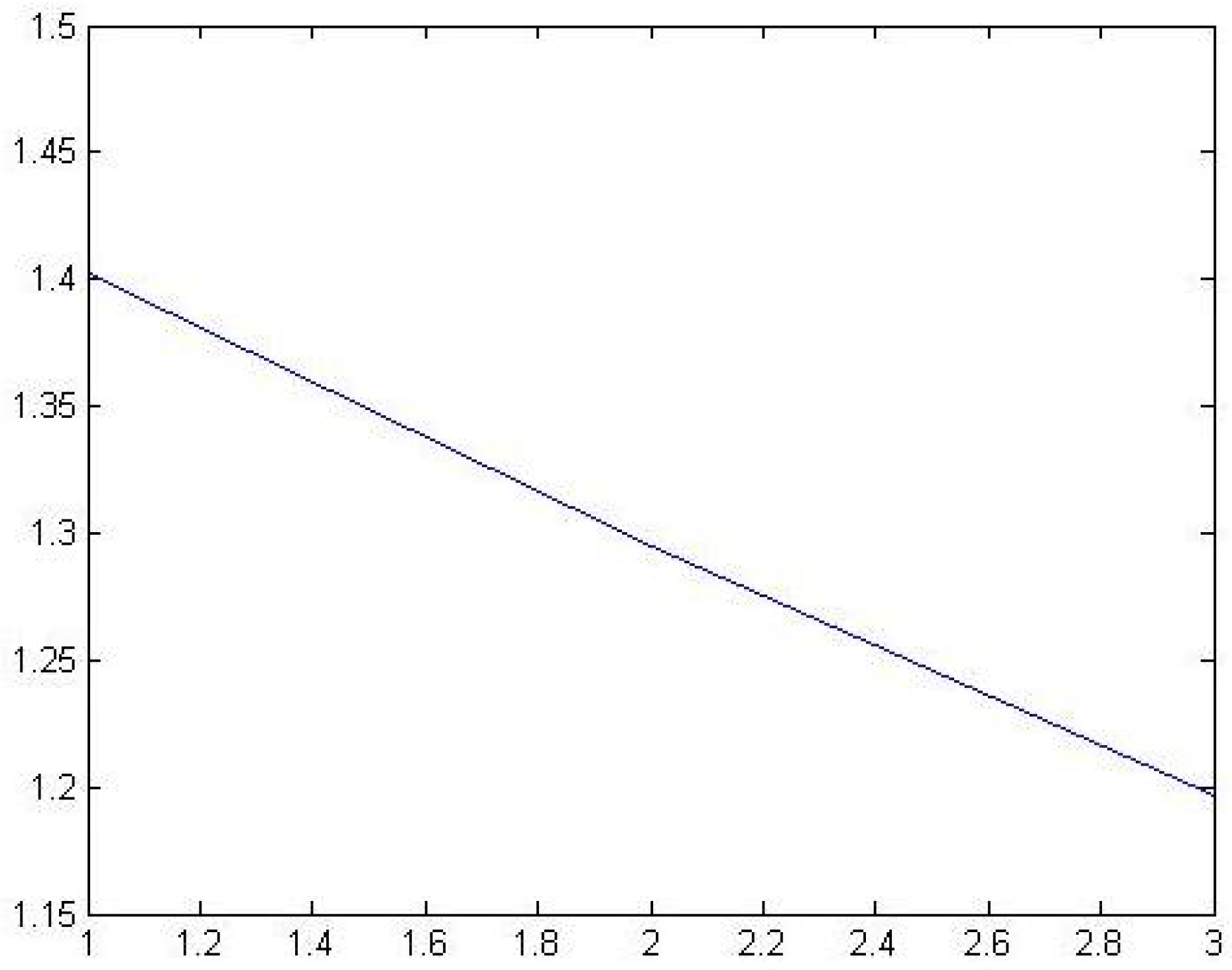
Theorem 1.
Figure 1.
The approximation of the average solution of state equation.
Proof.
The general term of the average solution given by (6) is alternated and decreases in absolute value towards zero, so this series is convergent (d’Alembert’s theorem). □
Moreover, suppose that the sensors provide some punctual average observation at the points given by
where M is the number of observation sensors.
We suppose that the available data are continuous-time averaged observations of the pollutant concentration at each of these M observation points.
Suppose we do not know the parameters of In the counterpart, we have at our disposal at M points , or the time history, as time t varies in the time interval of the average pollutant concentration
Let us define the operator B between and
where
and where is the average calculated observation corresponding to the parameter .
Let be the given averaged observation vector defined on the interval [0,T]. Then, we find such that
with .
Then, we define for that the cost function
where denotes the norm of H.
We take
where is the matrix.
The minimum of (11) is characterized by , so we have
We essentially suppose that B is one-to-one. Then, since it is well-known that is strictly positive definite, exists such that
If denotes the n-th vector of the canonical basis of , the n-th component of is given by and , and is symmetric, then
where is defined by , and then
Remark 1.
We solve this equation using the gradient method.
4. Gradient Method (Iterative Method (See in Figure 2))
To solve the equation , since the matrix is symmetric, then the resolution of the system (15) is equivalent to the minimization of for all w on .
Figure 2.
Error of the gradient relative to the number of iterations.
However, gradient methods are based on the fact that, if we give the vector of controls as , then the cost function and its gradient are obtained by solving the following two systems of equations by the decomposition method for, respectively, the state and the adjoint state q:
and
with , where is the average of with .
Lemma 1.
The components of the gradient of J are given by
where is the average of q with σ (see in Figure 3).
Figure 3.
The approximation of the average solution of adjoint state equation.
Proof.
We take the derivative following the direction ; then,
and then we have since
and since then
and since , then
and then grad J =. □
5. Average Solution to the Heat Equation with an Unknown Parameter
If we have
then the average solution, denoted , is
and then
In the same way, we calculate the average adjoint state, denoted :
Remark 2.
The average solution is also well-defined (see Theorem 1).
We deduce the components of the average gradient:
Now, we give two positive parameters, and , and we obtain:
If stop,
then
else, we repeat the calculation.
6. Numerical Application
To calculate the average solution , we take t and we can write this in the form
We take in (4), , , , for .
We calculate by solving Equation (4), and we calculate , by solving Equation (5). To calculate we use Equation (7), and we take to calculate the approximate average solution. Then, we find these results at .
To make the graph of the norm of the gradient vector with and , we find the control
7. Conclusions and Perspectives
The method of decomposing the solution to the system in a series with respect to the “sigma” parameter (reaction coefficient) allowed us to transfer the problem to a series of simple problems (independent of sigma). Using an iterative method, we calculated the components of the series using the calculation of the state and the obtained adjoint state of the system. The calculation of the average sentinel requires the resolution of a very large linear system (not recommended for numerical calculations), which made us think of an indirect method (optimization method). In addition, the calculation of the adjoint state allows the components of the gradient vector to be calculated. This new idea led to surprising results, meaning we could demonstrate the convergence of the series in a numerical way. It is believed that this new idea can be applied in several areas, including physical problems, wave problems, acoustics, bilinear control, inverse problems of determining stiffness coefficients, and topological degree techniques.
Author Contributions
Writing—original draft, H.S.; Writing—review & editing, A.A.; Supervision, I.R. All authors have read and agreed to the published version of the manuscript.
Funding
This work was supported by the Directorate-General for Scientific Research and Technological Development (DGRSDT).
Institutional Review Board Statement
The authors reveal that there are no ethical problems in the production of this paper.
Informed Consent Statement
The authors want to publish this paper in this journal.
Data Availability Statement
This paper does not use data or materials.
Acknowledgments
The authors are grateful to the reviewers for their valuable and insightful comments.
Conflicts of Interest
The authors declare that they have no competing interests.
References
- Kernévez, J.P. The Sentinel Method and Its Applications to Environmental Pollution Problems; CRC Mathematical Modelling Series; CRC Press: Boca Raton, FL, USA, 1997. [Google Scholar]
- Abdelhamid, A.; Chafia, L.; Abdelhak, H. Identification problem of a fractional thermoelastic deformation system with incomplete data: A sentinel method. Nonlinear Stud. 2022, 29, 399–410. [Google Scholar]
- Elhamza, B.; Hafdallah, A. Identification of the bulk modulus coefficient in the acoustic equation from boundary observation: A sentinel method. Bound Value Probl. 2023, 2023, 23. [Google Scholar] [CrossRef]
- Zuazua, E. Averaged control. Automatica 2014, 50, 3077–3087. [Google Scholar] [CrossRef]
- Fursikov, A.V. Properties of solutions of some extremal problems connected with the Navier-Stokes system. Math. USSR-Sb. 1983, 46, 323–351. [Google Scholar] [CrossRef]
- Lions, J.L. Some notions in the analysis and control of incomplete data systems. In Proceedings of the 11th Congress on Differential Equations and Applications, Kyoto, Japan, 21–29 August 1990; pp. 43–54. [Google Scholar]
- Elhamza, B. Hafdallah: Identification of the potential coefficient in the wave equation with incomplete data: A sentinel method. Russ. Math. 2022, 2022, 113–122. [Google Scholar] [CrossRef]
- Raore, A.; Mampassi, B.; Saley, B. A Numerical Approach of the sentinel method for distributed parameter systems. Open Math. 2007, 5, 751–763. [Google Scholar] [CrossRef]
- Selatnia, H.; Berhail, A.; Ayadi, A. Average Sentinel for a Heat Equation with Incomplete Data. J. Appl. Comput. Math. 2018, 7, 2. [Google Scholar] [CrossRef]
- Fursikov, A.V.; Imanuvilov, O.Y. Controllability of Evolution Equations; Séoul National University: Seoul, Republic of Korea, 1996. [Google Scholar]
- Lions, J.L. Contrôle Optimal de Systèmes Gouvernés par des Equations aux Dérivées Partielles; Dunod: Paris, France, 1968. [Google Scholar]
- Lions, J.L.; Bensoussan, A.; Glowinski, R. Méthode de Décomposition Appliquée au Contrôle Optimal de Systèmes Distribués. In Proceedings of the 5th IFIP Conference on Optimization Techniques, Rome, Italy, 7–11 May 1973; Lecture Notes in Computer Science. Springer: Berlin, Germany, 1973; Volume 5. [Google Scholar]
- Chavent, G. Generalized sentinels de ned via least squares. Appl. Math. Optim. 1993, 31, 189–218. [Google Scholar] [CrossRef][Green Version]
- Lions, J.L. Sentinelles Pour les Systémes Distribués à Données Incomplètes; Masson, RMA: Paris, France, 1992; Volume 21. [Google Scholar]
- Lions, J.L. Contrôlabilité exacte, perturbations et stabilisation de systèmes distribués. In Contrôlabilité Exacte, Recherches en Mathématiques Appliquéesl; Masson: Paris, France, 1988; Volume 8. [Google Scholar]
- Massengo, G.; Nakoulima, O. Sentinels with given sensitivity. Eur. J. Appl. Math. 2008, 19, 21–40. [Google Scholar] [CrossRef]
- Merabet, A.; Ayadi, A.; Omrane, A. Detection of pollution terms in nonlinear second order wave systems. Int. J. Parallel Emergent Distrib. Syst. 2019, 34, 13–20. [Google Scholar] [CrossRef]
- Nakoulima, O. Optimal control for distribute systems subject to null controllability. Application to discrimiting sentinels. Esaim Control Optim. Calc. Var. 2007, 13, 623–638. [Google Scholar] [CrossRef]
Disclaimer/Publisher’s Note: The statements, opinions and data contained in all publications are solely those of the individual author(s) and contributor(s) and not of MDPI and/or the editor(s). MDPI and/or the editor(s) disclaim responsibility for any injury to people or property resulting from any ideas, methods, instructions or products referred to in the content. |
© 2024 by the authors. Licensee MDPI, Basel, Switzerland. This article is an open access article distributed under the terms and conditions of the Creative Commons Attribution (CC BY) license (https://creativecommons.org/licenses/by/4.0/).