Abstract
The paper is a continuation and completion of the paper Bruno, A.D.; Azimov, A.A. Parametric Expansions of an Algebraic Variety Near Its Singularities. Axioms 2023, 5, 469, where we calculated parametric expansions of the three-dimensional algebraic manifold , which appeared in theoretical physics, near its 3 singular points and near its one line of singular points. For that we used algorithms of Nonlinear Analysis: extraction of truncated polynomials, using the Newton polyhedron, their power transformations and Formal Generalized Implicit Function Theorem. Here we calculate parametric expansions of the manifold near its one more singular point, near two curves of singular points and near infinity. Here we use 3 new things: (1) computation in algebraic extension of the field of rational numbers, (2) expansions near a curve of singular points and (3) calculation of branches near infinity.
MSC:
41A60
1. Introduction
Here we continue and conclude the paper [1]. There, in Sections 1–5, we proposed a new method for solving the polynomial equation
near a singular point or curve of singular points of the polynomial f. In Sections 6–10, this method was applied to compute the solutions to such a 12th degree equation with that originated in theoretical physics. This new method is based on:
- Newton’s polyhedron to isolate the truncated equations,
- Power transformations to simplify those equations, and
- Formal Generalized Implicit Function Theorem to obtain solutions in the form of power expansions whose coefficients are rational functions of the parameters. Computer algebra is used in these calculations.
Newton’s polyhedron is a multidimensional generalization of Newton’s polygon (see [2,3,4,5,6,7]). Power transformations are a generalization of the sigma process used previously to resolve singularities of algebraic manifolds (see [8,9,10]). Algorithms for computing power transformations were proposed in [11]. The resolution of the singularity is done step-by-step until we come to the situation with a truncated equation containing a polynomial multiplier of degree one. If the roots of this multiplier are parameterized, the roots of the whole polynomial are obtained as a power expansion using a Generalized Implicit Function Theorem (Theorem 1 of [1]). All these are an application to algebraic equations of the general theory of Nonlinear Analysis [12], which is also suitable for differential equations. For its applications to systems of partial derivative equations, see [13].
According to [1] and [12] (Section 2) computational steps are the following:
- Step 1.
- Introduction of local coordinates. For coordinates and singular point , they are , i.e., , .
- Step 2.
- Writing the initial polynomial in local coordinatesHere , , are real or complex coefficients, the sum has not similar terms, the set , is called as support of the sum . Here . Let the support consists of vectors .
- Step 3.
- The Newton polyhedron is computating as the convex hull of the support :The boundary of the polyhedron consists from its generalized faces , where d is dimension, , and j is a number of the face . Each face corresponds to its truncated polynomialand the normal cone , consisting of all normals to the face , which are external to the polyhedron . For their computation we use the PolyhedralSets package of the computer algebra system (CAS) Maple. In the steps below . Then is two dimensional face and normal cone is a ray, spanned by external normal to the face .
- Step 4.
- We select faces with normal and corresponding truncated polynomials .
- Step 5.
- For each selected truncated polynomial , we compute corresponding power transformationwhere is an unimodular matrix, such thatwith integral l.
- Step 6.
- If the curve has parametrizationthen it is obtained with the algcurves package from the CAS Maple. In that case we make the power transformation (2) in the full polynomial (1) and write it aswith some natural m. Here polynomials are computed by the command coeff(T,z[k],m) in CAS Maple. Here from (3).
- Step 7.
- If , we make the substitutioninto the polynomial , obtain function , apply to the equation the Formal Generalized Implicit Function Theorem 1 [1] and get the parametric expansion
- Step 8.
- We compute several terms of expansion (5), substitute them into (4). The result is substituted in power transformation (2), and we obtain parametric expansion of Y in power series of with coefficients which are rational functions of t.If , we continue computation with new Newton polyhedron etc.
The method is new, with parts: the Newton polyhedron , polyhedron’s faces , polyhedron graph, normal cones and power transformations (2) were proposed by the first author beginning 1962. Early such objects he calculated manually, but now there are programs for that.
In [1], this theory was applied to a problem arises in the study of Ricci flows (see [14,15,16,17,18,19,20,21,22]). The Ricci flows describe the evolution of Einstein’s metrics on a variety. The equations of the normalized Ricci flow are reduced to a system of two differential equations with three parameters: , and :
here, and are certain given functions.
The singular points of this system are associated with the invariant Einstein’s metrics. At the singular (stationary) point , , system (6) has two eigenvalues, and . If at least one of them is equal to zero, then the singular (stationary) point , is said to be degenerate. It was proved in [14,15,16,17,18,19,20,21,22] that the set of the values of the parameters , , , in which system (6) has at least one degenerate singular point, is described by all solutions of the equation
where , , are elementary symmetric polynomials, equal, respectively, to
Here Q is different from Q’s in Steps 2 and 3, but the sign means only a new notation.
Hence the polynomial has degree 12. In [23], for symmetry reasons, the coordinates were changed to the coordinates by the linear transformation
The resulting polynomial is
and has degree 12 again.
Definition 1.
Let be some polynomial, where . A point of the set is called the singular point of the k-order, if all partial derivatives of the polynomial with respect to turn into zero at this point, up to and including the k-th order derivatives, and at least one partial derivative of order is nonzero.
In [23], all singular points of the variety in coordinates were found. The five points of the third order are:
| Name | Coordinates |
three points of the second order
| Name | Coordinates |
and three more algebraic curves of singular points of the first order:
The points , and are of the same type; they pass into each other when rotated in the plane by an angle , just as all points , , . The curves , , correspond to two more curves of the same type. Therefore, it is sufficient to study the variety in the neighborhood of points , , , and curves , and . Moreover, in [23] there were computed sections of the variety by planes , and was shown that in finite part of the space the variety consists of two dimensional branches , , , , , divided into parts , with boundaries at the plane .
In the paper [24], three variants of the global parametrization of the variety were proposed. These parametrizations were computed using the parametric description of the discriminant set of a monic cubic polynomial [25] and can be written in radical form [26]. Such a global description of the variety cannot provide an adequate picture of the structure in the vicinity of its singular points.
In [1], parametric expansions of the variety near the singular points (Section 7), (Section 8), (Section 8), (Section 10) and near the line of singular points (Section 9) were computed. Here these expansions are computed near the singular point (Section 2), near the curves of singular points (Section 3) and (Section 4), and near infinity (Section 5). Together they cover a wide range of cases. The following tactic has developed: if the truncated equation contains linear multipliers, they are used to do a linear transformation of the coordinates followed by the computation of Newton’s polyhedron; and if they are nonlinear, a power transformation of the coordinates is done. To understand the present article it is necessary a knowledge with papers [1] (open access), [23] and the book [27].
2. The Structure of the Manifold near the Singular Point
2.1. Preliminary Computations
Near the point we introduce local coordinates :
Then, from the polynomial in (7) we get a polynomial of degree 12.
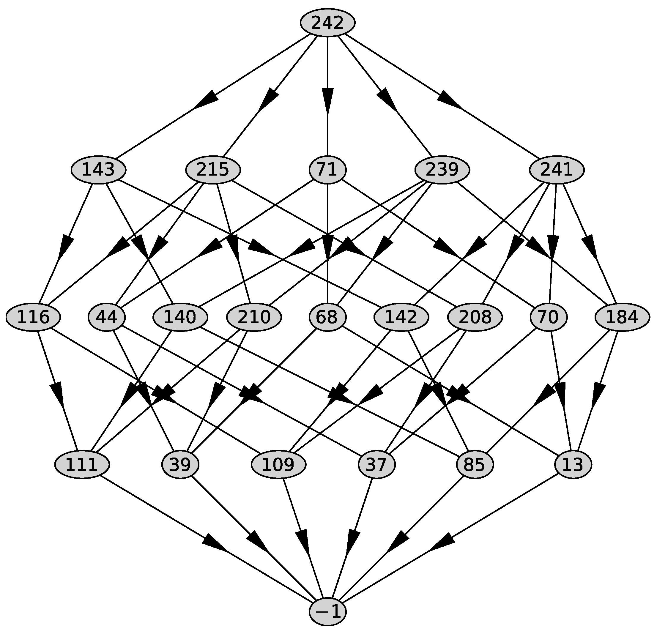
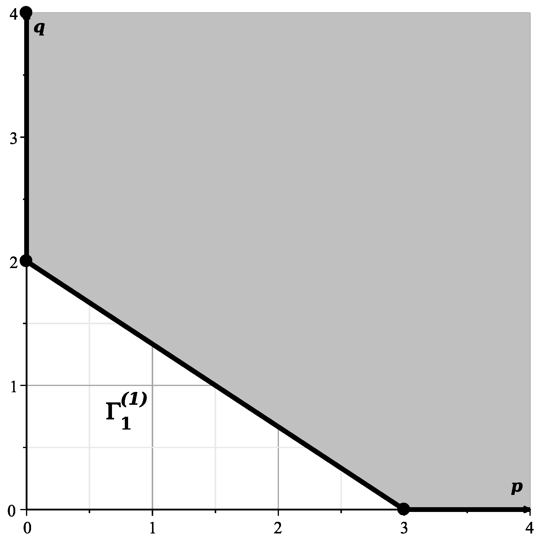
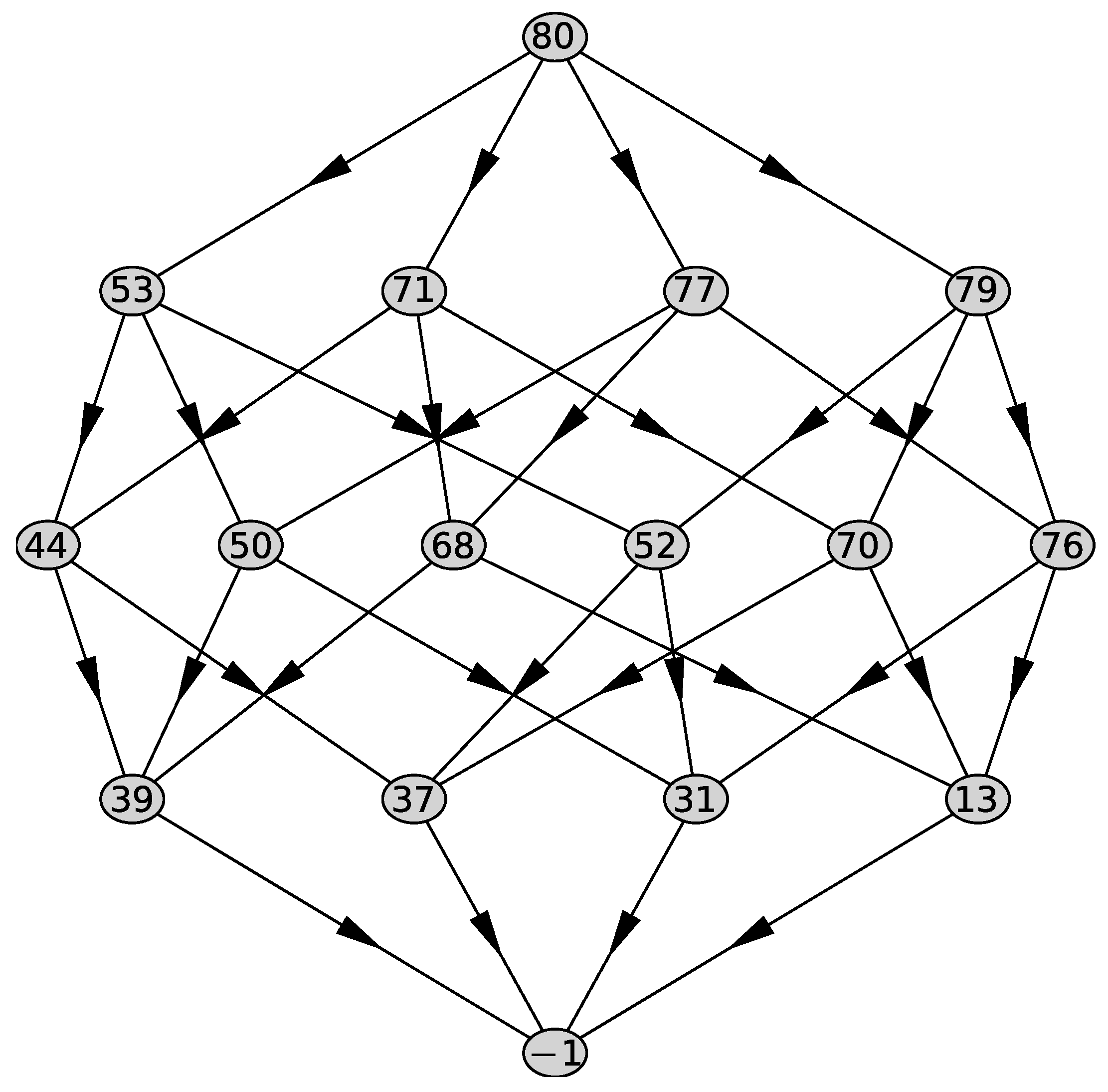
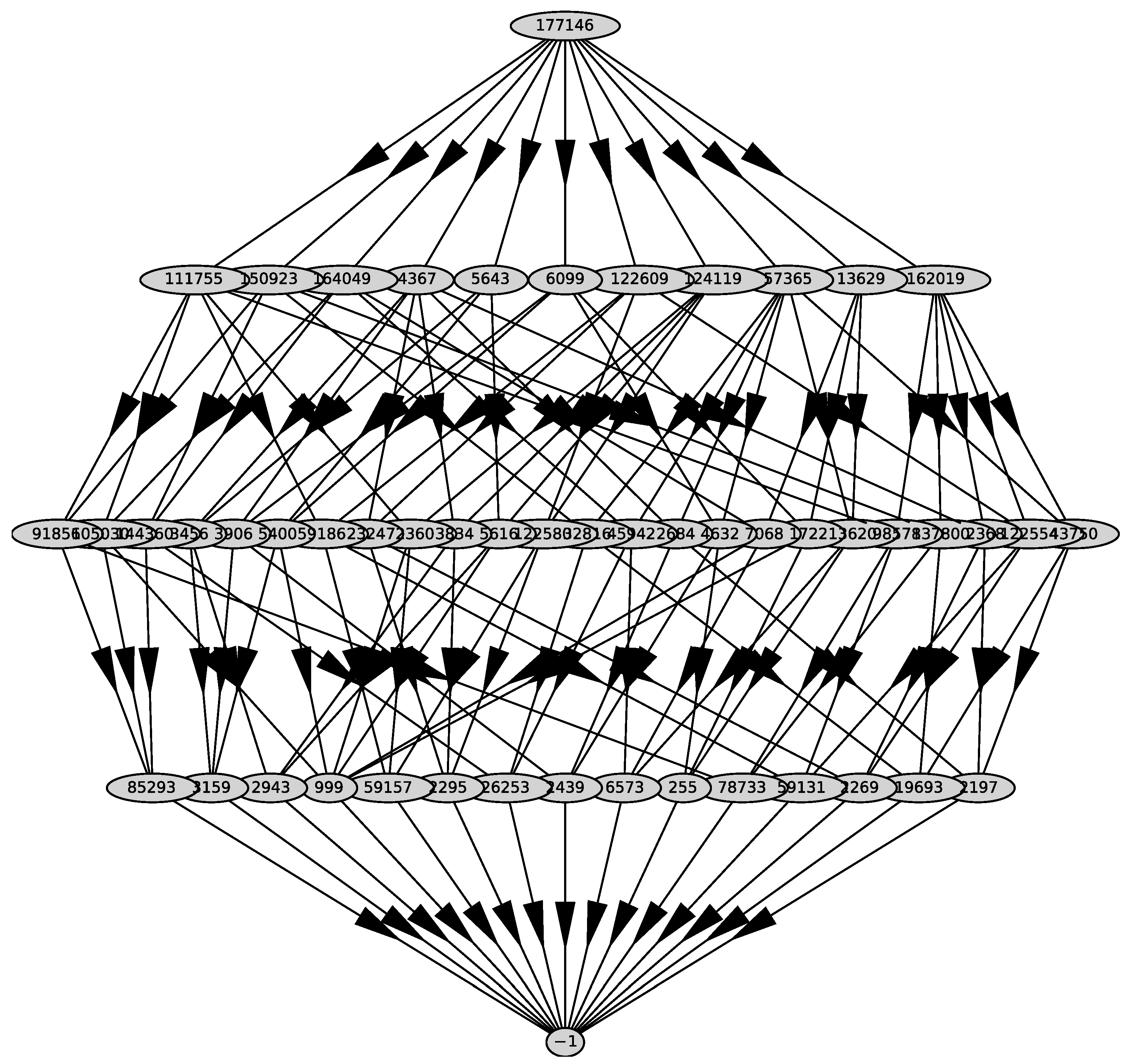
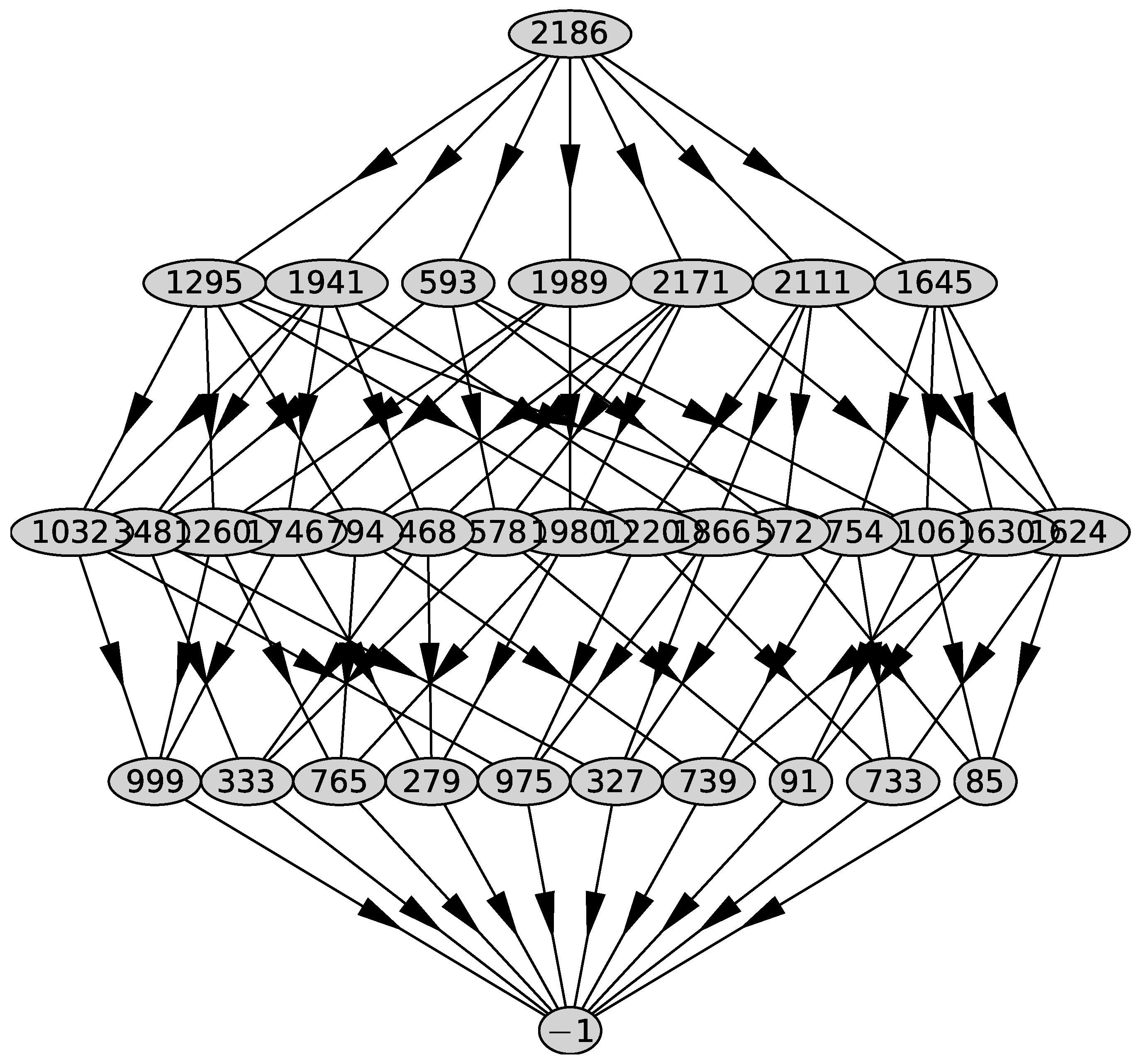
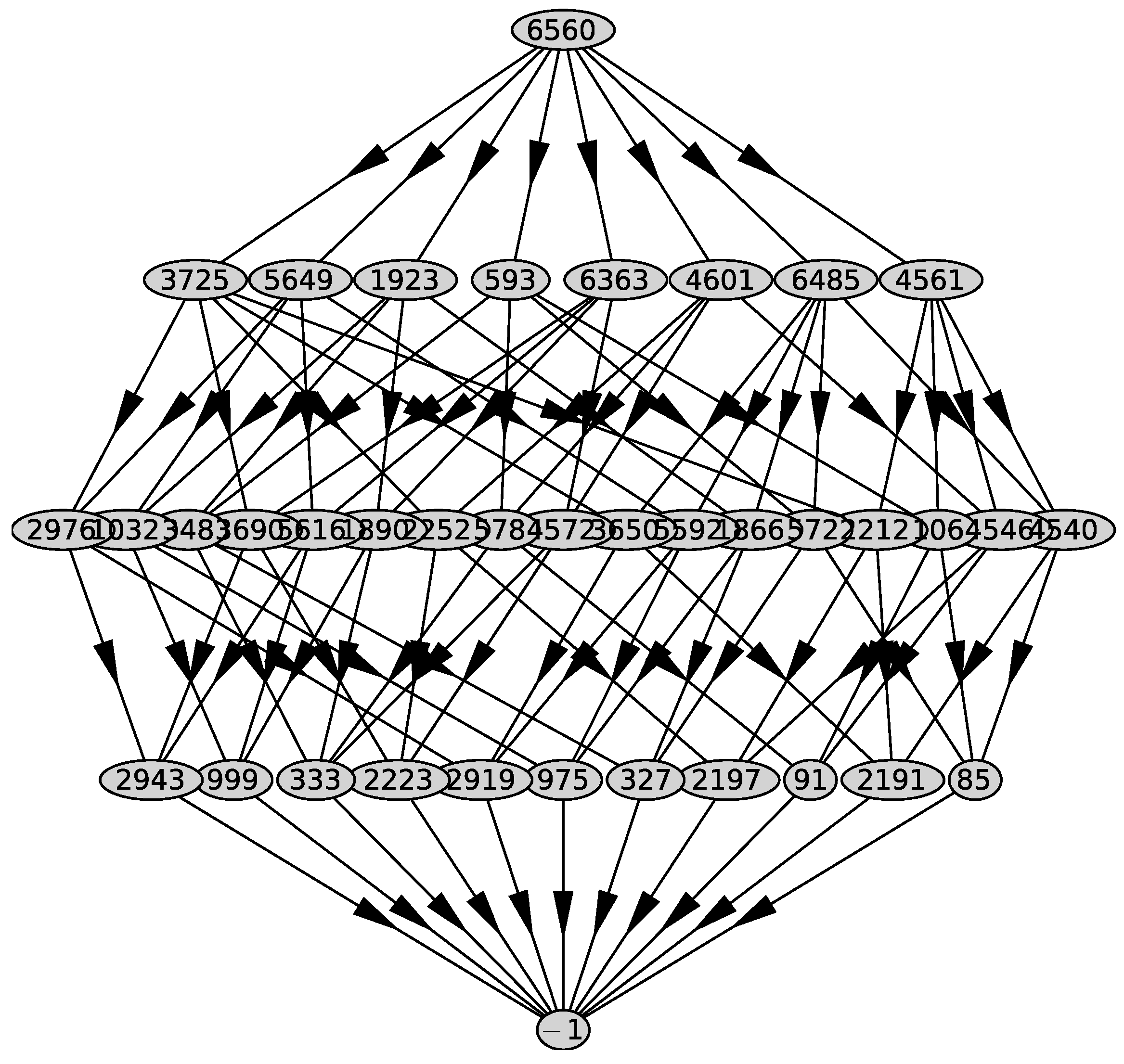
We compute the support of the polynomial , the Newton polyhedron , its faces and their external normals using the PolyhedralSets package of the computer algebra system (CAS) Maple 2021 [27]. We obtain 5 faces . The graph of the polyhedron is shown in Figure 1.
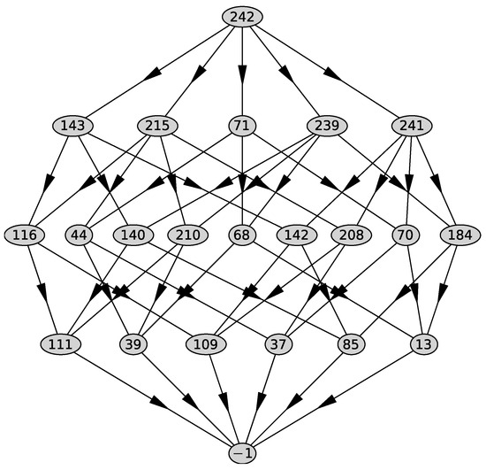
Figure 1.
Graph of the polyhedron .
In the top row—the whole polyhedron, in the next—all two-dimensional faces. Further down are the edges, then the vertices, and at the bottom is the empty set. The external normals to its two-dimensional faces are
Since we take the only normal that has all coordinates negative. This is . It corresponds to a truncated polynomial
The quadratic polynomial bracketed in (9) does not factorize in the field of rational numbers, but it does factorize in the extension of this field with . We get
We proceed according to [27]:
- >alpha := RootOf(y^2-3);
- >factor (f,alpha);
Now we do a linear substitution of the coordinates
Its inverse substitution is
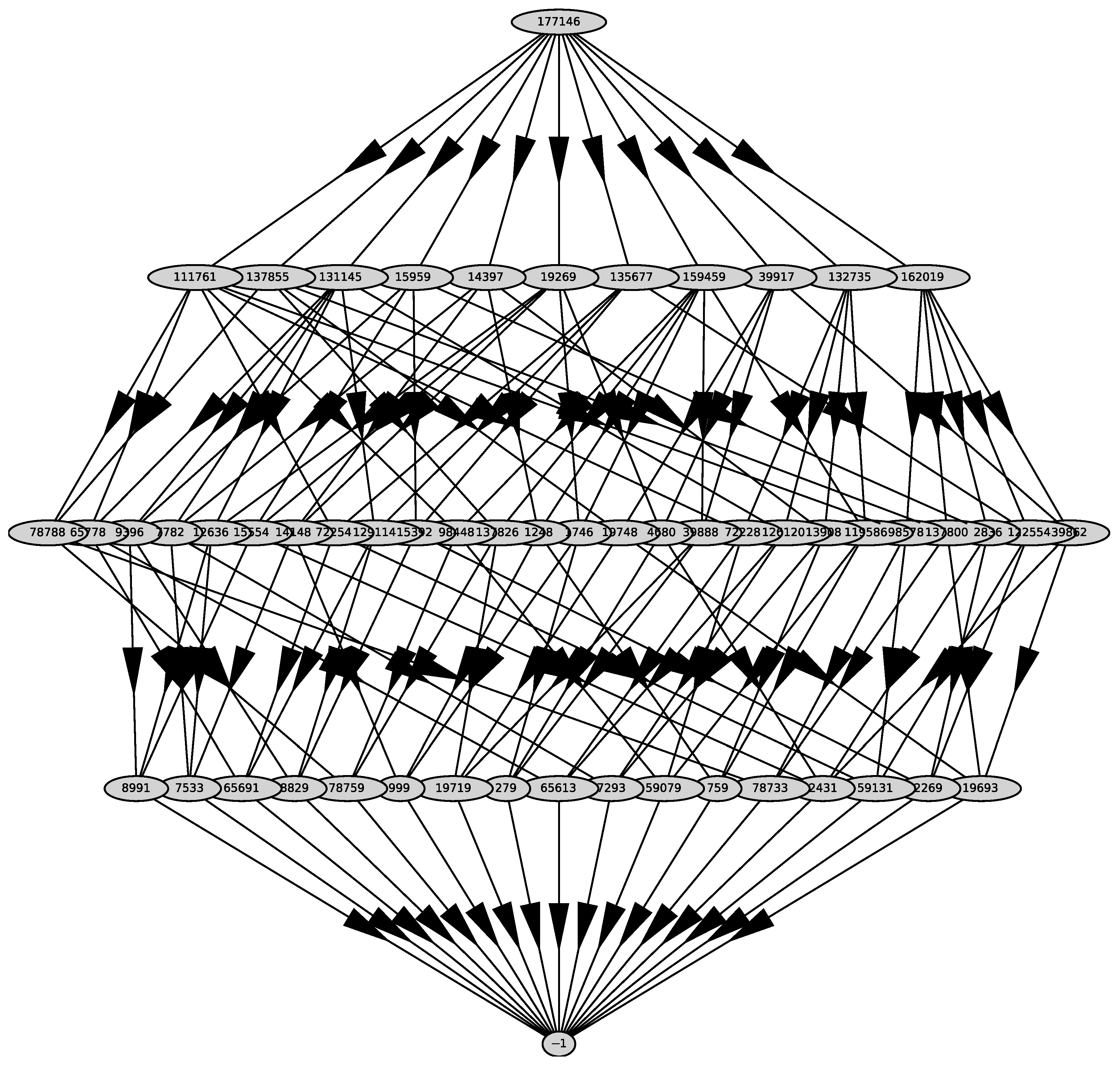
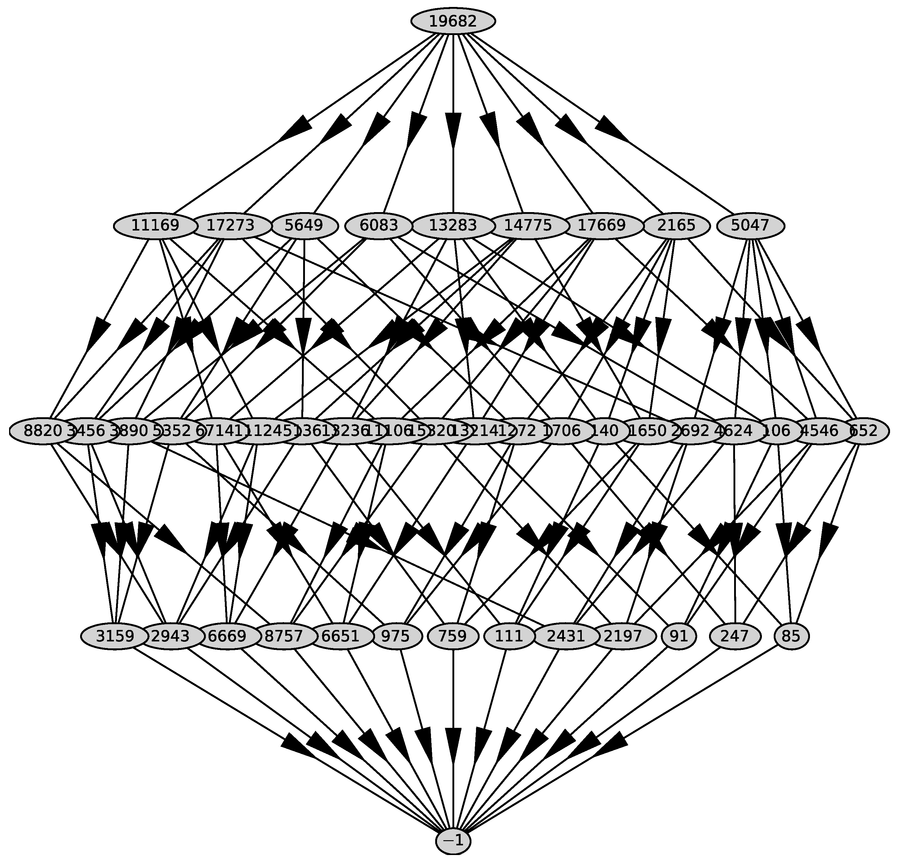
We substitute it into the polynomial and get the polynomial . For the polynomial , we compute Newton’s polyhedron . Its graph is shown in Figure 2. It has 11 two-dimensional faces with external normals

Figure 2.
Graph of the polyhedron .
We parse the first 4 of them that have 2 or 3 coordinates negative, dedicating a subsection to each of them. Below we use notation from Maple [27].
2.2. The Normal
The corresponding truncated polynomial is
where . Here and below “” number means truncated polynomial, corresponding to normal with written number j. According to [11], we compute the matrix such that . Since , then we do a power transformation
We get after factorization
where . The large polynomial in the parentheses is denoted by
Consider the curve It has intersections with the axes: It is a curve of genus 0, with one singular point
and parameterization
We simplify these expressions by transforming and obtaining
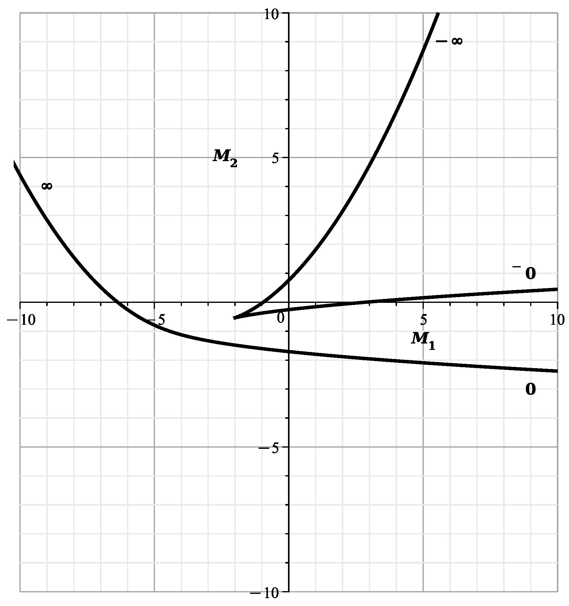
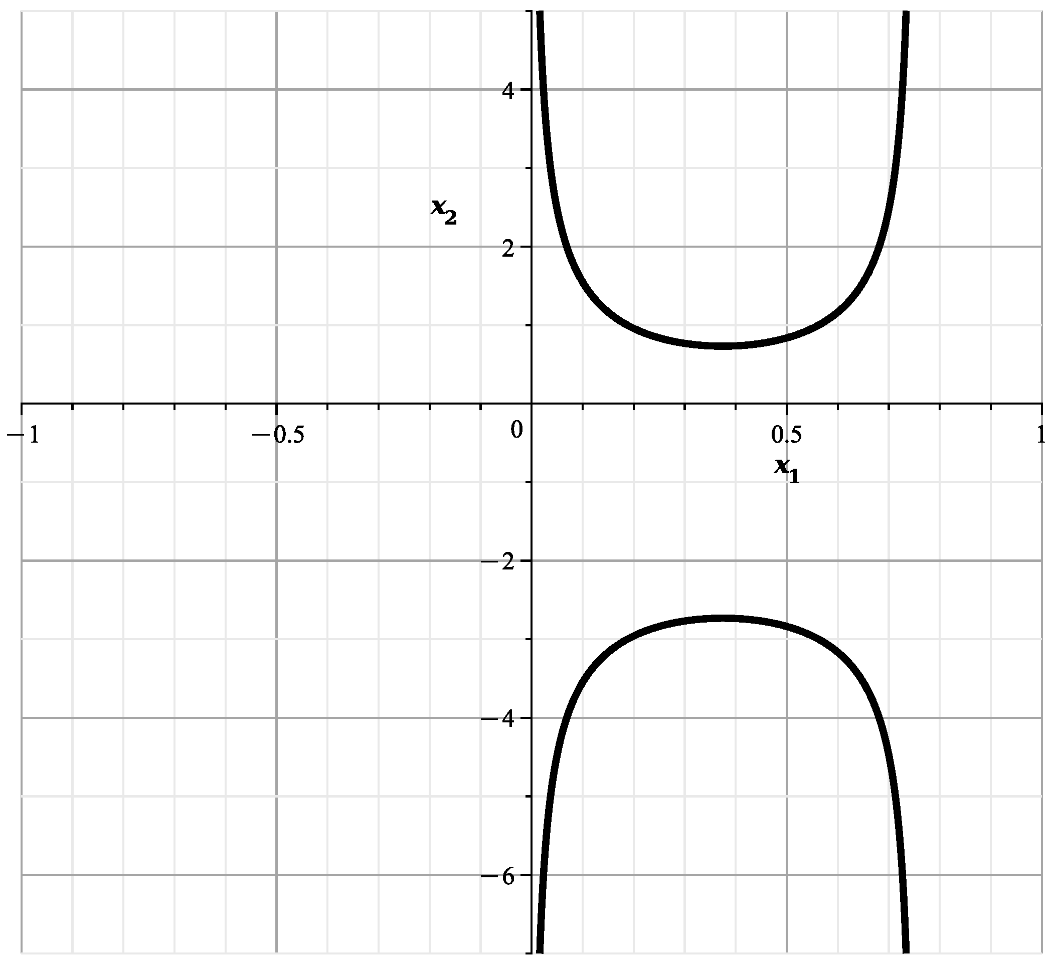
The curve is shown in Figure 3.

Figure 3.
Curve .
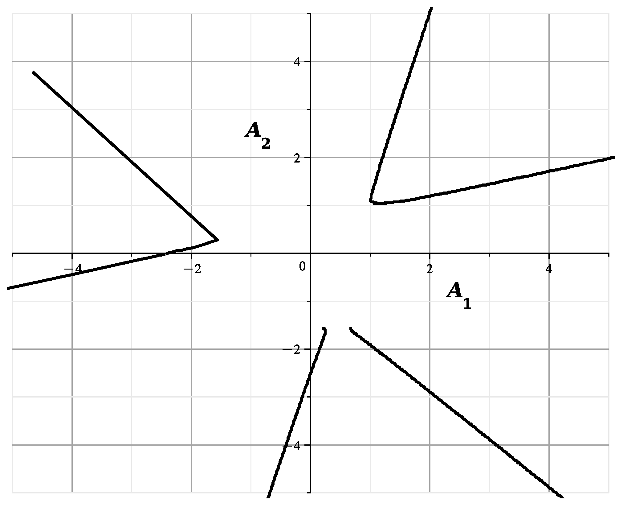
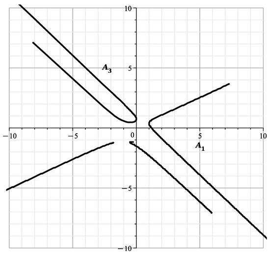
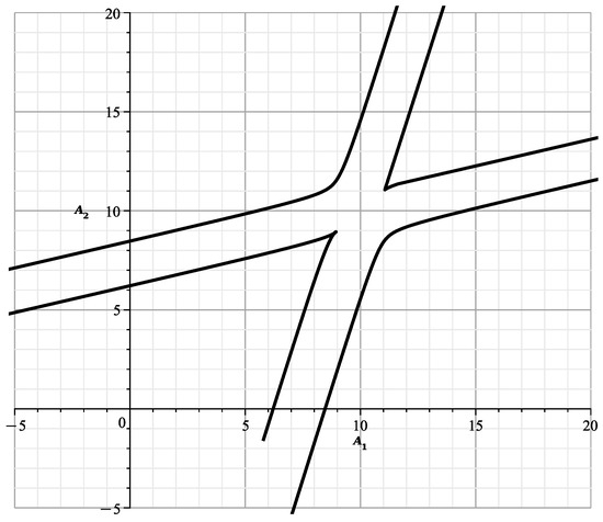
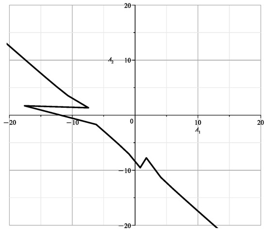
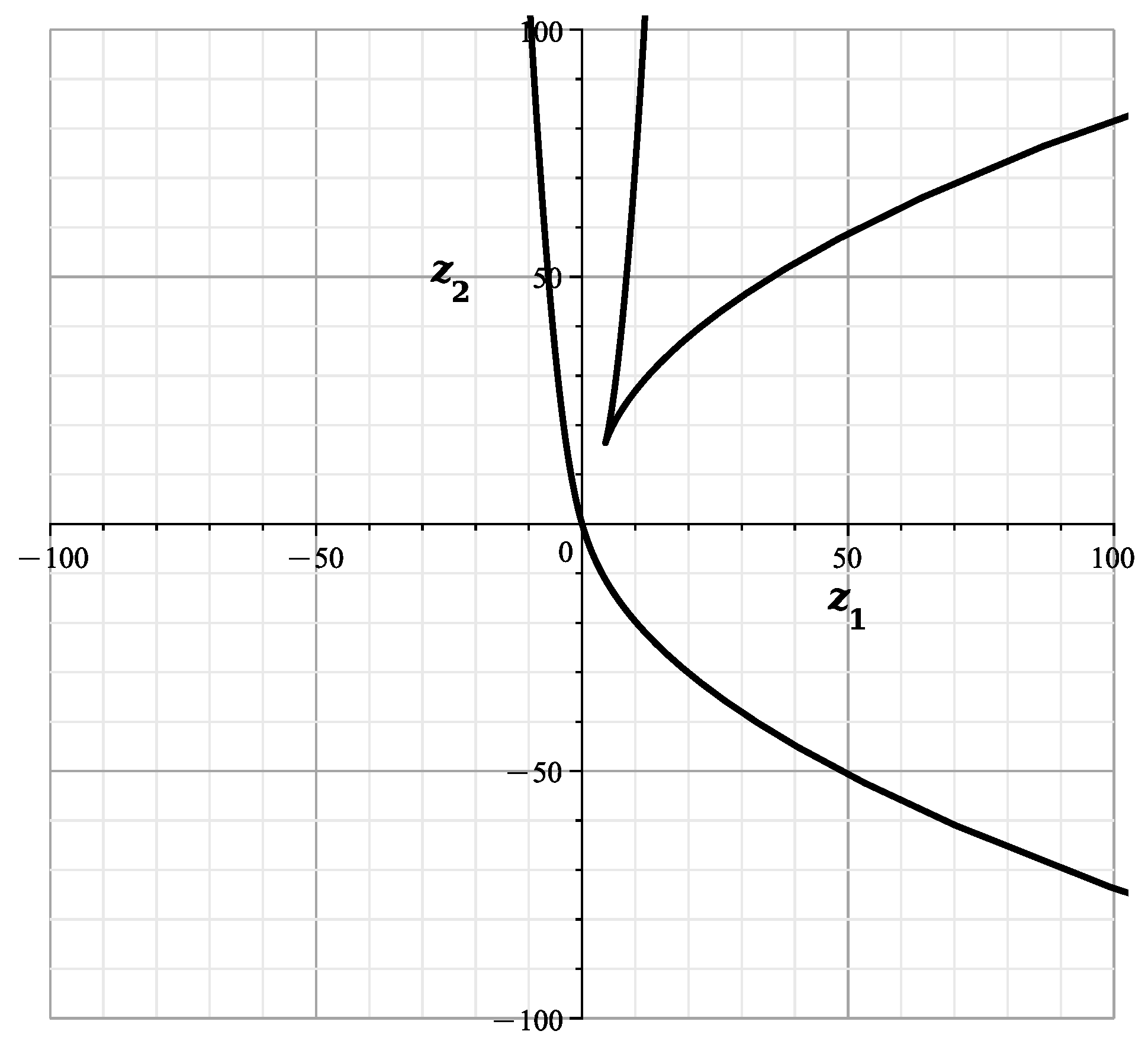
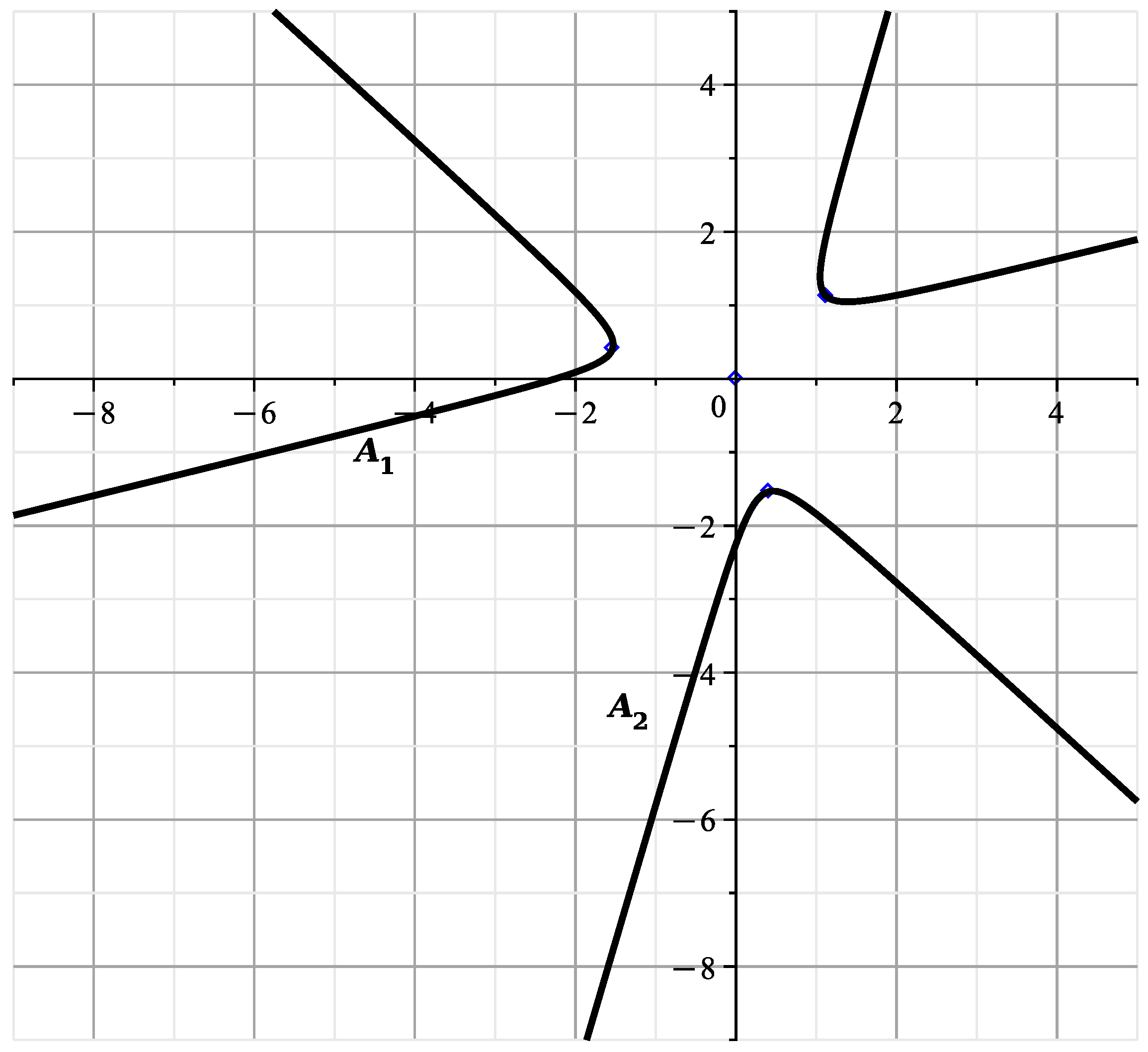
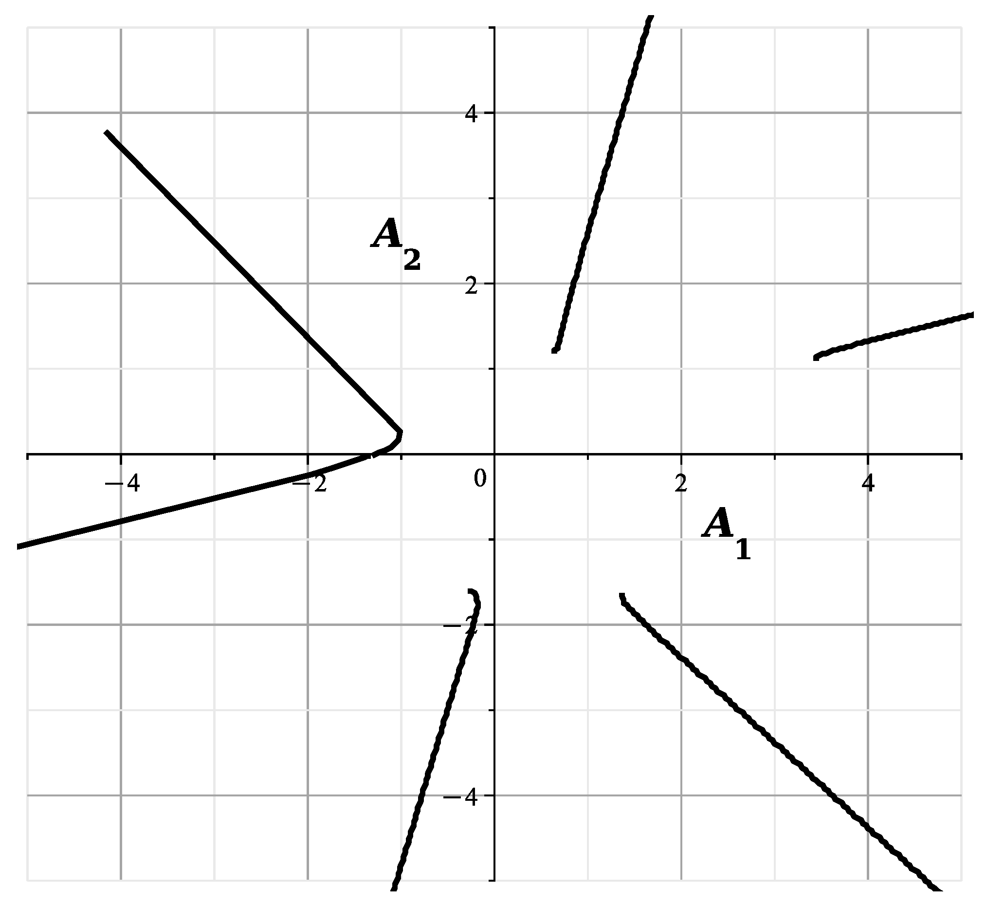
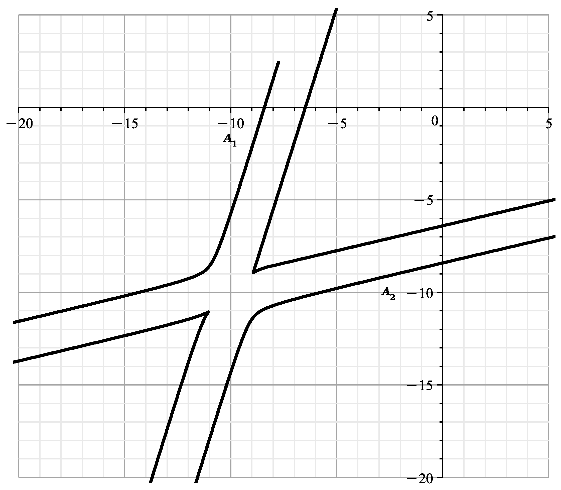
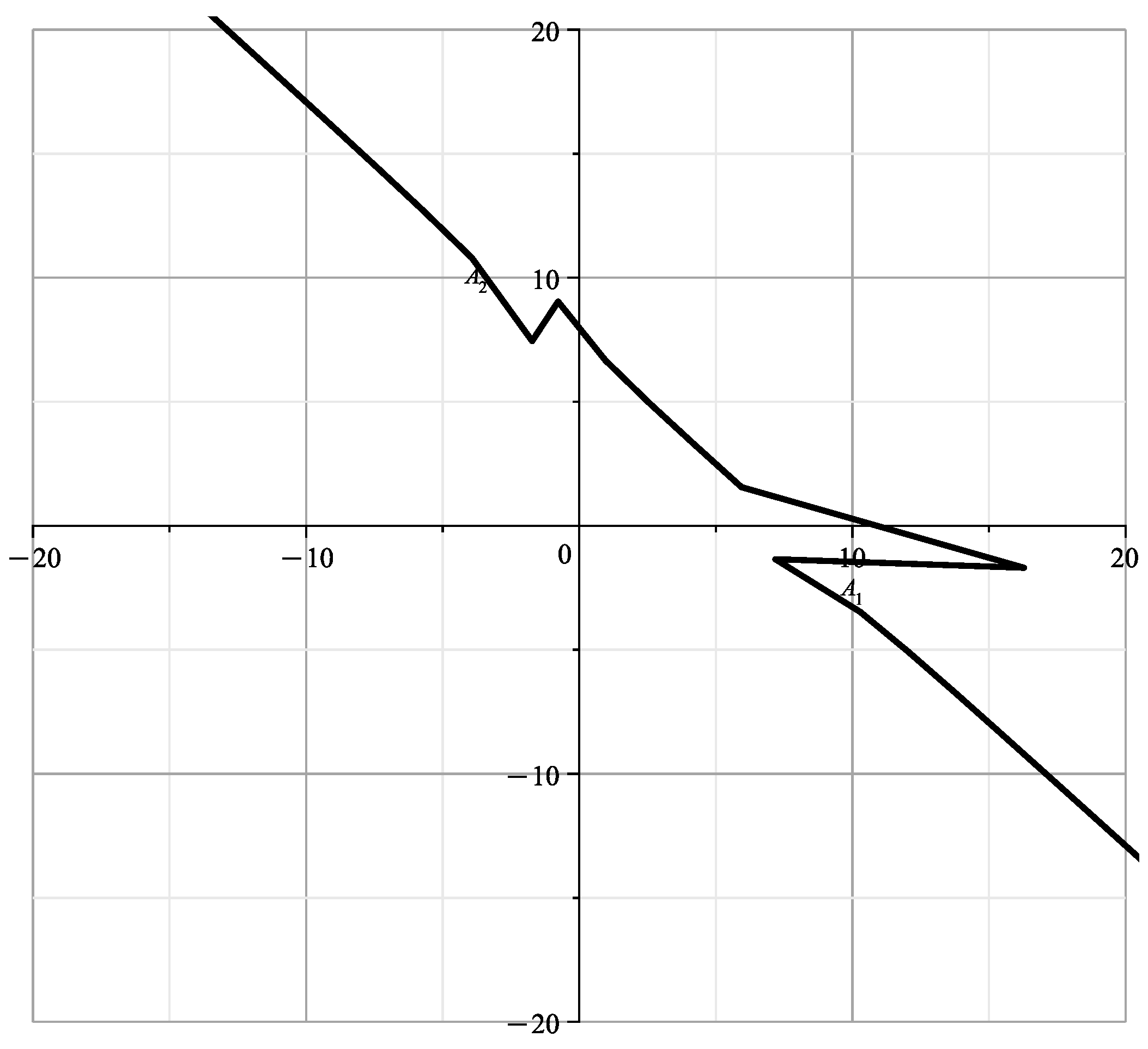
With fixed according to (8), (10) and (11) at the original coordinates , we obtain a curve
where , according to (12).
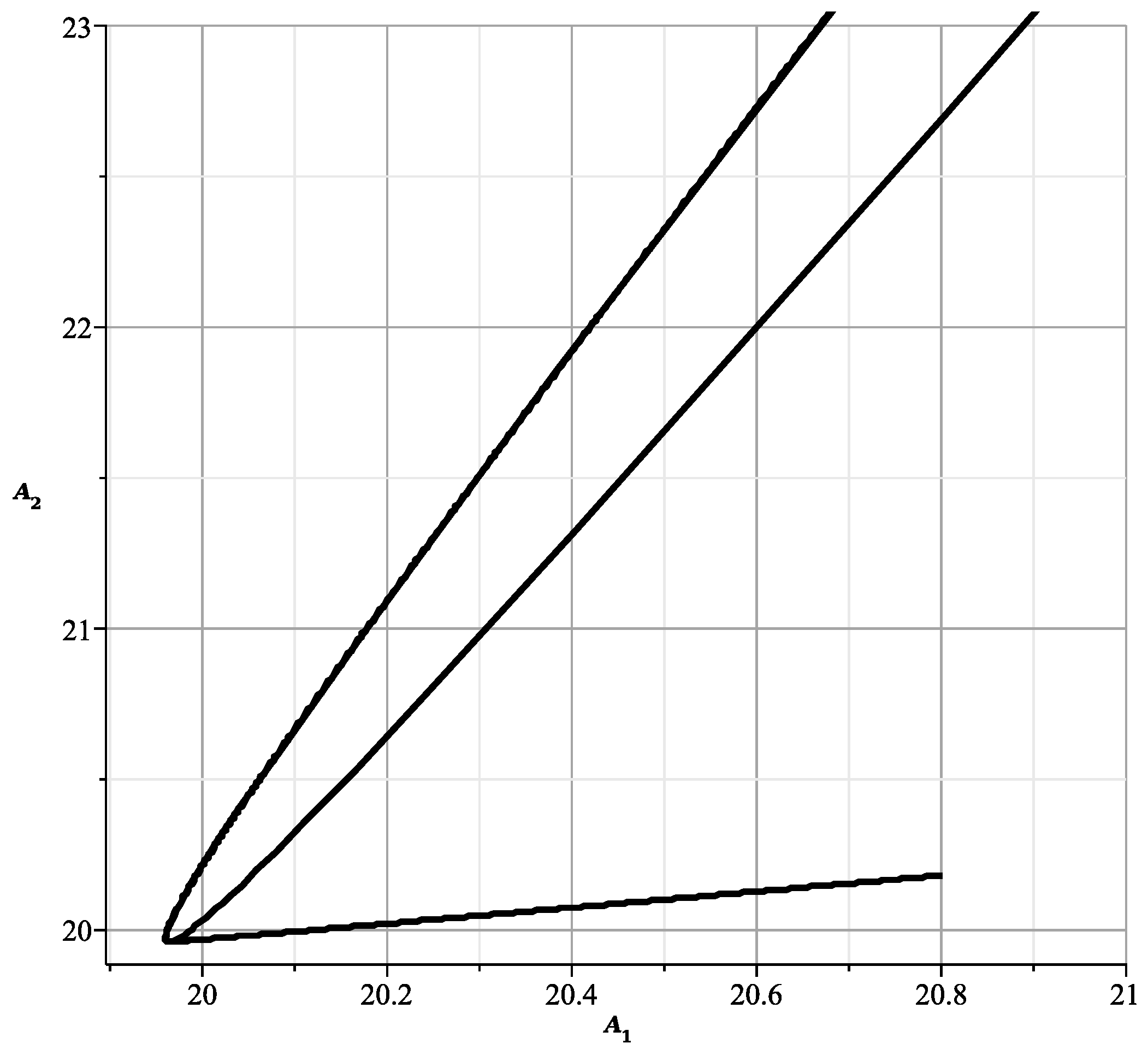
This curve is shown in Figure 4. This curve is similar to the curve of [23] (Figure 12) showing the cross-section of the variety at , with branches and .
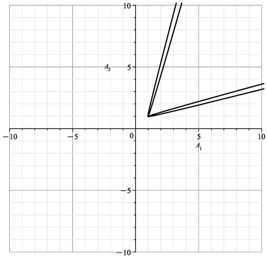
Figure 4.
Curve (14).
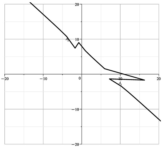
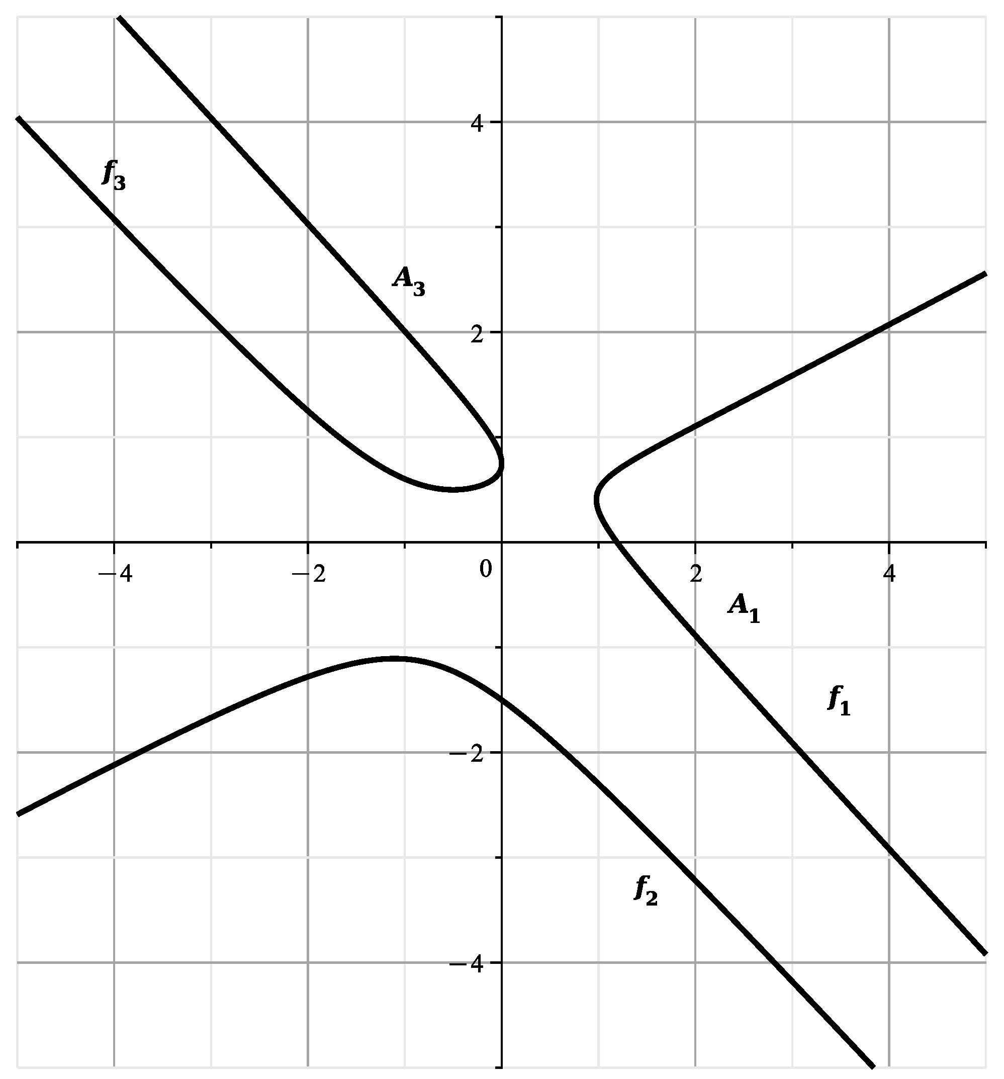
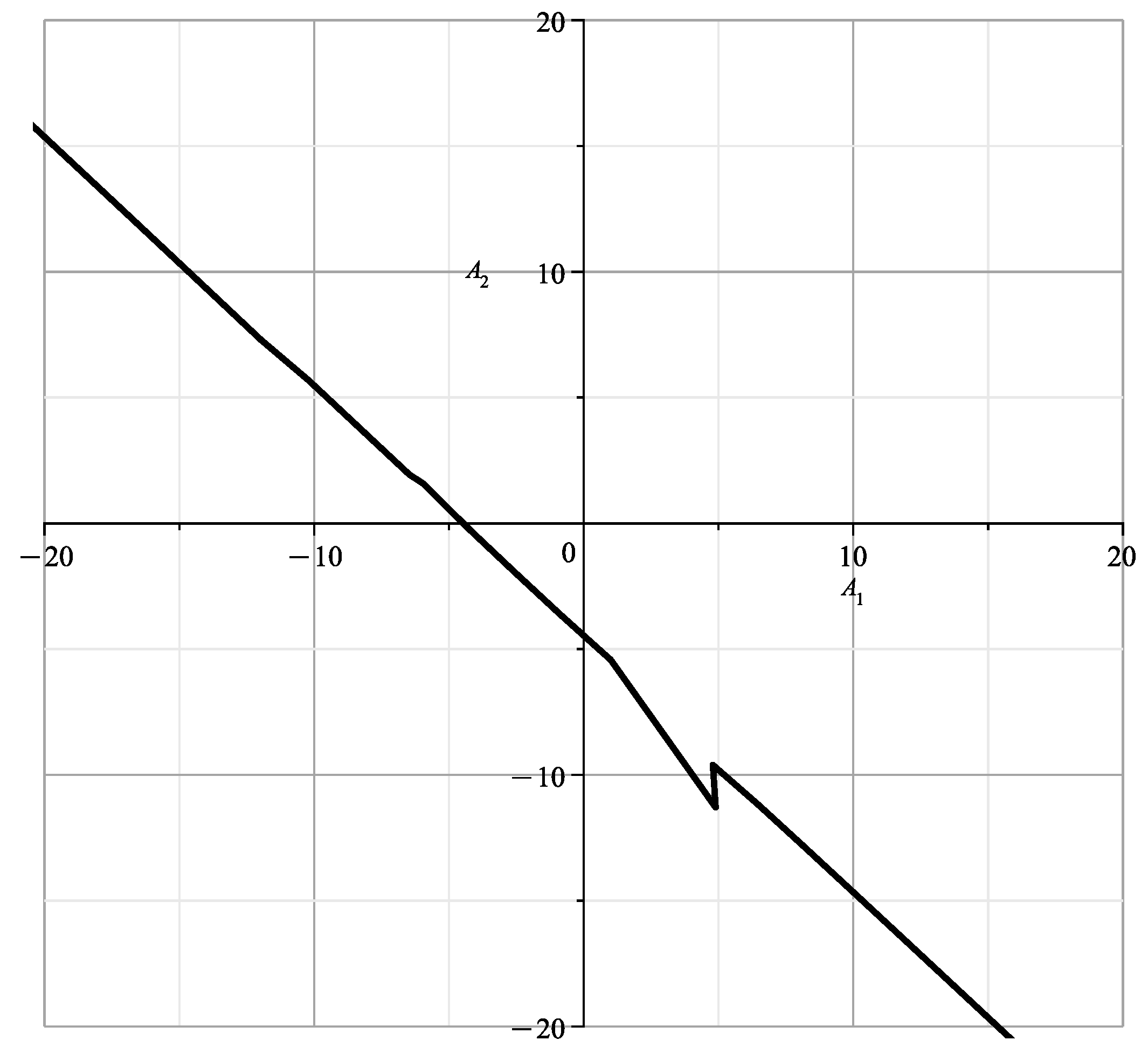
If , then , hence according to (13)
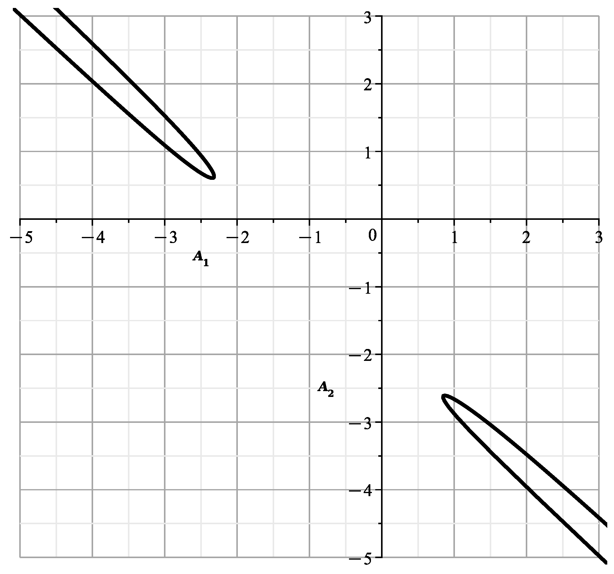
When , , the curve (15) is shown in Figure 5. It is similar to Figure 15 in [23], which shows the section of the variety at , with coinsiding branches and .
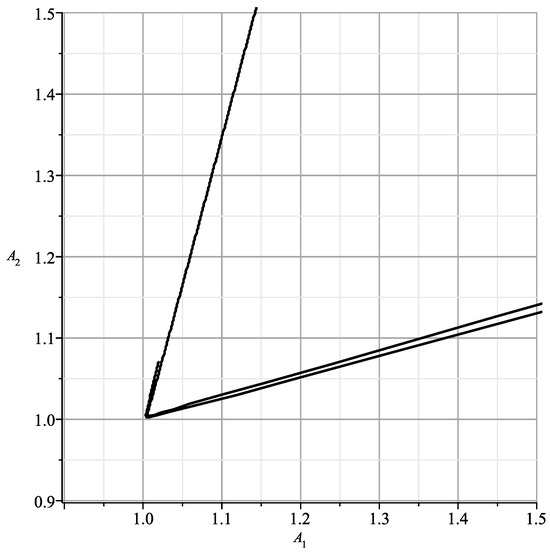
Figure 5.
Curve (15).
In fact, the parametric expansion of the variety can also be computed here. To do this, we substitute (11) into the polynomial and get the polynomial of Step 6
where polynomials are uniquelly determined and can be computed by the command coeff(T,z[k],m).
In it, according to (12), we make the substitution
We obtain that with coefficients depending on t via and . We apply Theorem 1 in [1] to the equation and obtain the expansion
2.3. The Normal
It corresponds to a truncated polynomial
Since it is linear on , its root is the -axis, i.e., , which we denote by N. This line N lies on the variety and through N it passes one of its branches, which in the first approximation has the form .
This is the straight line of [23] (Figure 3). In [23] (Figures 4–15), the points of the line N lie in the plane . Moreover, in Figure 6 , in Figures 8–11 , in Figures 4, 13 and 14 . According to (19), there are 3 singular points on the line N
In coordinates, they look like this:
i.e., they are points , and a point with on the curve of singular points. The structure of the variety near the point is dealt with in this Section, near the point was dealt with in Section 7 of [1], and in the next Section we will deal with the structure of the variety near the curve .
We can obtain an expansion of the variety near the line N. To do this, we substitute (10) in the polynomial and obtain the polynomial which we write as
where , polynomials. Thus according to (19)
According to [1] (Theorem 1), the equation has a solution
Going to the original coordinates, we get the expansion for with parameters and . It is valid everywhere except the neighborhoods of the points (20).
2.4. The Normal
It corresponds to a truncated polynomial
Let’s put
According to [11], we compute the unimodular matrix such that . Since , then we do a power transformation
We get
Let’s denote
The curve has genus 0, intersections with axes
parameterization
The singular points are reached at
The plot of the curve is shown in Figure 6:
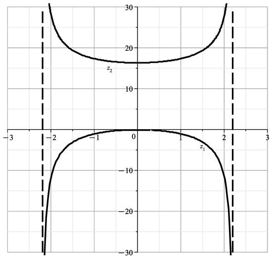
Figure 6.
Plot of the curve
If then,
This is the singular line of [23] (Figure 5), which is obtained from the singular line by rotating by an angle If , then according to (25) and
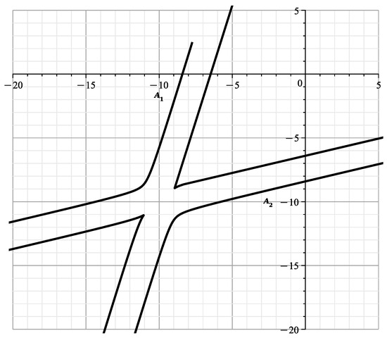
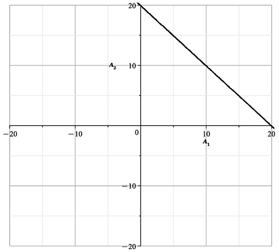
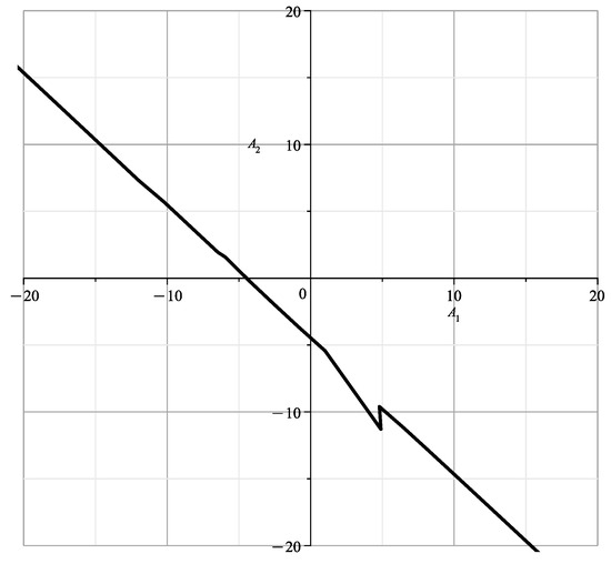
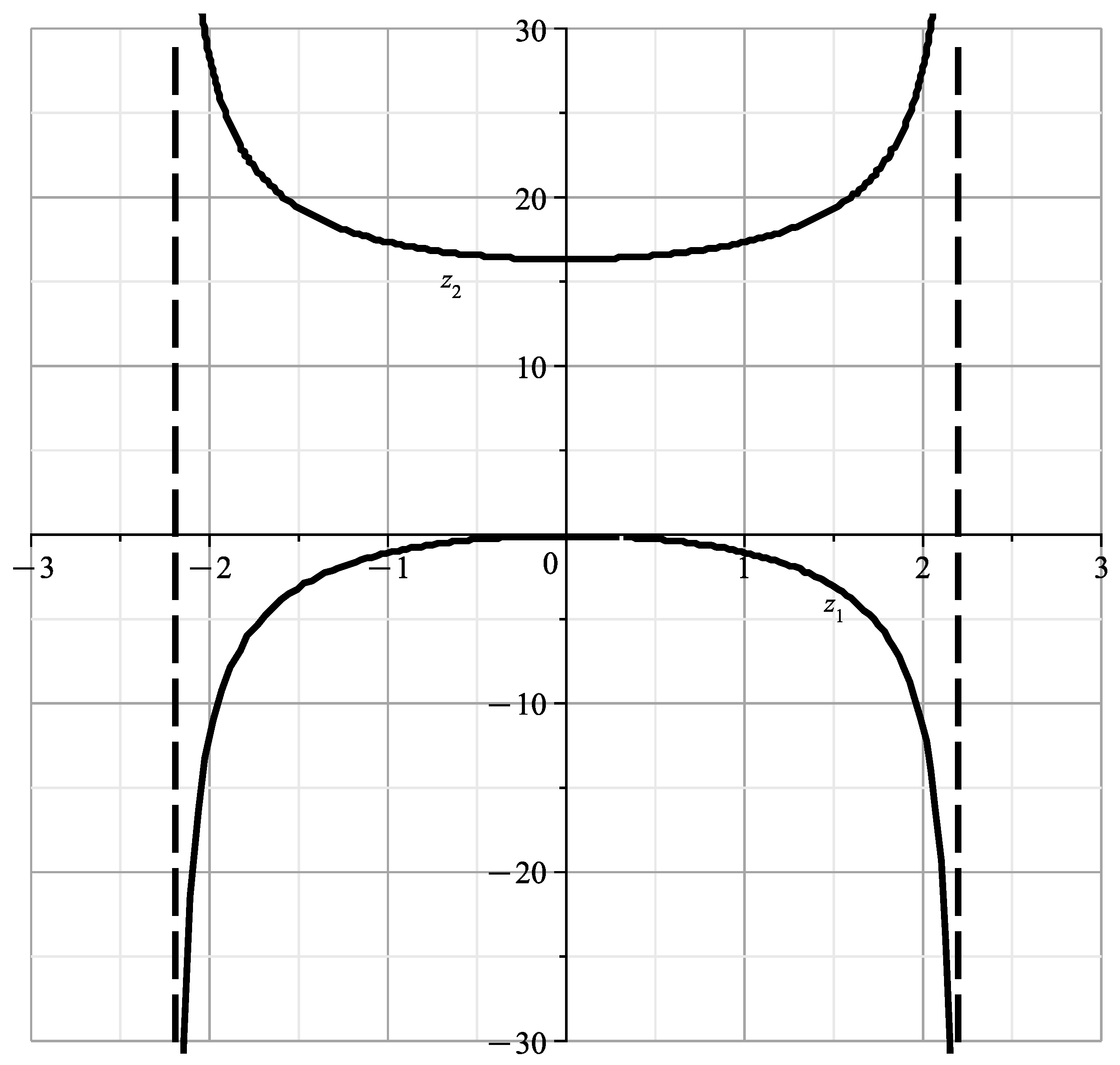
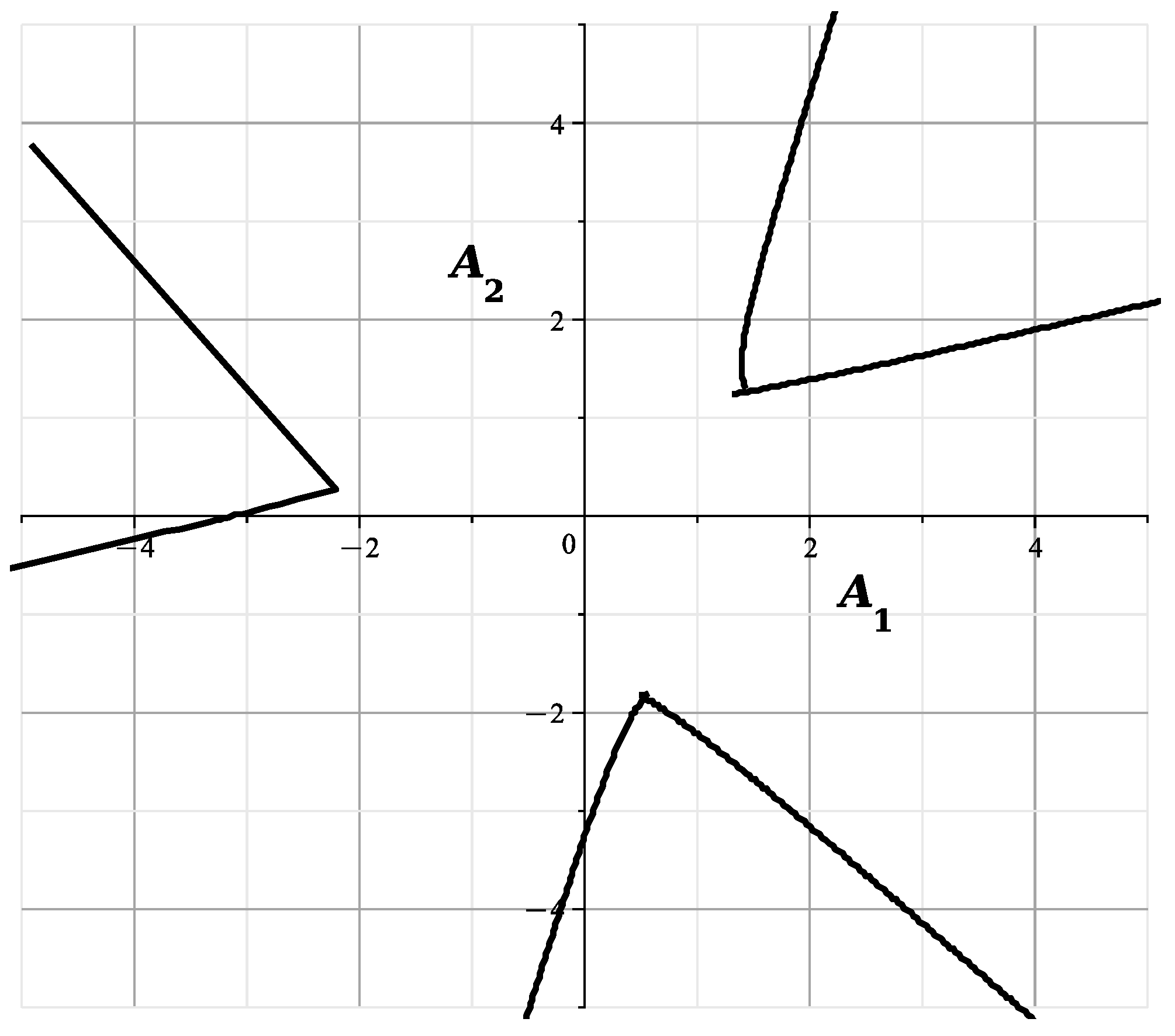
When parameterized by (24), this curve is shown in Figure 7. It is similar to the part of [23] (Figure 12) corresponding to , with parts of branches and .

Figure 7.
Curve (27).
If then and
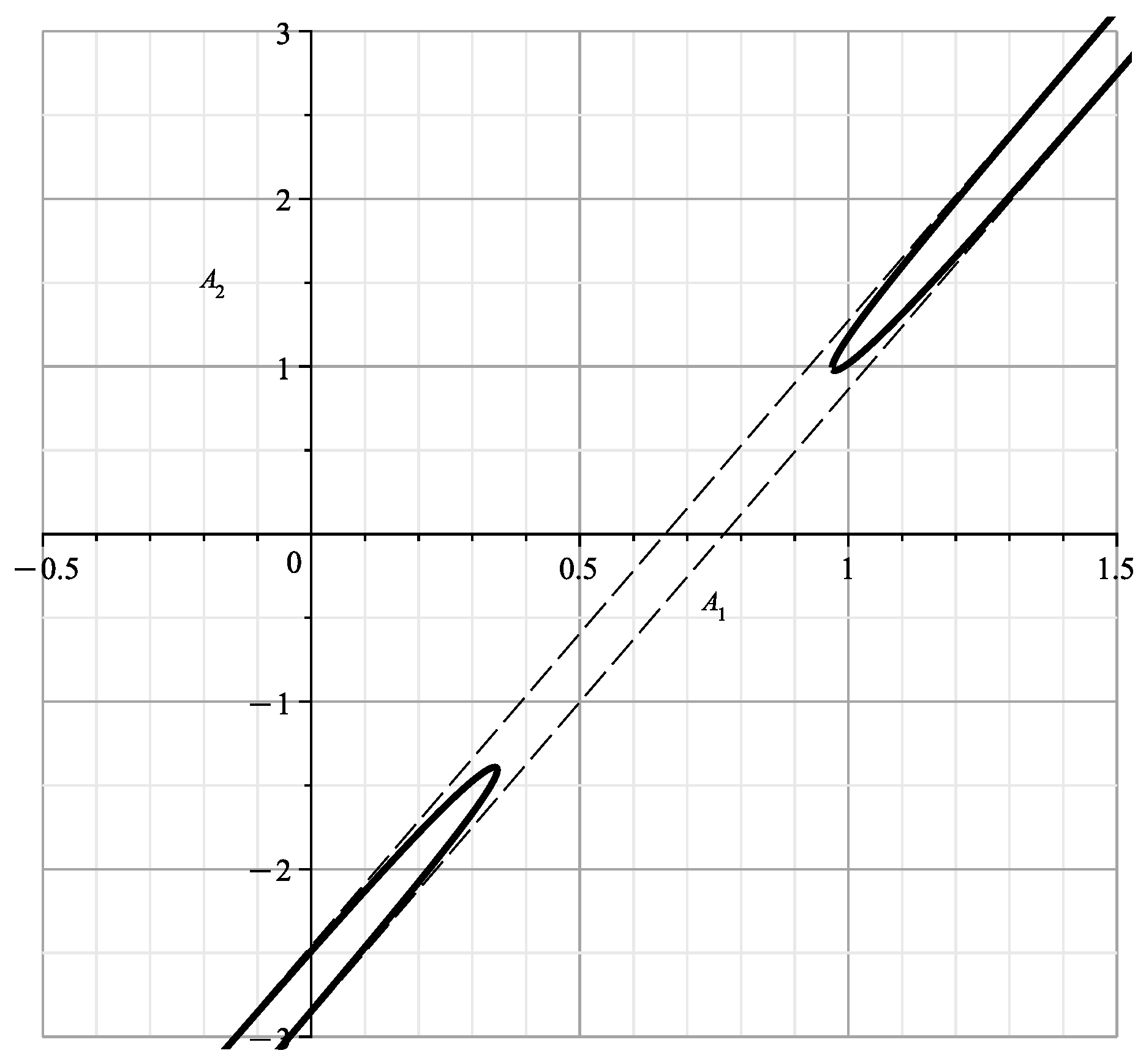
When parameterized by (24), this curve is shown in Figure 8. According to (23) in this figure, when and , 2 branches each merge into one line. These results are similar to those of Section 9 of [1], differing from them by the angle rotation.
Figure 8 is similar to the part of Figure 15 in [23] corresponding to with parts of branches and .

Figure 8.
Curve (28).
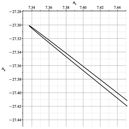
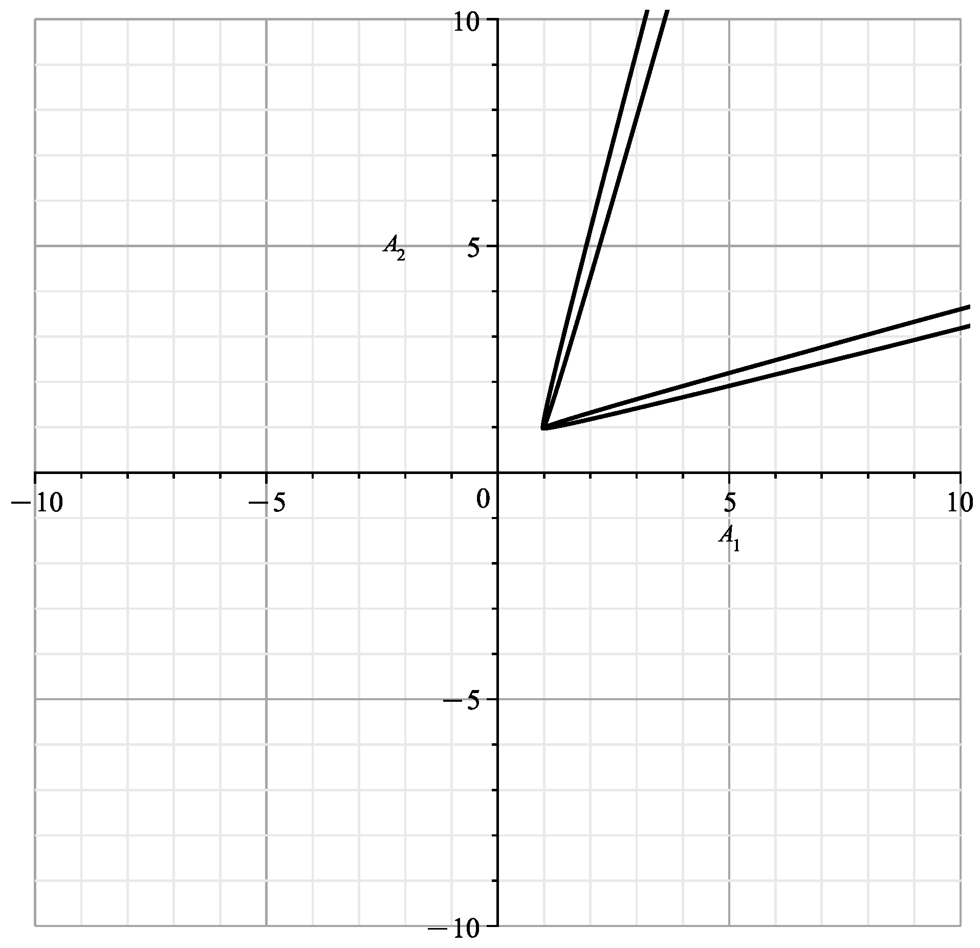
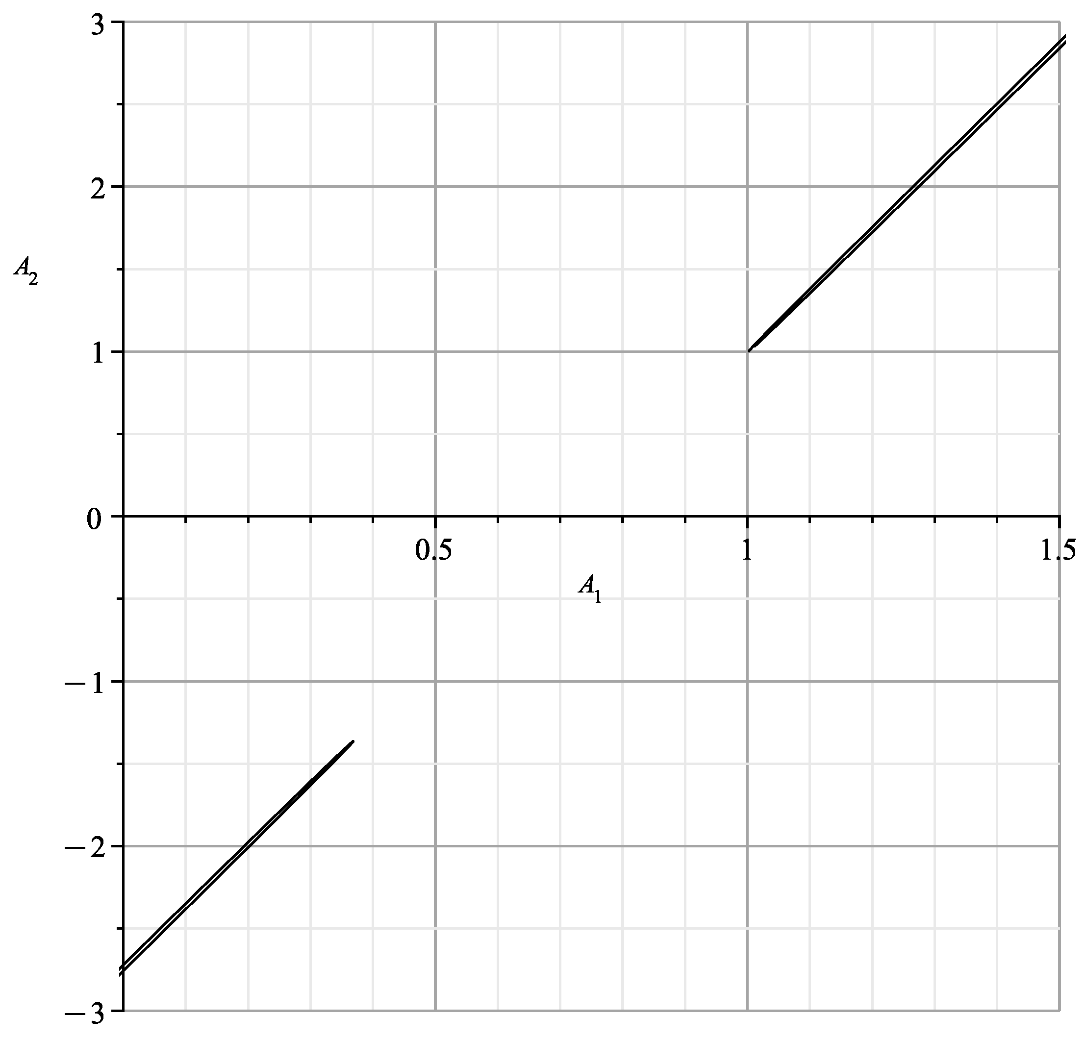
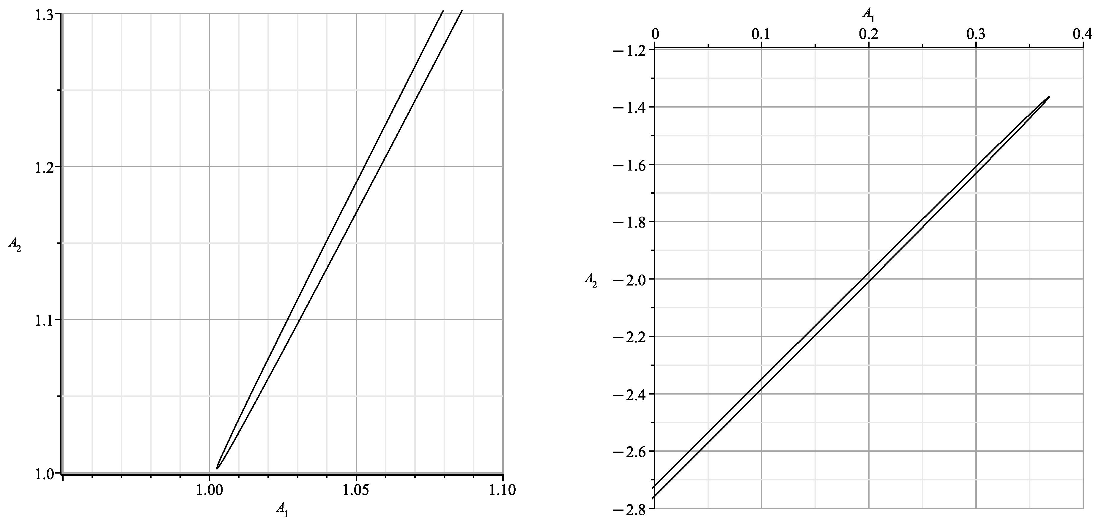
Here the branches are very close and a different scale is needed. We can draw each branch separately, as in Figure 9.
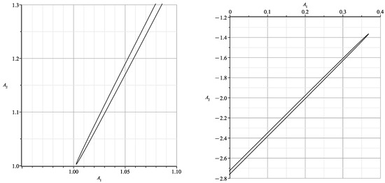
Figure 9.
Curve (28) in more detail.
In that case also there exists a parametric expansions. In the polynomial we make the power transformation (21) and obtain
Here from (22). According to (24) we substitute (17) into polynomials . We obtain with coefficients depending on t via and . We apply Theorem 1 in [1] to the equation and obtain the expansion
So according to (25)
2.5. The Normal
It corresponds to a truncated polynomial
Let’s denote
According to [11], we compute the matrix such that . Since , then we do a power transformation.
and we get
Let us denote
According to (22) the polynomial is obtained from the polynomial by the transposition
So here everything is similar to Section 2.4, but in the plane , rotated by an angle of . Also here there are expansions symmetric to (29) by transpositions (30) and
- Result of Section 2
Theorem 1.
Near the singular point the variety Ω has 3 local singular parametric expansions (18) and (29) and symmetric to (29) by transpositions (30) and (31). The expansions (18) describe parts of branches and very near the point . Expansions (29) and its symmetric describes branches and near line (26) and symmetry line to it. For branches and coincide at parts of these lines.
3. The Structure of the Manifold near the Curve of Singular Points
Recall that the curve is given by equations
In the polynomial , substitute
and write the result as
The polynomials , , , and are computed using the command coeff(R, mu, k) [27]. After factorization, the polynomials , , and have the form:
Let’s denote
Then is divided by , is divided by , and and are not divided by . The curve has genus 0, its parameterization is
and is shown in Figure 10.

Figure 10.
Curve .
According to (32) we substitute
into the polynomials . Then the polynomial (33) will become a polynomial
whereby
where , according to (32). In particular, we obtain
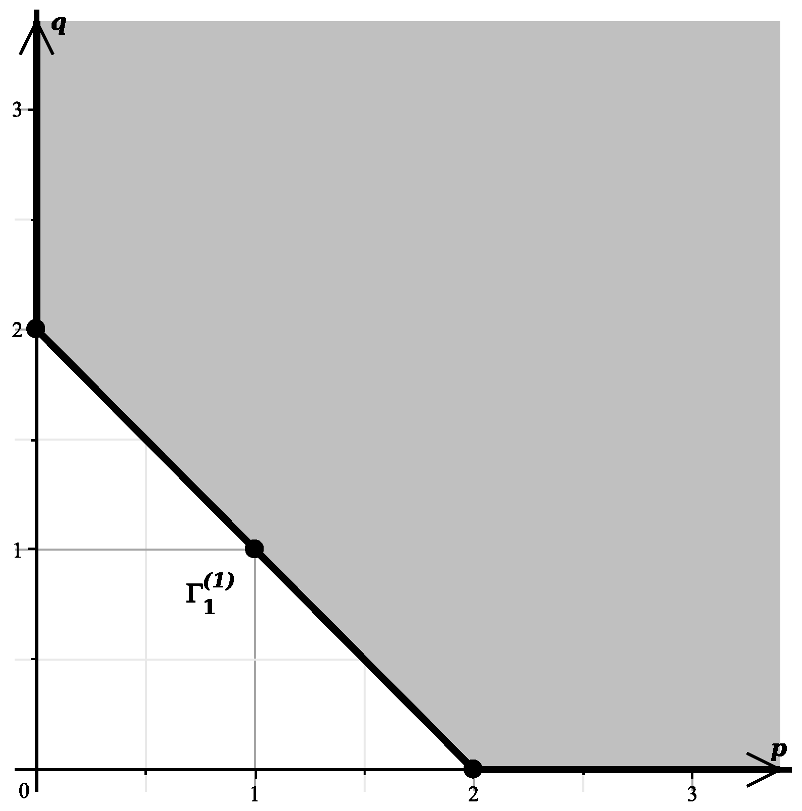
From the Formulas (37) and (38), we can see that the Newton’s polygon of the polynomial (36) in the plane has an edge containing the points , , (Figure 11) with external normal .

Figure 11.
The lower left side of the polygon .
So we’re doing a power transformation
Then the polynomial becomes a polynomial.
where
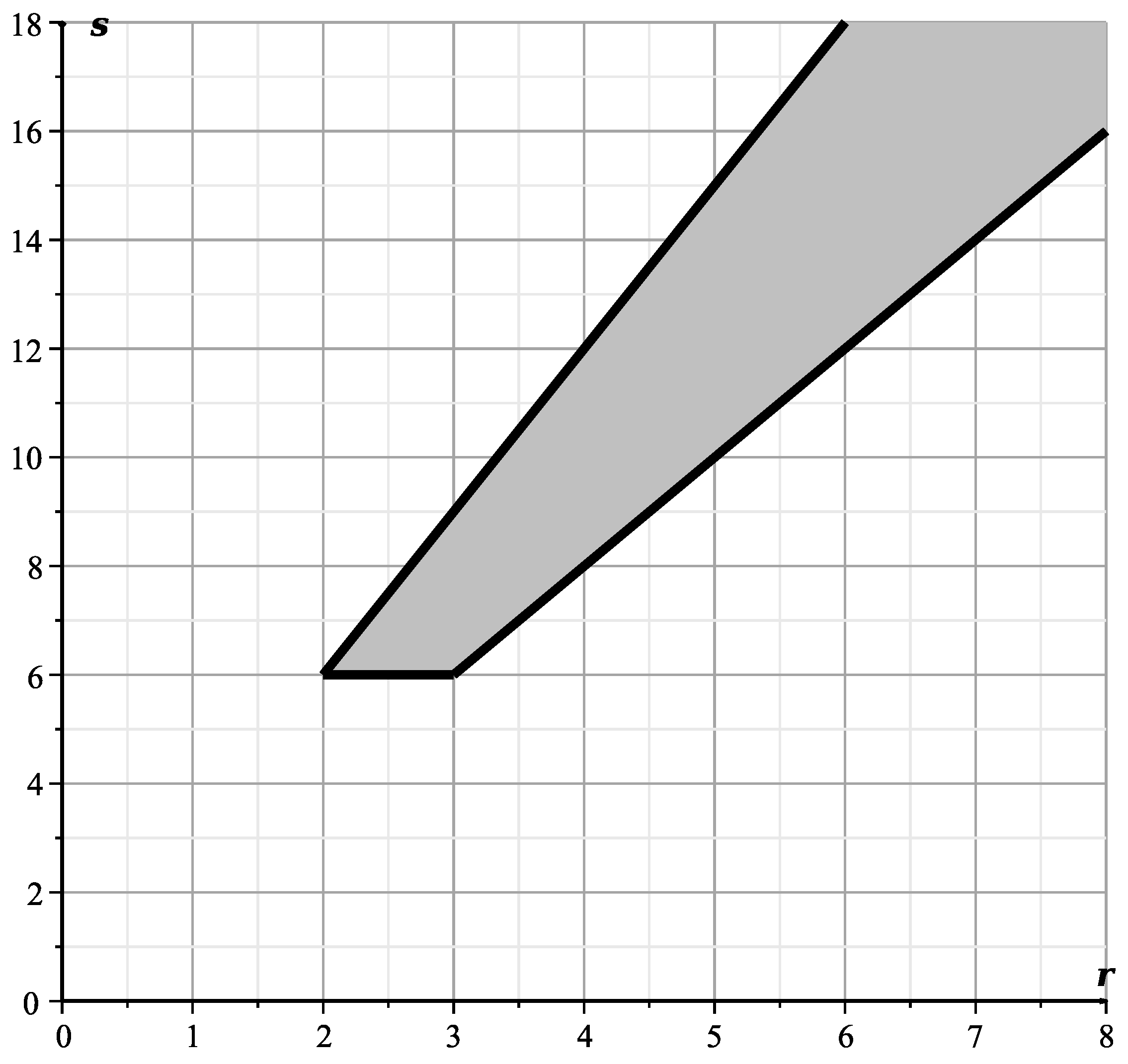
The support and Newton’s polygon for the polynomial are shown in Figure 12.

Figure 12.
The support and polygon of the polynomial .
The truncated equation corresponding to the edge is
It has two roots
Their denominator goes to zero at two real points
These points are indicated in Figure 10.
Next, we consider the expansions of the manifold for the cases of two roots (42).
In the polynomial of (40), we make the substitutions
where are given by the formula (42). We get
where integers . In this case.
where are binomial coefficients. In particular, according to (38), (41) and (42), we have
More specifically,
i.e., . Hence Theorem 1 in [1] is applicable, which for solutions of equations according to (45) and (46) gives the expansions
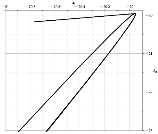
With fixed, the Formulas (47) and (49) are defined in the plane with the first curve , and the Formulas (48) and (49) define there the second curve . We obtain four curves. Restricting ourselves to the initial terms of the expansions, we draw them. When , the curve is
and it is shown in Figure 13.
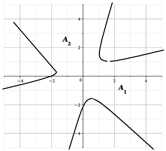
Figure 13.
The curve at .
The curve is
It’s shown in Figure 14.
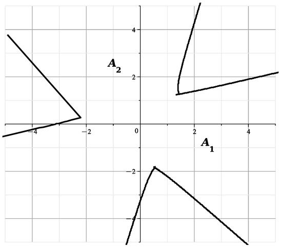
Figure 14.
The curve at .
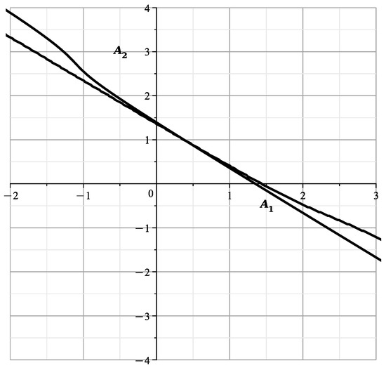
When , the curve
is shown in Figure 15.
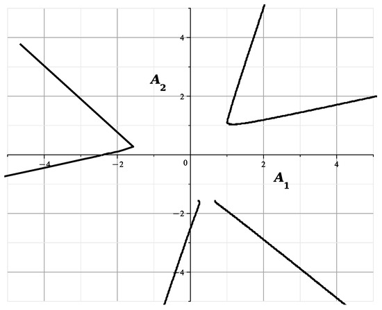
 and the curve
is shown in Figure 16.
and the curve
is shown in Figure 16.
Figure 15.
The curve at .
Figure 15.
The curve at .
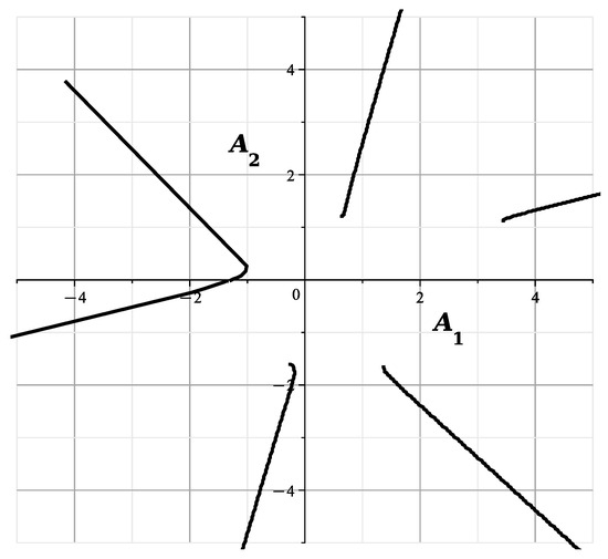
Figure 16.
The curve at .
The curves of Figure 13 and Figure 14 correspond to and are similar to the curves of Figure 13 of [23], showing the section of the variety by the plane . The curves of Figure 15 and Figure 16 correspond to and they are similar to the curves of Figure 14 of [23], showing the cross section of by the plane This confirms the correctness of the calculated expansions.
In Figure 13, Figure 15 and Figure 16, there are discontinuities in the curves at the places of the roots (43) of the denominators and in (42). They can be eliminated by substituting
instead of substitution (35) and calculate the corresponding expansion.
- Result of Section 3
4. The Structure of the Variety near the Curve of Singular Points
We take the polynomial , where , , are elementary symmetric polynomials, and we substitute . Then the polynomial takes the form
Let’s write the polynomial in coordinates, substituting
with .
Then we get a polynomial . We put
The curve consists of singular points, has genus 0, and parameterization
The curve is shown in Figure 17.
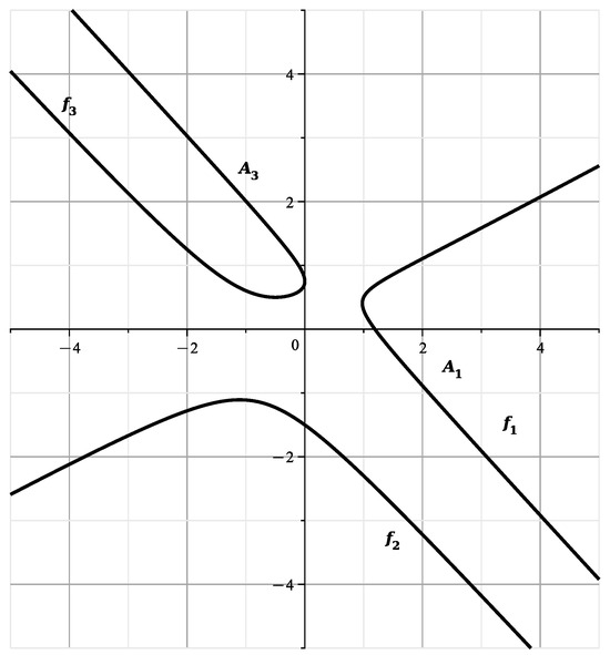
Figure 17.
The curve .
In [23] (Figure 3), the components , , of this curve are shown in gray. The scales on the axes are different there. In the polynomial we substitute
and we get a polynomial depending on three variables,
We factorize for because they are need for our computation and get
and
Then
The multiplier enters in in the third degree, in in the second degree, in , and in it does not enter. Then is divisible by , is divisible by , and and are not divisible by . The curve has genus 0, parameterization (50).
The curve goes to infinity at
Into the polynomials we substitute
according to (50). Then the polynomial (52) will become a polynomial
where , according to (50). In particular, we obtain
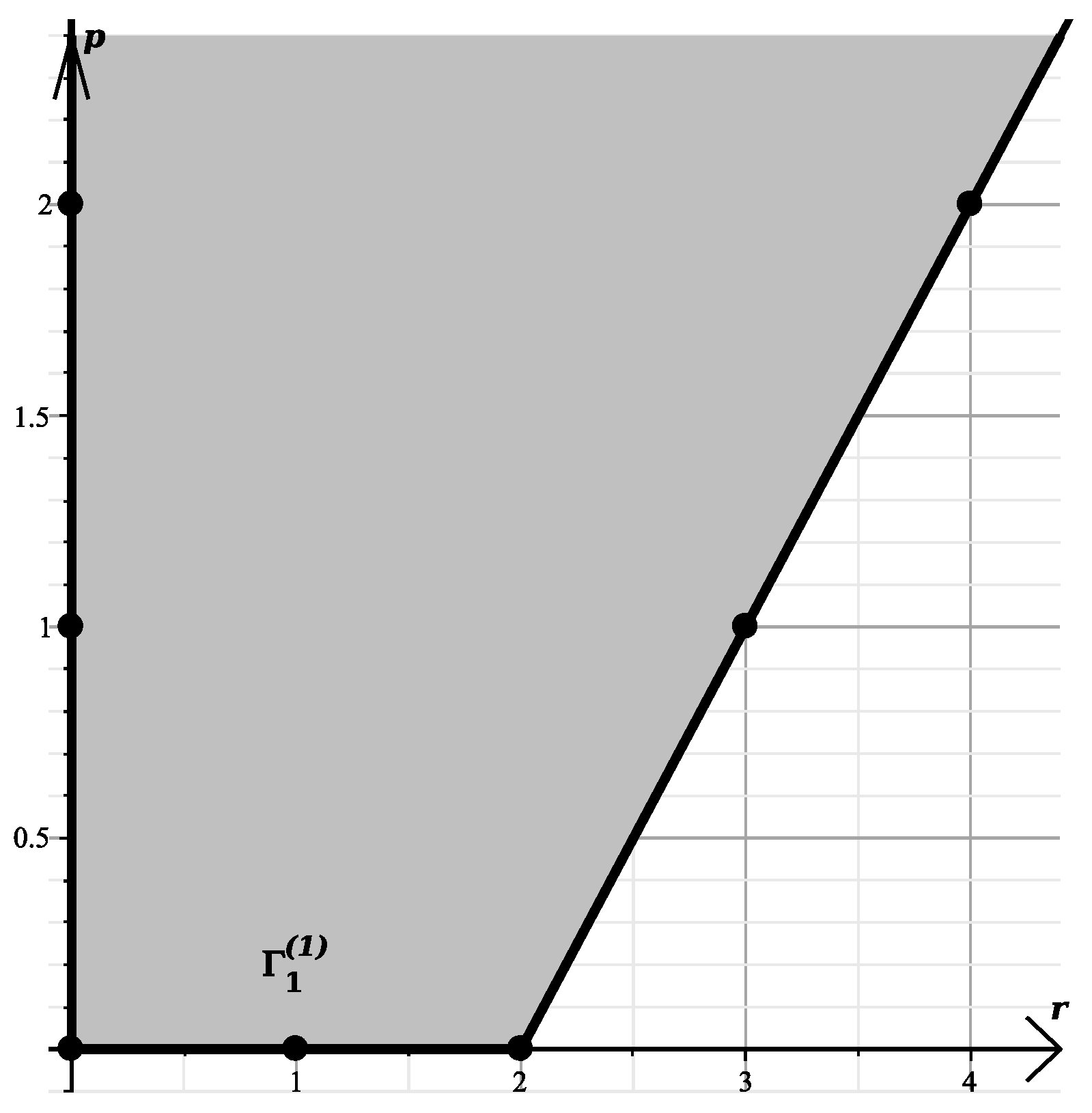
From the Formulas (55) and (57), we can see that the Newton’s polygon of the polynomial given by (54) in the plane has an edge , containing the points , (Figure 18) with external normal .

Figure 18.
Bottom left of the polygon .
A truncated polynomial corresponds to this edge
According to [11] we find the unimodular matrix for such that . Therefore, we need to do a power transformation
where and D are new variables, i.e.,
Since , then . Hence we can write
Then the polynomial becomes a polynomial
where . Thus the polygon of Figure 18 takes the form shown in Figure 19. For the polynomial the polygon is shown in Figure 20. The truncated Equation (57) takes the form of
Figure 19.
The Newton’s polygon of the polynomial .
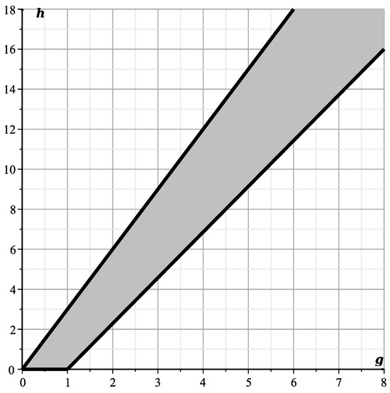
Figure 20.
Newton’s polygon of the polynomial
From where
The only real root of the denominator is
In this case.
After substitution , into the polynomial , we obtain
When , the polynomial is calculated using the command [27]. The quotient at D of degree zero is zero. The coefficient on the first degree of D is obtained by
Therefore, Theorem 1 in [1] is applied to equation , and according to it a solution is
When we get the truncated equation , then it follows
Now let’s go back and get an approximation
The curves (62) and (63) at are shown in Figure 21 and Figure 22, respectively. The gaps in these curves are the neighborhoods of the point of (58). They can be filled in if instead of substituting (51) we do

The closeness of these curves to the curve of Figure 17 confirms the correctness of the found parametric expansion of the (59) of the variety near the curve of singular points.
- Result of Section 4
5. The Variety at Infinity
The number of branches of the variety at infinity exceeds their number near its singularities. Their complete study would exceed 7 sections on branches in the finite domain (4 Section in [1] and 3 Section here). Therefore, we study here only those branches corresponding to the first nonlinear polynomial multiplier included in the truncated polynomial in degree one.
5.1. Reducing the Study at Infinity to the Study in the Finite Domain
In the polynomial , we do a power transformation
The resulting polynomial is divided by and factorized, we get
In the sum , which is not a polynomial, we substitute
The resulting polynomial is . Let us explain the meaning of these transformations for the two-dimensional case, restricting ourselves to coordinates and . The polyhedron of the original polynomial has the form shown in Figure 23.

Figure 23.
Projection of the polyhedron of the polynomial onto the plane .

Figure 24.
Projection of the polyhedron of the polynomial in coordinates .
The polyhedron of sum is shown in Figure 25.

Figure 25.
Projection of the polyhedron of sum .
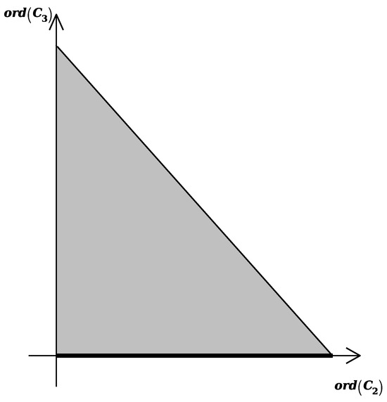
Figure 26.
Projection of the polyhedron of the polynomial .
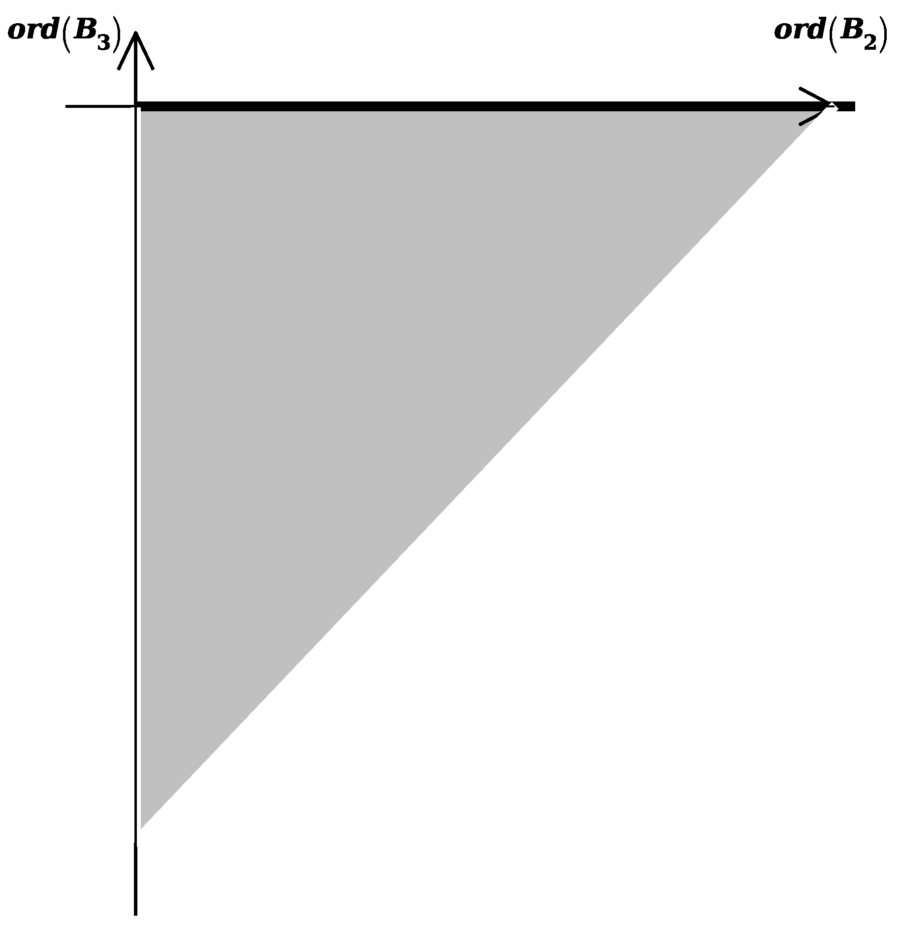
In Figure 23, Figure 24, Figure 25 and Figure 26, the edge that corresponds to infinity in coordinates is bolded.
Now we need to study the polynomial at . For this purpose, we compute the Newton’s polyhedron of the polynomial . Its graph is shown in Figure 27.
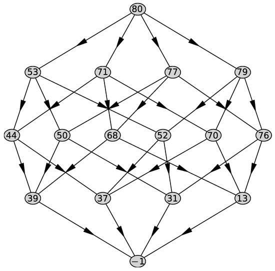
Figure 27.
Graph of polyhedron .
It has 4 two-dimensional faces with external normals
Since and , and , we select the only normal , which has only the third coordinate negative. After factorization, the corresponding truncated polynomial has the form:
We will devote a separate subsection to each of its multipliers.
5.2. The First Multiplier in (66)
Multiplier
does not factorize in the field of rational numbers, but does factorize in the extension of that field with . It is the product of two linear forms , and we will consider the whole thing as a coordinate substitution, where
and put . Its inverse substitution is
We substitute it into the polynomial and get the polynomial . For the polynomial , we compute its Newton’s polyhedron .
Its graph is shown in Figure 28. It has 11 two-dimensional faces with external normals
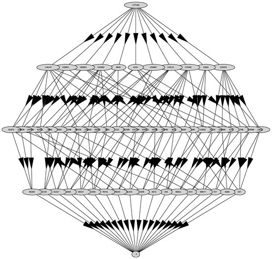
Figure 28.
Graph of polyhedron .
Since and , we select the only normal that has all coordinates negative. This is . It corresponds to the truncated polynomial
After the power transformation
we get , where
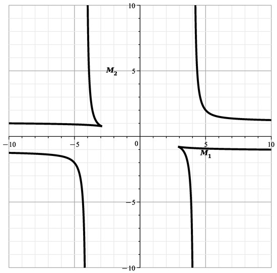
Figure 29.
Curve .
In (70), the denominator has 2 real roots
In (70), the denominator has 2 real roots
In fact, the parametric expansion of the variety can also be calculated here. To do this, we perform a power transformation (68) to the polynomial and similarly to (16) get the polynomial
where . We substitute into the polynomials according to (69) and (70)
We obtain the polynomial with coefficients depending on t via and . In this polynomial.
where
when , , , ,
Specifically
Here the sign means new notation.
Indeed functions and have very complicated forms. So we omit them and give only some their properties.
The function has two multiple roots
of multiplicity 6, and the function has the same roots of multiplicity 8. The denominators of the functions and each have four multiple roots of (71) and (72). By the implicit function theorem [1] (Theorem 1), the equation has a solution as a power series on
where are the rational functions of t, which are expressed through the coefficients which in turn are expressed through and according to (74). This expansion is valid for all values of except maybe the neighborhood of the roots of (75). In particular,
where the denominator has no real roots. According to (76) approximately.
By the sequence of substitutions (64), (65), (67), (68) and (73), we return to the original coordinates, which at small by are approximated with
According to (65)
5.3. Second Multiplier in (66)
Polynomial
does not factorize in the field of rational numbers, but does factorize in the extension of that field with . It is the product of two linear forms , which we treat as coordinate substitutions
Its inverse substitution is
We substitute it into the polynomial and get the polynomial For the polynomial , we calculate Newton’s polyhedron .
Its graph is shown in Figure 32. It has 11 two-dimensional faces with external normals
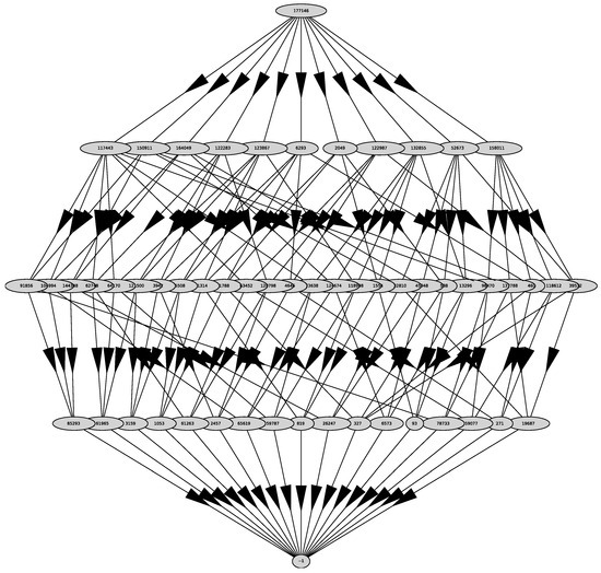
Figure 32.
Graph of Polyhedron .
Since and , we select the only normal that has all coordinates negative. This is the normal . It corresponds to the truncated polynomial
Assume
The inverse transformation is
We substitute it into the polynomial and get the polynomial . For the polynomial , we compute Newton’s polyhedron .
Its graph is shown in Figure 33. It has 9 two-dimensional faces with external normals
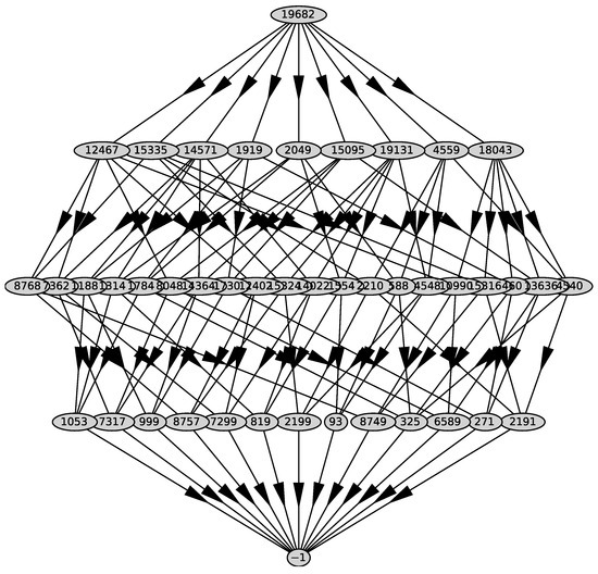
Figure 33.
Graph of polyhedron .
Since , , and , we select the only normal that has all coordinates negative. This is According to results of our program, it corresponds to the truncated polynomial
Doing the power transformation
and factorize we get
If we substitute , into the polynomial in parentheses, it is equal to . Therefore, the power transformation (81) is substituted into the large polynomial and divided by we get the polynomial . We compute its Newton polyhedron .
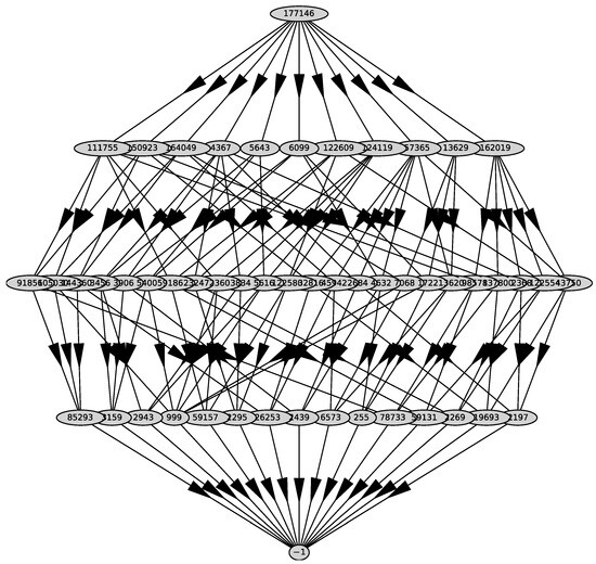
Figure 34.
Graph of polyhedron .
Since , , and , we select the only normal that has all coordinates negative. This is . The corresponding shortening
Doing the power transformation.
and we get
where addition “” indicate that it is after power transformation.
If we substitute inside the brackets, we get the factorization
The power transformation (82) we do in the polynomial , we get the polynomial .
In , we substitute, introducing new variables ,
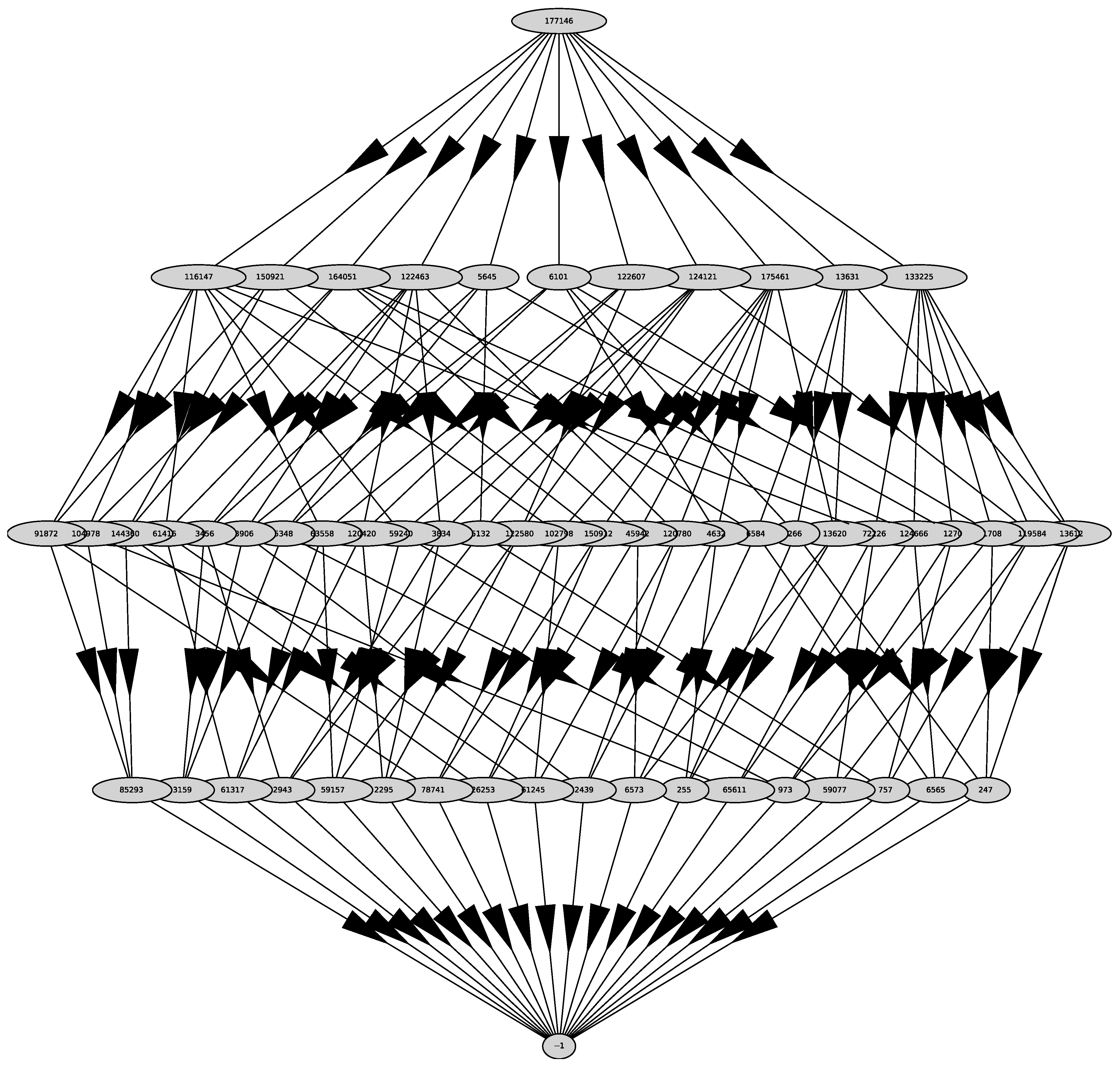
We get the polynomial and for it we calculate Newton’s polyhedron .
Its graph is shown in Figure 35. The computer computed the polyhedron in 87 h and 23 min. It has 9 two-dimensional faces with exterior normals
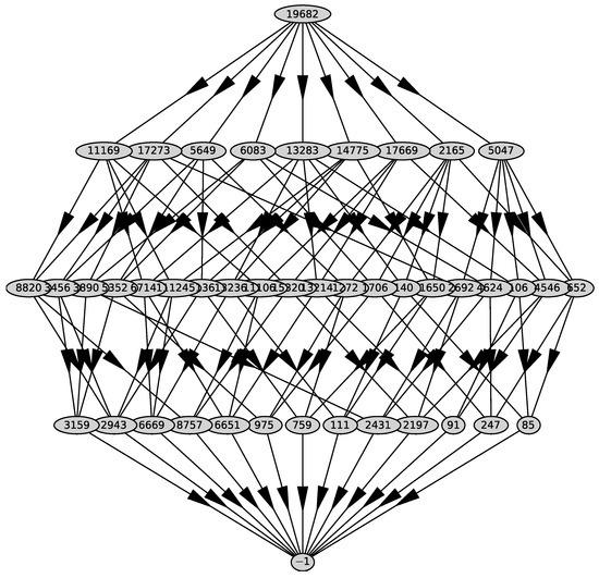
Figure 35.
Graph of polyhedron .
Since , , and , we select the only normal that has all coordinates negative. This is . The corresponding truncation
We do a power transformation.
Then
The curve has genus 0, and parameterization
and is shown in Figure 36.

Figure 36.
Curve .
Figure 36 shows the limiting values of when the branch goes to infinity. The approximate values of the zeros of the numerators in (85) are. for and for .
Into the polynomial we substitute
according to (85). Then the polynomial becomes a polynomial
whereby
where according to (85). In particular, from (86)–(88) we obtain
According to [1] (Theorem 1), the solution to the equation has the form, , where
The denominators in and in (85) have root .
Now let’s go back and approximately from (84) obtain
Substitute that into (83).

5.4. Third Multiplier in (66)
It is a linear multiplier defined with
The substitution is
Its inverse substitution is
Let’s consider all of this as a coordinate substitution in the polynomial . We substitute it into the polynomial and get the polynomial . For the polynomial , we compute Newton’s polyhedron
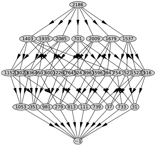
Figure 39.
Graph of polyhedron .
Since , , and , we select the only normal whose first and third coordinates are negative. This is the normal . It corresponds to a truncated polynomial
Do a power transformation.
Then ftr701 after the power transformation (98) is
where . The curve has genus 0, and parameterization
and is shown in the Figure 40.
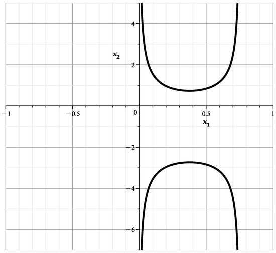
Figure 40.
Curve .
The curve goes to infinity at
Into the polynomial we substitute
according to (99). Then the polynomial becomes a polynomial
whereby
where according to (99). In particular, from (101)–(103) we obtain
According to Theorem 1 of [1], the solution of equation is
, where
The denominator in has roots (100).
Now let’s go back and approximate from (102) obtain
Substitute that into (98) and we get
In Figure 41, Figure 42, Figure 43 and Figure 44, are shown the curves of (106) and (107) for values , , 1, , respectively.

The another branch is symmetric to this one with respect to the line .
5.5. Fourth Multiplier in (66)
5.5.1. Preliminary Calculations
The 4th multiplier is a linear multiplier . Let’s do the substitution , , . Its inverse substitution is
We treat it all as a coordinate transformation in the polynomial . We substitute it into the polynomial and get the polynomial . For the polynomial , we compute Newton’s polyhedron , with graph given in Figure 45. It has 7 two-dimensional faces with external normals
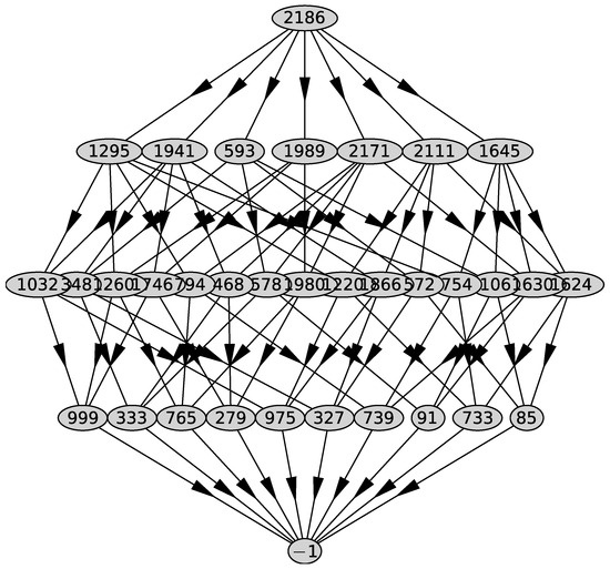
Figure 45.
Graph of Polyhedron .
Since , , and , we select the only normal that has negative first and third coordinates. This is and it corresponds to the truncated polynomial
Let’s do the substitution , , . Its inverse substitution is
and treat it all as a coordinate change in the polynomial . Substitute it into the polynomial and get the polynomial . For the polynomial , we calculate Newton’s polyhedron .
Its graph is shown in Figure 46. It has 8 two-dimensional faces with external normals
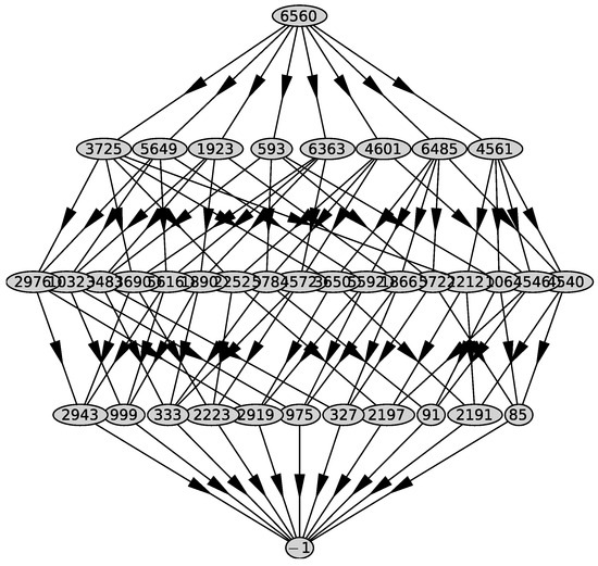
Figure 46.
Graph of polyhedron .
Since , , and , we select two normals whose first and third coordinates are negative. These are and . We will deal with them in separate subsubsections.
5.5.2. The Normal
According to result of our program it corresponds to a truncated polynomial
Making a power transformation
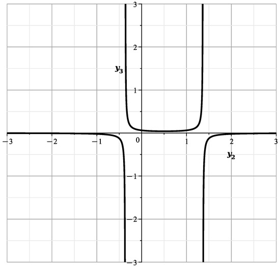
Figure 47.
Curve .
In (112), the denominator in has 2 real roots
In fact, here we can also compute the parametric expansion of the manifold. To do this, we do the power transformation (110) in the polynomial and get the polynomial
In the polynomials according to (112) we substitute
We obtain the polynomial with coefficients depending on t through and . In this polynomial
where when , , , , . Specifically,
The function has real roots
and the function has 2-multiple roots , and
By the Implicit Function Theorem [1] (Theorem 1), the equation has a solution as a power series on
where are rational functions of t, which are expressed through the coefficients , which in turn are expressed through and according to (110). This expansion is valid for all values of except maybe the neighborhood of the roots of (114). In particular,
where the denominator has 2 real roots and of (114). Approximately we get
Let’s return to the previous coordinates, which are approximated to be equal for small on the manifold

5.5.3. The Normal from (110)
It corresponds to a truncated polynomial
By the power transformation
We have
where . The curve has genus 0, and parameterization
It is shown in Figure 50.

Figure 50.
Curve .
In (122), the denominator in has 2 real roots given by (113). In fact, the parametric expansion of the manifold can also be calculated here. To do this, we do a power transformation (121) in the polynomial and get the polynomial
Into the polynomials we substitute
according to (122).
We obtain the polynomial with coefficients depending on t through and In this polynomial
where where , , , . Specifically
The function has real roots (114). By the Implicit Function Theorem [1] (Theorem 1), the equation has a solution as a power series on
where are rational functions of t, which are expressed through the coefficients , which in turn are expressed through and according to (122). This expansion is valid for all values of except maybe the neighborhood of the roots of the polynomial (123). In particular,
where the denominator has 2 real roots and of (114). We get an approximation
Let’s return to the previous coordinates, which, for small on , are approximately equal to
6. Conclusions
In the paper we show that all parametric expansions of variety near its singularities and infinity can be computed with any accuracy and compute their first terms. We consider a very rich set of cases and find the ways to finish computations in all of them.
We do not intend to explain our results for original problems of Ricci flows and Einstein’s metrics. Let it will be done by authors of [14,15,16,17,18,19,20,21,22], who are specialists in the problem.
Author Contributions
Conceptualization, A.D.B.; methodology, A.D.B.; software, A.A.A.; validation, A.D.B.; writing—original draft preparation, A.A.A.; writing—review and editing, A.D.B.; visualization, A.A.A. All authors have read and agreed to the published version of the manuscript.
Funding
This research received no external funding.
Data Availability Statement
Data are contained within the article.
Acknowledgments
The authors are grateful to A.B. Batkhin for his help in the software implementation of algorithms and manuscript preparation.
Conflicts of Interest
The authors declare no conflict of interest.
References
- Bruno, A.D.; Azimov, A.A. Parametric Expansions of an Algebraic Variety near Its Singularities. Axioms 2023, 5, 469. [Google Scholar] [CrossRef]
- Newton, I. A treatise of the method of fluxions and infinite series, with its application to the geometry of curve lines. In The Mathematical Works of Isaac Newton; Woolf, H., Ed.; Johnson Reprint Corp.: New York, NY, USA; London, UK, 1964; Volume 1, pp. 27–137. [Google Scholar]
- Puiseux, V. Recherches sur les fonctions algebriques. J. Math. Pures et Appl. 1850, 15, 365–480. [Google Scholar]
- Chebotarev, N. The “Newton polygon” and its role in current developments in mathematics. In Isaak Newton; Izdatel’stvo Akademii Nauk SSSR: Moscow, Russia, 1943; pp. 99–126. (In Russian) [Google Scholar]
- Abhyankar, S.S.; Moh, T. Newton-Puiseux expansion and generalized Tschirnhausen transformation. I. J. Reine Angew. Math. 1973, 260, 47–83. [Google Scholar] [CrossRef]
- Abhyankar, S.S.; Moh, T. Newton-Puiseux expansion and generalized Tschirnhausen transformation. II. J. Reine Angew. Math. 1973, 261, 29–54. [Google Scholar] [CrossRef]
- Sathaye, A. Generalized Newton-Puiseux expansion and Abhyankar-Moh semigroup theorem. Invent. Math. 1983, 74, 149–157. [Google Scholar] [CrossRef]
- Hironaka, H. Resolution of singularities of an algebraic variety over a field of characteristic zero: I. Ann. Math. 1964, 79, 109–203. [Google Scholar] [CrossRef]
- Hironaka, H. Resolution of singularities of an algebraic variety over a field of characteristic zero: II. Ann. Math. 1964, 79, 205–326. [Google Scholar] [CrossRef]
- Kollár, J. Lectures on Resolution of Singularities; Annals of Mathematic Studies; Princeton University Press: Princeton, NJ, USA, 2007. [Google Scholar]
- Bruno, A.D.; Azimov, A.A. Computation of unimodular matrices of power transformations. Program. Comput. Softw. 2023, 49, 32–41. [Google Scholar] [CrossRef]
- Bruno, A. Nonlinear Analysis as a Calculs. Lond. J. Res. Sci. Nat. Form. 2023, 23, 1–31. [Google Scholar]
- Bruno, A.D.; Batkhin, A.B. Asymptotic forms of solutions to system of nonlinear partial differential equations. Universe 2023, 9, 35. [Google Scholar] [CrossRef]
- Besse, A.L. Einstein Manifolds; Springer: Berlin, Germany, 1987. [Google Scholar]
- Abiev, N.A.; Arvanitoyeorgos, A.; Nikonorov, Y.G.; Siasos, P. The dynamics of the Ricci flow on generalized Wallach spaces. Differ. Geom. Its Appl. 2014, 35, 26–43. [Google Scholar] [CrossRef]
- Abiev, N.A.; Arvanitoyeorgos, A.; Nikonorov, Y.G.; Siasos, P. The Ricci flow on some generalized Wallach spaces. In Geometry and Its Applications; Springer Proceedings in Mathematics & Statistics; Rovenski, V., Walczak, P., Eds.; Springer: Berlin/Heidelberg, Germany, 2014; Volume 72, pp. 3–37. [Google Scholar]
- Abiev, N.A.; Arvanitoyeorgos, A.; Nikonorov, Y.G.; Siasos, P. The normalized Ricci flow on generalized Wallach spaces. In Mathematical Forum; Studies in Mathematical Analysis; Yuzhnii Matematicheskii Institut, Vladikavkazskii Nauchnii Tsentr Rossiyskoy Akademii Nauk: Vladikavkaz, Russia, 2014; Volume 8, pp. 25–42. (In Russian) [Google Scholar]
- Chen, Z.; Nikonorov, Y.G. Invariant Einstein Metrics on Generalized Wallach Spaces. arXiv 2015, arXiv:1511.02567. [Google Scholar] [CrossRef]
- Abiev, N.A. On topological structure of some sets related to the normalized Ricci flow on generalized Wallach spaces. Vladikavkaz Math. J. 2015, 17, 5–13. [Google Scholar]
- Abiev, N.A.; Nikonorov, Y.G. The evolution of positively curved invariant Riemannian metrics on the Wallach spaces under the Ricci flow. Ann. Glob. Anal. Geom. 2016, 50, 65–84. [Google Scholar] [CrossRef]
- Nikonorov, Y.G. Correction to: Classification of generalized Wallach spaces. Geom. Dedicata 2021, 214, 849–851. [Google Scholar] [CrossRef]
- Jablonski, M. Homogeneous Einstein manifolds. Rev. Unión Matemática Argent. 2023, 64, 461–485. [Google Scholar] [CrossRef]
- Bruno, A.D.; Batkhin, A.B. Investigation of a real algebraic surface. Program. Comput. Softw. 2015, 41, 74–82. [Google Scholar]
- Batkhin, A.B. A real variety with boundary and its global parameterization. Program. Comput. Softw. 2017, 43, 75–83. [Google Scholar] [CrossRef]
- Batkhin, A.B. Parameterization of the Discriminant Set of a Polynomial. Program. Comput. Softw. 2016, 42, 65–76. [Google Scholar] [CrossRef]
- Sendra, J.R.; Sevilla, D. First steps towards radical parametrization of algebraic surfaces. Comput. Aided Geom. Des. 2013, 30, 374–388. [Google Scholar] [CrossRef]
- Thompson, I. Understanding Maple; Cambridge University Press: Cambridge, UK, 2016. [Google Scholar]


Disclaimer/Publisher’s Note: The statements, opinions and data contained in all publications are solely those of the individual author(s) and contributor(s) and not of MDPI and/or the editor(s). MDPI and/or the editor(s) disclaim responsibility for any injury to people or property resulting from any ideas, methods, instructions or products referred to in the content. |
© 2024 by the authors. Licensee MDPI, Basel, Switzerland. This article is an open access article distributed under the terms and conditions of the Creative Commons Attribution (CC BY) license (https://creativecommons.org/licenses/by/4.0/).