
On Non-Linear Differential Systems with Mixed Boundary Conditions

Abstract
1. Introduction and Subsidary Statements
2. Parametrization and Convergence of Successive Approximations
- 1.
- The functions of the sequence (27) belonging to the domain are continuosly differentiable on the interval , and satisfy the two-point periodic boundary conditions (25b) and converges uniformly as with respect to the domain to the limit functionwhich satisfies the periodic boundary conditions (25b).
- 2.
- 3.
- The limit functions for all are the unique continuously differentiable solutions of the parametrized integral equationsor, equivalently, of the Cauchy problems for the modified system of integro-differential equations:where and are the mappings given by the formulas
- 4.
3. Connection of the Limit Functions , to the Solution of the Original Problem
4. Solvability Analysis Based on the Approximate Determining System
5. Conclusions
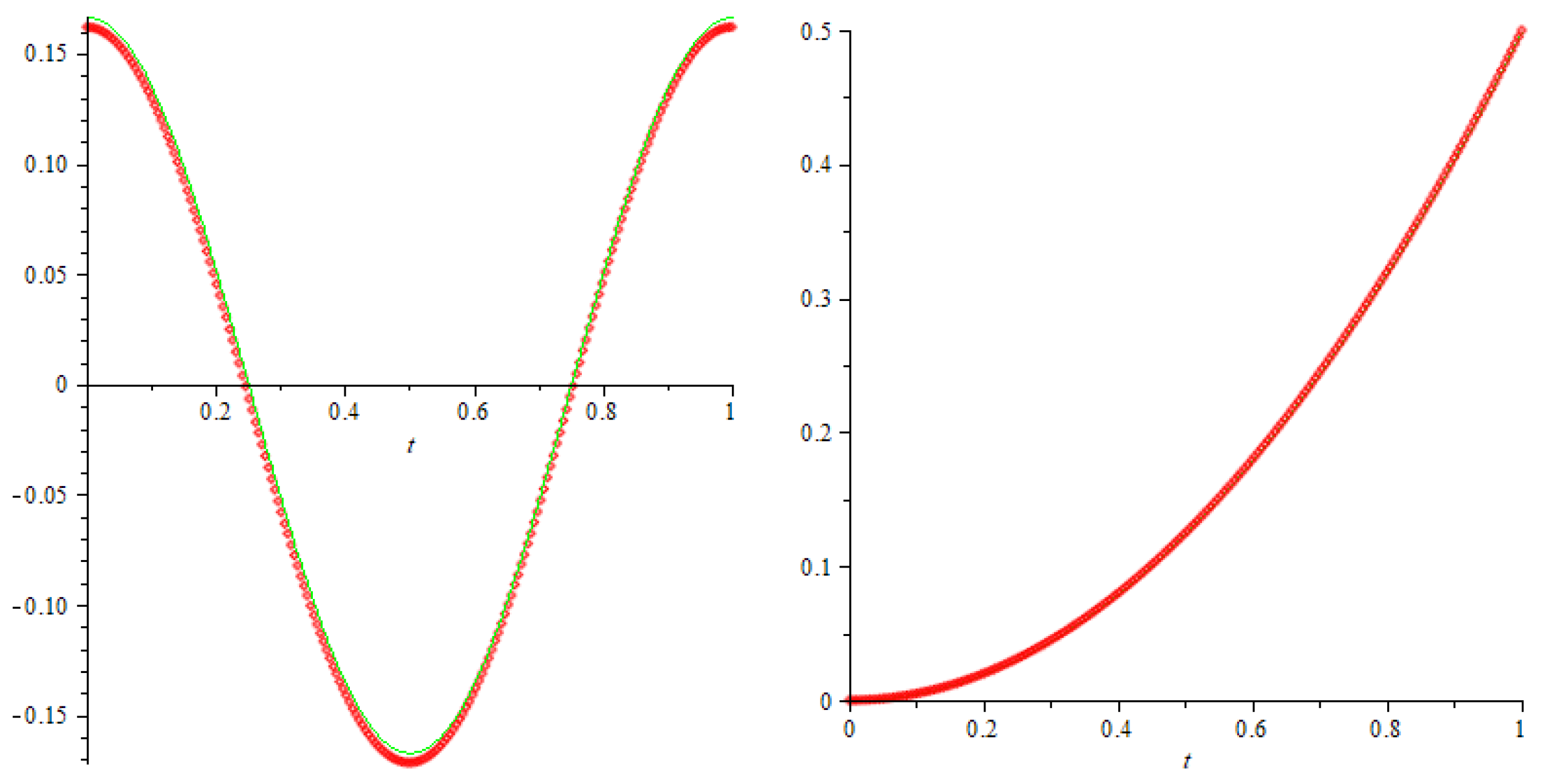
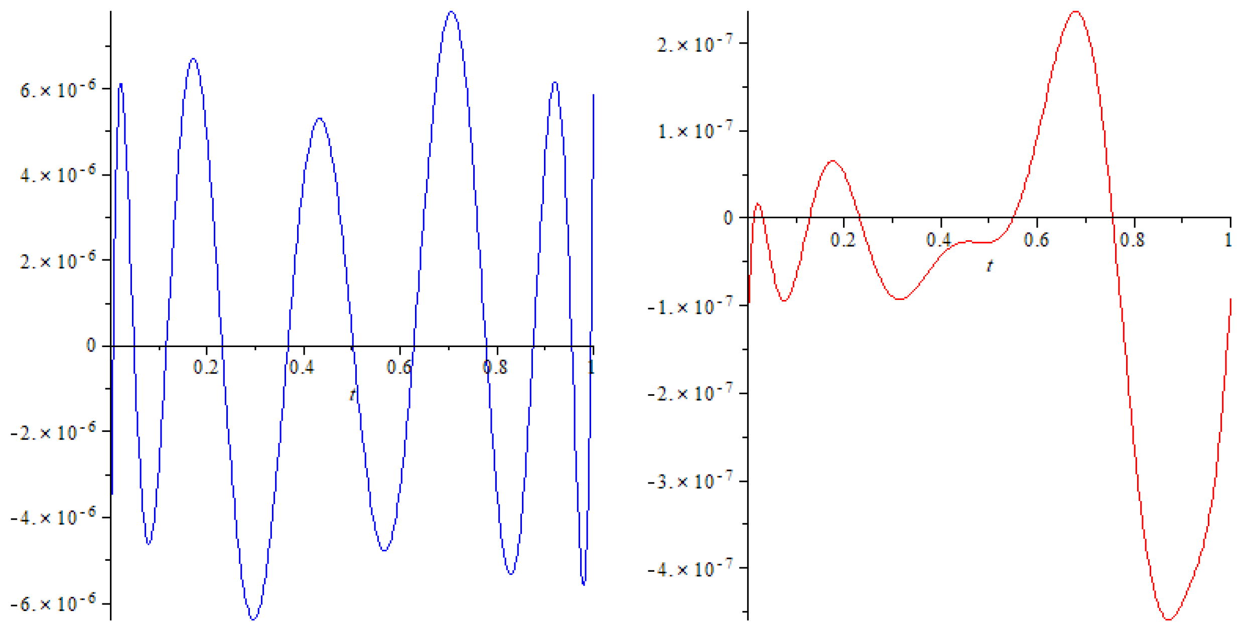
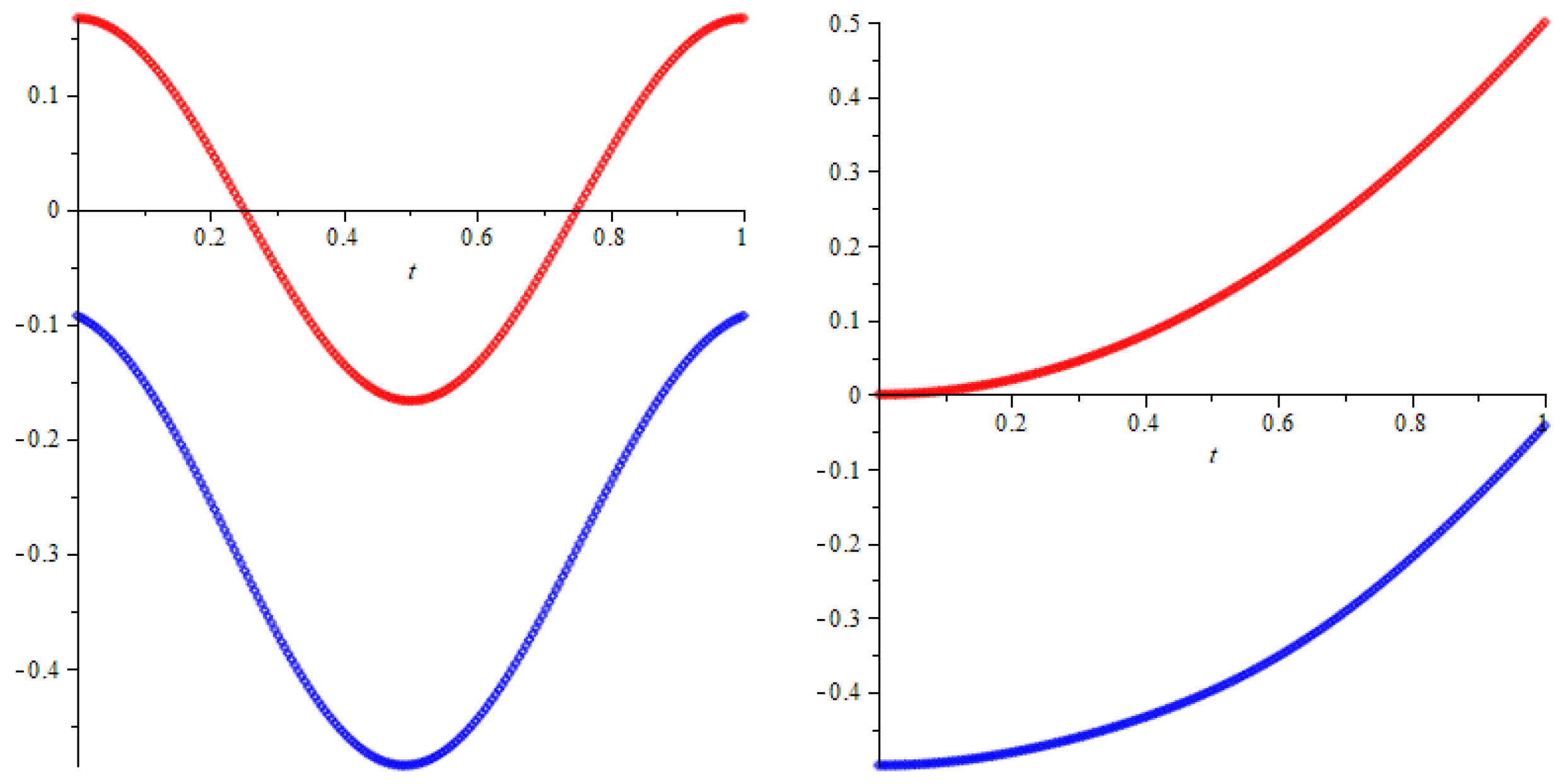
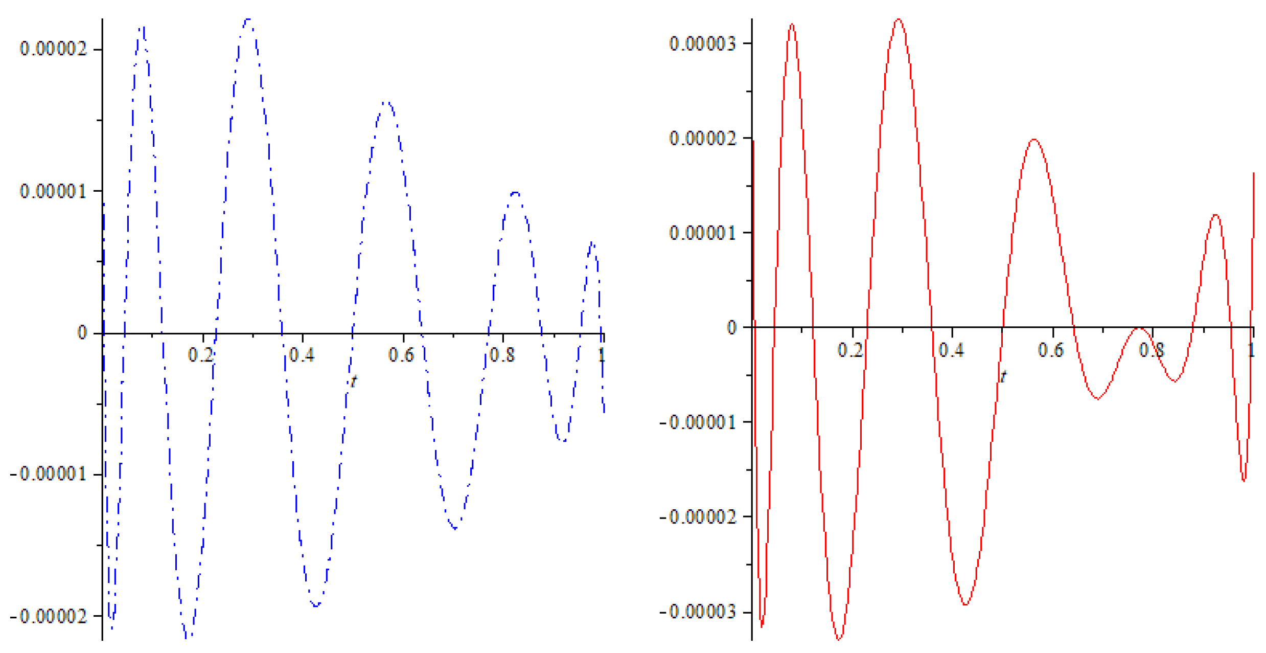
6. Example
6.1. Approximations for the Exact Solution
6.2. Approximations for the Second Solution
Funding
Data Availability Statement
Conflicts of Interest
References
- Samoilenko, A.M. Numerical-analytic method for the investigation of periodic systems of ordinary differential equations. I. Ukr. Math. Zhurnal 1965, 17, 82–93. [Google Scholar]
- Samoilenko, A.M. Numerical-analytic method for the investigation of periodic systems of ordinary differential equations. II. Ukr. Math. Zhurnal 1966, 18, 50–59. [Google Scholar]
- Samoilenko, A.M. On periodic solutions of nonlinear second -order equations. Differ. Uravn. 1967, 3, 1903–1913. [Google Scholar]
- Rontó, A.; Rontóová, N. On constuction of solutions of linear differential systems with argument deviations of mixed type. Symmetry 2019, 12, 1740. [Google Scholar] [CrossRef]
- Samoilenko, A.M.; Laptinsky, V.N. On estimates of periodic solutions of differential equations. Dokl. Akad. Nauk. Ukr. SSR Ser. A 1982, 30–32. (In Russian) [Google Scholar]
- Samoilenko, A.M.; Ronto, V.A. Numerical-analytic method for solving boundary-value problems for ordinary differential equations. Ukr. Math. J. 1981, 33, 356–362. [Google Scholar] [CrossRef]
- Evkhuta, N.A.; Zabreiko, P.P. On the convergence of the Samoilenko method of successive approximations for finding periodic solutions. Dokl. Akad. Nauk. Belarus. SSR 1985, 29, 15–18. (In Russian) [Google Scholar]
- Evkhuta, N.A.; Zabreiko, P.P. On the Samoilenko method for finding periodic solutions of quasilinear differential equations in a Banach space. Ukr. Math. Zhurnal 1985, 37, 162–168. (In Russian) [Google Scholar]
- Evkhuta, N.A.; Zabreiko, P.P. The Poincare method and Samoilenko method for the construction of periodic solutions to ordinary differential equations. Math. Nachrichten 1991, 153, 85–99. [Google Scholar] [CrossRef]
- Pylypenko, V.; Rontó, A. A singular problem for functional differential equations with decreasing non-linearities. Math. Methods Appl. Sci. 2021, 44, 11076–11088. [Google Scholar] [CrossRef]
- Samoilenko, A.M.; Le Lyong, T. A method for studing boundary value problems with nonlinear boundary conditions. Ukr. Math. Zhurnal 1991, 42, 844–850. [Google Scholar] [CrossRef]
- Augustynovicz, A.; Kwapisz, M. On numerical-analytic method of solving of boundary value problems for functional-differential equation of neutral type. Math. Nachrichten 1990, 145, 255–269. [Google Scholar] [CrossRef]
- Kwapisz, M. Some remarks on integral equations arising in applications of the numerical- analytic method for the solution of boundary- value problems. Ukr. Math. Zhurnal 1992, 44, 128–132. [Google Scholar]
- Kwapisz, M. On modification of the integral equation of A.M. Samoilenko’s method. Math. Nachrichten 1992, 157, 125–135. [Google Scholar] [CrossRef]
- Samoilenko, A.M. On a convergence of polynomials and the radius of convergence of its Abel-Poisson sum. Ukr. Math. J. 2003, 55, 1119–1130. [Google Scholar] [CrossRef]
- Trofimchuk, E.P. Integral operators of the method of periodic successive approximations. Mat. Fiz. Nelin. Mekh. 1990, 13, 31–36. (In Russian) [Google Scholar]
- Mawhin, J. Topological Degree Methods in Nonlinear Boundary-Value Problems, CBMS Regional Conference Series in Mathematics; American Mathematical Society: Providence, RI, USA, 1979; Volume 40. [Google Scholar]
- Jankowski, T. Numerical-analytic methods for differential-algebraic systems. Acta Math. Hung. 2002, 95, 243–252. [Google Scholar] [CrossRef]
- Jankowski, T. Numerical-analytic methods for implicit differential equations. Math. Notes 2001, 2, 137–144. [Google Scholar] [CrossRef]
- Rontó, A.; Rontó, M.; Shchobak, N. On periodic solutions of systems of linear differential equations with argument deviations. J. Math. Sci. 2022, 263, 282–298. [Google Scholar] [CrossRef]
- Rontó, A.; Rontó, M. Successive Approximation Techniques in Non-Linear Boundary Value Problems for Ordinary Differential Equations. In Handbook of Differential Equations, Ordinary Differential Equations; Batelli, F., Feckan, M., Eds.; Elsevier B.V.: Amsterdam, The Netherlands, 2008; Volume IV, pp. 441–592. [Google Scholar]
- Rontó, A.; Rontó, M.; Varha, J. A new approach to non-local boundary value problems for ordinary differential systems. Appl. Math. Comput. 2015, 250, 689–700. [Google Scholar] [CrossRef]
- Rontó, M.; Varha, Y. Constructive existence analysis of solutions of non-linear integral boundary value problems. Miskolc Math. Notes 2014, 15, 725–742. [Google Scholar] [CrossRef]
- Rontó, A.; Rontó, M.; Shchobak, N. Parametrisation for boundary value problems with transcendental non-linearities using polynomial interpolation. Electron. J. Qual. Theory Differ. Equ. 2018, 59, 1–22. [Google Scholar] [CrossRef]

| m | N | z | ||
|---|---|---|---|---|
| Exact | 0 | 0.5 | ||
| 0 | N = 10 | - | - | - |
| 0 | N = 6 | 0.2140434389 | 0.4999204363 | |
| 1 | N = 10 | 0.1837692491 | 0.4999999869 | |
| 1 | N = 6 | 0.1839377292 | 0.4999999857 | |
| 4 | N = 10 | 0.1623073768 | 0.499999999 | |
| 4 | N = 6 | 0.1676901732 | 0.4999999999 | |
| 6 | N = 10 | 0.1620684595 | 0.4999999989 | |
| 6 | N = 6 | 0.1644399950 | 0.4999999997 | |
| 8 | N = 10 | 0.1619499438 | 0.4999999988 | |
| 8 | N = 6 | 0.1621419152 | 0.4999999989 |
| m | N | z | ||
|---|---|---|---|---|
| 0 | N = 10 | −0.2229737488 | −0.4997757169 | |
| 0 | N = 6 | −0.2231588675 | −0.4997749377 | |
| 1 | N = 10 | 0.5140575206 | −0.4984984084 | |
| 1 | N = 6 | 0.5140119167 | −0.4984956534 | |
| 3 | N = 10 | −0.1050783717 | −0.4980623923 | |
| 3 | N = 6 | −0.1052137197 | −0.4980572003 | |
| 5 | N = 10 | −0.4982341635 | ||
| 5 | N = 6 | −0.4982301679 | ||
| 7 | N = 10 | −0.4982446868 | ||
| 7 | N = 6 | −0.4982406880 |
Disclaimer/Publisher’s Note: The statements, opinions and data contained in all publications are solely those of the individual author(s) and contributor(s) and not of MDPI and/or the editor(s). MDPI and/or the editor(s) disclaim responsibility for any injury to people or property resulting from any ideas, methods, instructions or products referred to in the content. |
© 2024 by the author. Licensee MDPI, Basel, Switzerland. This article is an open access article distributed under the terms and conditions of the Creative Commons Attribution (CC BY) license (https://creativecommons.org/licenses/by/4.0/).
Share and Cite
Rontó, M. On Non-Linear Differential Systems with Mixed Boundary Conditions. Axioms 2024, 13, 866. https://doi.org/10.3390/axioms13120866
Rontó M. On Non-Linear Differential Systems with Mixed Boundary Conditions. Axioms. 2024; 13(12):866. https://doi.org/10.3390/axioms13120866
Chicago/Turabian StyleRontó, Miklós. 2024. "On Non-Linear Differential Systems with Mixed Boundary Conditions" Axioms 13, no. 12: 866. https://doi.org/10.3390/axioms13120866
APA StyleRontó, M. (2024). On Non-Linear Differential Systems with Mixed Boundary Conditions. Axioms, 13(12), 866. https://doi.org/10.3390/axioms13120866