From Uncertainty Relations to Quantum Acceleration Limits

Abstract

The concept of quantum acceleration limit has been recently introduced for any unitary time evolution of quantum systems under arbitrary nonstationary Hamiltonians. While Alsing and Cafaro used the Robertson uncertainty relation in their derivation, employed the Robertson–Schrödinger uncertainty relation to find the upper bound on the temporal rate of change of the speed of quantum evolutions. In this paper, we provide a comparative analysis of these two alternative derivations for quantum systems specified by an arbitrary finite-dimensional projective Hilbert space. Furthermore, focusing on a geometric description of the quantum evolution of two-level quantum systems on a Bloch sphere under general time-dependent Hamiltonians, we find the most general conditions needed to attain the maximal upper bounds on the acceleration of the quantum evolution. In particular, these conditions are expressed explicitly in terms of two three-dimensional real vectors, the Bloch vector that corresponds to the evolving quantum state and the magnetic field vector that specifies the Hermitian Hamiltonian of the system. For pedagogical reasons, we illustrate our general findings for two-level quantum systems in explicit physical examples characterized by specific time-varying magnetic field configurations. Finally, we briefly comment on the extension of our considerations to higher-dimensional physical systems in both pure and mixed quantum states.

1. Introduction

Discovering the maximal speed of evolution of a quantum system is an essential task in quantum information science. The maximal speed is generally achieved by reducing the time or speeding up the quantum–mechanical process being considered. We suggest Refs. [1,2] for a review on this topic. The so-called quantum speed limits (QSLs) were historically proposed for closed systems that evolve in a unitary fashion between orthogonal states by Mandelstam–Tamm (MT) in Ref. [3] and by Margolus–Levitin (ML) in Ref. [4]. The MT bound ${\tau }_{\mathrm{MT}}\stackrel{\mathrm{def}}{=}\pi \hslash /(2\mathsf{\Delta }E)$ is a consequence of the Heisenberg uncertainty relation and is characterized by the variance $\mathsf{\Delta }E$ of the energy of the initial quantum state. The ML bound ${\tau }_{\mathrm{QSL}}\stackrel{\mathrm{def}}{=}$$\pi \hslash /\left[2(E-E_0)\right]$, instead, is based upon the notion of the transition probability amplitude between two quantum states in Hilbert space and can be described by means of the mean energy E of the initial state with respect to the ground state energy $E_0$. Clearly, ℏ denotes the reduced Planck constant. For a presentation of QSL bounds for nonstationary Hamiltonian evolutions between two arbitrary orthogonal quantum states and to nonunitary evolutions of open quantum systems, we suggest Refs. [1,2]. Finally, for an investigation on generalizations of the MT quantum speed limit to systems in mixed quantum states, we suggest [5].

In addition to speed limits, higher-order rates of changes can be equally relevant in quantum physics [6,7,8,9,10,11,12]. For instance, the concept of acceleration in its different forms plays an important role in adiabatic quantum dynamics [13,14], in quantum tunneling dynamics [15], and in quantum optimal control employed for fast cruising throughout large Hilbert spaces [16]. Beyond simply considering acceleration, one could also take into account jerk, which is the time derivative of acceleration. Jerk plays a crucial role in engineering applications, particularly in robotics and automation [17], where minimizing jerk is a common objective. This is due to the negative impact of the third derivative of position on control algorithm efficiency [17]. Furthermore, minimum jerk trajectory techniques [18] have been utilized in quantum settings to optimize paths for transporting atoms in optical lattices [19,20]. This is a significant step in the coherent formation of single ultracold molecules, which is essential for advancements in quantum information processing and quantum engineering.

Recently, Pati introduced in Ref. [21] the concept of the quantum acceleration limit for the unitary time evolution of quantum systems under nonstationary Hamiltonians. In particular, he proved that the quantum acceleration is upper bounded by the fluctuation in the derivative of the Hamiltonian. Inspired by their geometric investigations on the notions of curvature and torsion of quantum evolutions [22,23], Alsing and Cafaro showed in Ref. [24] that the acceleration squared of a quantum evolution in projective space (for any finite-dimensional quantum system) is upper bounded by the variance of the temporal rate of change of the Hamiltonian operator.

In this paper, we have three main novel goals. First, motivated by the theoretical relevance of these recent findings, we aim to provide a comparative analysis between these two approaches when applied to any finite-dimensional quantum system in a pure state. In particular, this analysis is performed by comparing the conceptual arguments, including the type of quantum uncertainty relations used in the derivations of these upper bounds on the acceleration for quantum evolutions in projective Hilbert space. Second, to grasp physical insights in simple scenarios, we aim to reformulate these proofs for the case of single-qubit systems by means of simple vector algebra techniques equipped with a neat geometric interpretation. Finally, we aim to present our overarching results for two-level quantum systems through explicit physical examples defined by particular configurations of time-varying magnetic fields.

The rest of the paper is organized as follows. In Section 2, we provide a comparative analysis between the derivations of the quantum acceleration limit for arbitrary finite-dimensional quantum systems in a pure state as originally proposed by Pati [21] and Alsing–Cafaro [24]. In Section 3, we discuss the quantum acceleration limit for two-level quantum systems. In particular, after recasting the acceleration limit in terms of the Bloch vector $\mathbf{a}$ of the system and of the magnetic field vector $\mathbf{h}$ that specifies the Hamiltonian of the system, we identify suitable geometric conditions in terms of $\mathbf{a}$, $\mathbf{h}$, and their temporal derivatives for which the inequality is saturated and the quantum acceleration is maximal. In Section 4, we present three illustrative examples. In the first scenario, the quantum acceleration does not reach the value of its upper bound (i.e., no saturation). In the second scenario, the quantum acceleration reaches the value of its upper bound. However, the upper bound does not assume its maximum value (i.e., saturation without maximum). In the third scenario, the quantum acceleration reaches the value of its upper bound. Moreover, the upper bound achieves its maximum value (i.e., saturation with maximum). Our concluding remarks appear in Section 5. Finally, technical details are placed in Appendix A and Appendix B.

2. Quantum Acceleration Limit

The uncertainty principle stands as a fundamental and significant outcome of quantum mechanics. Formulated by Heisenberg [25] and derived by Kennard [26], this principle pertains to two conjugate quantum–mechanical variables and asserts that the precision with which these variables can be simultaneously measured is constrained by the condition that the product of the uncertainties in both measurements must be no less than a value proportional to Planck’s constant ℏ. The extension of the uncertainty principle to two arbitrary variables that are not conjugate (i.e., arbitrary observables represented by self adjoint operators) was proposed by Robertson in Ref. [27]. Following Robertson’s analysis, Schrödinger then provided a generalized version of Robertson’s inequality specified by a tighter constraint relation [28]. For a unifying approach to the derivation of uncertainty relations, we suggest Ref. [29].

The uncertainty principle, in one form or another, is at the root of the derivations of the quantum acceleration limits provided by Pati in Ref. [21] and Alsing–Cafaro in Ref. [24]. In what follows, a comparative analysis of these two distinct derivations is presented.

Before starting with Pati’s derivation, however, we present some basic ingredients in the geometry of quantum evolution. Let $\mathcal{H}\setminus \left\{0\right\}$ be the Hilbert space specified by an $\left(N+1\right)$-dimensional complex vector space of normalized state vectors $\left\{\left|\psi \left(t\right)\right.⟩\right\}$. In quantum physics, a physical state is not described by a normalized state vector $\left|\psi \left(t\right)\right.⟩\in \mathcal{H}\setminus \left\{0\right\}$. Instead, physical states are specified by a ray. A ray represents the one-dimensional subspace of $\mathcal{H}\setminus \left\{0\right\}$ given by $\left\{e^{i\varphi \left(t\right)}\left|\psi \left(t\right)\right.⟩:e^{i\varphi \left(t\right)}\in U\left(1\right)\right\}$, with $\left|\psi \left(t\right)\right.⟩$ being an element of this subspace. Two quantum state vectors $\left|{\psi }_1\left(t\right)\right.⟩$ and $\left|{\psi }_2\left(t\right)\right.⟩$ that are elements of the same ray are equivalent. In other words, $\left|{\psi }_A\left(t\right)\right.⟩\simeq \left|{\psi }_B\left(t\right)\right.⟩$ if $\left|{\psi }_A\left(t\right)\right.⟩=e^{i{\varphi }_{AB}\left(t\right)}\left|{\psi }_B\left(t\right)\right.⟩$ for some ${\varphi }_{AB}\left(t\right)\in \mathbb{R}$. The equivalence relation “≃” generates equivalence classes on the $\left(2N+1\right)$-dimensional sphere $S^{2N+1}$. The set of all equivalence classes $S^{2N+1}/U\left(1\right)$ determines the space of rays or, equivalently, the space of physical quantum states. Generally speaking, $S^{2N+1}/U\left(1\right)$ is known as the projective Hilbert space $\mathcal{P}\left(\mathcal{H}\right)$. For example, when focusing on the physics of two-level quantum systems, the two-dimensional Hilbert space ${\mathcal{H}}_2^1$ of single-qubit quantum states (with $N=1$) is viewed in terms of points on the complex projective Hilbert space $\mathbb{C}{P}^1$ (or, equivalently, the Bloch sphere $S^3/U\left(1\right)=S^2\cong$$\mathbb{C}{P}^1$ with “≅” denoting isomorphic spaces) equipped with the Fubini–Study metric (or, equivalently, the round metric on the sphere). This connection between state vectors in Hilbert space and rays in projective Hilbert space intermediated by phase factors can be suitably specified by means of the fiber bundle language [30]. Loosely speaking, the main elements of a fiber bundle are a total space E, a base space M, a fiber space $\mathrm{F}$, a group G that acts on the fibers, and a projection map $\pi$ that projects the fibers above to points in M. In quantum physics, $\mathcal{H}\setminus \left\{0\right\}$ acts like E, $\mathcal{P}\left(\mathcal{H}\right)$ plays the part of M, $U\left(1\right)$ replicates G, fibers in F are specified by all unit vectors from the same ray and, finally, the projection map $\pi$ given by

$$\pi :\mathcal{H}\setminus \left\{0\right\}\ni \left|\psi \left(t\right)\right.⟩\mapsto \pi \left|\psi \left(t\right)\right.⟩\stackrel{\mathrm{def}}{=}\left|\psi \left(t\right)\right.⟩\left.⟨\psi \left(t\right)\right|\in \mathcal{P}\left(\mathcal{H}\right),$$

(1)

acts like the projection in the fiber bundle construction. For technical details on the fiber bundle formalism, we suggest Refs. [30,31,32]. For a more in-depth discussion on the geometry of quantum evolutions, we refer to Ref. [33]. Finally, for technical details on the Riemannian structure on the manifolds of quantum states and on the general formalism of (projective) Hilbert spaces, we refer to Refs. [34,35].

2.1. Pati’s Derivation

We can now turn to Pati’s derivation. Let us recall that the Fubini–Study infinitesimal line element $d{s}^2$ is equal to [36]

$$d{s}^2\stackrel{\mathrm{def}}{=}4\left[1-{\left|⟨\psi \left(t\right)\left|\psi \left(t+dt\right)\right.⟩\right|}^2\right]={\displaystyle \frac{4}{{\hslash }^2}}\mathsf{\Delta }\mathrm{H}{\left(t\right)}^{2}d{t}^2,$$

(2)

with $\mathsf{\Delta }\mathrm{H}{\left(t\right)}^2\stackrel{\mathrm{def}}{=}⟨\psi \left(t\right)\left|\mathrm{H}{\left(t\right)}^2\right|\psi \left(t\right)⟩-{⟨\psi \left(t\right)\left|\mathrm{H}\left(t\right)\right|\psi \left(t\right)⟩}^2$ denoting the energy uncertainty of the system, $i\hslash {\partial }_t\left|\psi \left(t\right)\right.⟩=\mathrm{H}\left(t\right)\left|\psi \left(t\right)\right.⟩$ being the time-dependent Schrödinger equation, and ℏ representing the reduced Planck constant. The total distance $s=s\left(t\right)$ the system travels on the projective Hilbert space is given by

$$s\left(t\right)\stackrel{\mathrm{def}}{=}{\displaystyle \frac{2}{\hslash }}{\int }^t\mathsf{\Delta }\mathrm{H}\left(t^{\prime }\right)d{t}^{\prime }.$$

(3)

Therefore, the speed of transportation $v_{\mathrm{H}}\left(t\right)$ of the quantum system on the projective Hilbert space is equal to

$$v_{\mathrm{H}}\left(t\right)\stackrel{\mathrm{def}}{=}{\displaystyle \frac{ds\left(t\right)}{dt}}={\displaystyle \frac{2}{\hslash }}\mathsf{\Delta }\mathrm{H}\left(t\right).$$

(4)

For clarity, we stress that if one defines the Fubini–Study infinitesimal line element as $d{s}^2\stackrel{\mathrm{def}}{=}\left[1-{\left|⟨\psi \left(t\right)\left|\psi \left(t+dt\right)\right.⟩\right|}^2\right]=\left[\mathsf{\Delta }\mathrm{H}{\left(t\right)}^2/{\hslash }^2\right]d{t}^2$ [37,38], the speed of quantum evolution becomes $v_{\mathrm{H}}\left(t\right)\stackrel{\mathrm{def}}{=}\mathsf{\Delta }\mathrm{H}\left(t\right)/\hslash$. Employing $v_{\mathrm{H}}\left(t\right)$ as in Equation (4), the quantum acceleration $a_{\mathrm{H}}\left(t\right)$ is given by

$$a_{\mathrm{H}}\left(t\right)\stackrel{\mathrm{def}}{=}{\displaystyle \frac{d{v}_{\mathrm{H}}\left(t\right)}{dt}}={\displaystyle \frac{2}{\hslash }}{\displaystyle \frac{d\left[\mathsf{\Delta }\mathrm{H}\left(t\right)\right]}{dt}}.$$

(5)

We emphasize that the acceleration $a_{\mathrm{H}}\left(t\right)$ is different from the acceleration $a\left(t\right)$ of a quantum particle [9,10]. Indeed, while $a_{\mathrm{H}}\left(t\right)$ is the temporal rate of change of the speed of quantum evolution in projective Hilbert space, $a\left(t\right)\stackrel{\mathrm{def}}{=}\left|⟨d^2\widehat{x}/d{t}^2⟩\right|=\left|dv\left(t\right)/dt\right|$ where $v\left(t\right)\stackrel{\mathrm{def}}{=}⟨\widehat{v}⟩=⟨\psi \left(0\right)\left|\widehat{v}\left(t\right)\right|\psi \left(0\right)⟩=⟨\psi \left(0\right)\left|U^{†}\left(t\right)\widehat{v}\left(0\right)U\left(t\right)\right|\psi \left(0\right)⟩=⟨\psi \left(t\right)\left|\widehat{v}\left(0\right)\right|\psi \left(t\right)⟩$ with $i\hslash {\partial }_t\left|\psi \left(t\right)\right.⟩=$ Ĥ$\left(t\right)\left|\psi \left(t\right)\right.⟩$, and $\widehat{v}\left(t\right)\stackrel{\mathrm{def}}{=}d\widehat{x}\left(t\right)/dt={(i\hslash )}^{-1}\left[\widehat{x}\left(t\right),\text{Ĥ}\left(t\right)\right]$. Clearly $\widehat{v}$, $\widehat{x}$, and Ĥ denote the velocity, the position, and the Hamiltonian operators, respectively. The position operator $\widehat{x}$ is assumed to be only implicitly time dependent (i.e., ${\partial }_t$$\widehat{x}=0$) and is understood to be in the Heisenberg picture, where $\widehat{x}\left(t\right)=U^{†}\left(t\right)\widehat{x}\left(0\right)U\left(t\right)$, with $U\left(t\right)$ being the unitary evolution operator. As a side remark, note that $a\left(t\right)$ is always positive by definition. Instead, the sign of $a_{\mathrm{H}}\left(t\right)$ can be negative. More importantly, note that $a_{\mathrm{H}}\left(t\right)$ vanishes for stationary quantum Hamiltonian systems since, in this scenario, the energy uncertainty of the system does not change in time. Therefore, $a_{\mathrm{H}}\left(t\right)$ plays a role only for time-varying quantum Hamiltonian evolutions. Unlike $a_{\mathrm{H}}\left(t\right)$, the quantum particle acceleration $a\left(t\right)$ plays a role in both stationary and nonstationary quantum Hamiltonian evolutions. This is due to the fact that unlike $⟨\widehat{\mathrm{H}}⟩$, the expectation value $⟨\widehat{v}⟩$ can depend on time even if the Hamiltonian operator is constant in time. This, in turn, is a consequence of the fact that the quantum commutator between $\widehat{v}$ and $\widehat{\mathrm{H}}$ is generally nonzero. For completeness, we stress that the expectation values $⟨\widehat{\mathrm{H}}⟩$ and $⟨\widehat{v}⟩$ are taken with respect to a Heisenberg state key that does not move with time. To have an intuitive viewpoint on the presence of a quantum acceleration in the absence of a time-dependent Hamiltonian, we suggest the following classical scenario. In terms of classical Hamiltonian mechanics, imagine having a system with a constant Hamiltonian ${\mathrm{H}}_{\mathrm{classical}}$ (i.e., d${\mathrm{H}}_{\mathrm{classical}}/dt=0$) given by ${\mathrm{H}}_{\mathrm{classical}}\left(x,\dot{x}\right)\stackrel{\mathrm{def}}{=}(1/2)m{\dot{x}}^2+mgx$. In this classical case,$a\stackrel{\mathrm{def}}{=}\ddot{x}=-g\ne 0$. Clearly, m and g denote here the mass of the particle and the acceleration of gravity, respectively.

To prove that the Robertson–Schrödinger uncertainty relation provides an upper bound on the quantum acceleration $a_{\mathrm{H}}\left(t\right)$ in Equation (5), Pati’s derivation proceeds as follows. First, we note that

$$\begin{array}{cc}\hfill v_{\mathrm{H}}\left(t\right){\displaystyle \frac{d{v}_{\mathrm{H}}\left(t\right)}{dt}}& ={\displaystyle \frac{2}{\hslash }}\mathsf{\Delta }\mathrm{H}\left(t\right){\displaystyle \frac{d}{dt}}\left[{\displaystyle \frac{2}{\hslash }}\mathsf{\Delta }\mathrm{H}\left(t\right)\right]\hfill \\ \hfill & ={\displaystyle \frac{2}{\hslash }}\sqrt{⟨{\mathrm{H}}^2⟩-{⟨\mathrm{H}⟩}^2}{\displaystyle \frac{2}{\hslash }}{\displaystyle \frac{d}{dt}}\left[\sqrt{⟨{\mathrm{H}}^2⟩-{⟨\mathrm{H}⟩}^2}\right]\hfill \\ \hfill & ={\displaystyle \frac{4}{{\hslash }^2}}\sqrt{⟨{\mathrm{H}}^2⟩-{⟨\mathrm{H}⟩}^2}{\displaystyle \frac{1}{2\sqrt{⟨{\mathrm{H}}^2⟩-{⟨\mathrm{H}⟩}^2}}}{\displaystyle \frac{d}{dt}}\left(⟨{\mathrm{H}}^2⟩-{⟨\mathrm{H}⟩}^2\right)\hfill \\ \hfill & ={\displaystyle \frac{4}{{\hslash }^2}}\left({\displaystyle \frac{⟨\mathrm{H}\dot{\mathrm{H}}+\dot{\mathrm{H}}\mathrm{H}⟩}{2}}-⟨\mathrm{H}⟩⟨\dot{\mathrm{H}}⟩\right)\hfill \\ \hfill & ={\displaystyle \frac{4}{{\hslash }^2}}\mathrm{cov}\left(\mathrm{H},\dot{\mathrm{H}}\right),\hfill \end{array}$$

(6)

that is,

$$v_{\mathrm{H}}\left(t\right)a_{\mathrm{H}}\left(t\right)={\displaystyle \frac{4}{{\hslash }^2}}\mathrm{cov}\left(\mathrm{H},\dot{\mathrm{H}}\right).$$

(7)

The covariance term that appears in Equation (7) is formally defined for two observables A and B as

$$\mathrm{cov}\left(A,B\right)\stackrel{\mathrm{def}}{=}⟨{\displaystyle \frac{\left(A-⟨A⟩\right)\left(B-⟨B⟩\right)+\left(B-⟨B⟩\right)\left(A-⟨A⟩\right)}{2}}⟩=⟨{\displaystyle \frac{AB+BA}{2}}⟩-⟨A⟩⟨B⟩.$$

(8)

The covariance term $\mathrm{cov}\left(A,B\right)$ in Equation (8) plays a key role in the Robertson–Schrödinger uncertainty relation which, for two Hermitian observables A and B, is given by

$$\mathsf{\Delta }{A}^2\mathsf{\Delta }{B}^2\ge \mathrm{cov}{\left(A,B\right)}^2+{\displaystyle \frac{1}{4}}{\left|⟨\left[A,B\right]⟩\right|}^2.$$

(9)

A derivation of the inequality in Equation (9) appears in Appendix A. Then, taking $A=\mathrm{H}$ and $B=\dot{\mathrm{H}}$, the inequality in Equation (9) becomes

$$\mathsf{\Delta }{\mathrm{H}}^2\mathsf{\Delta }{\dot{\mathrm{H}}}^2\ge \mathrm{cov}{\left(\mathrm{H},\dot{\mathrm{H}}\right)}^2+{\displaystyle \frac{1}{4}}{\left|⟨\left[\mathrm{H},\dot{\mathrm{H}}\right]⟩\right|}^2,$$

(10)

that is,

$$\mathrm{cov}{\left(\mathrm{H},\dot{\mathrm{H}}\right)}^2\le \mathsf{\Delta }{\mathrm{H}}^2\mathsf{\Delta }{\dot{\mathrm{H}}}^2-{\displaystyle \frac{1}{4}}{\left|⟨\left[\mathrm{H},\dot{\mathrm{H}}\right]⟩\right|}^2.$$

(11)

Using Equations (4), (7) and (11), we obtain

$$\mathrm{cov}{\left(\mathrm{H},\dot{\mathrm{H}}\right)}^2={\displaystyle \frac{{\hslash }^4}{16}}{v}_{\mathrm{H}}{\left(t\right)}^2{a}_{\mathrm{H}}{\left(t\right)}^2={\displaystyle \frac{{\hslash }^4}{16}}{\displaystyle \frac{4}{{\hslash }^2}}\mathsf{\Delta }{\mathrm{H}}^2{a}_{\mathrm{H}}{\left(t\right)}^2,$$

(12)

that is,

$${\displaystyle \frac{{\hslash }^4}{16}}{\displaystyle \frac{4}{{\hslash }^2}}\mathsf{\Delta }{\mathrm{H}}^2{a}_{\mathrm{H}}{\left(t\right)}^2\le \mathsf{\Delta }{\mathrm{H}}^2\mathsf{\Delta }{\dot{\mathrm{H}}}^2-{\displaystyle \frac{1}{4}}{\left|⟨\left[\mathrm{H},\dot{\mathrm{H}}\right]⟩\right|}^2$$

(13)

Finally, the algebraic manipulation of Equation (13) yields

$$a_{\mathrm{H}}{\left(t\right)}^2\le {\displaystyle \frac{4}{{\hslash }^2}}\mathsf{\Delta }{\dot{\mathrm{H}}}^2-{\displaystyle \frac{1}{{\hslash }^2}}{\displaystyle \frac{1}{\mathsf{\Delta }{\mathrm{H}}^2}}{\left|⟨\left[\mathrm{H},\dot{\mathrm{H}}\right]⟩\right|}^2,$$

(14)

that is,

$$a_{\mathrm{H}}{\left(t\right)}^2\le {\displaystyle \frac{4}{{\hslash }^2}}\mathsf{\Delta }{\dot{\mathrm{H}}}^2,$$

(15)

or, equivalently,

$$\left|a_{\mathrm{H}}\left(t\right)\right|\le {\displaystyle \frac{2}{\hslash }}\mathsf{\Delta }\dot{\mathrm{H}}\left(t\right).$$

(16)

Equation (16) ends Pati’s main derivation and expresses the fact that the modulus of the acceleration of the quantum evolution is upper bounded by the fluctuation in the temporal rate of change of the Hamiltonian of the system under consideration.

After discussing Pati’s derivation, we are ready to discuss the Alsing–Cafaro derivation which uses a different geometric approach but leads to the same upper bounds on quantum acceleration.

2.2. The Alsing–Cafaro Derivation

We begin by pointing out that in the Alsing–Cafaro derivation, it is assumed that $\hslash =1$ and the Fubini–Study infinitesimal line element written as $d{s}_{\mathrm{FS}}^2\stackrel{\mathrm{def}}{=}{\sigma }_{\mathrm{H}}^{2}d{t}^2$, where ${\sigma }_{\mathrm{H}}^2\stackrel{\mathrm{def}}{=}⟨{\left(\mathsf{\Delta }\mathrm{H}\right)}^2⟩$ is the variance of the Hamiltonian operator H with $\mathsf{\Delta }\mathrm{H}\stackrel{\mathrm{def}}{=}\mathrm{H}-⟨\mathrm{H}⟩$. For clarity, we remark that while ${\left(\mathsf{\Delta }\mathrm{H}\right)}_{\mathrm{Pati}}^2\stackrel{\mathrm{def}}{=}⟨{\mathrm{H}}^2⟩-{⟨\mathrm{H}⟩}^2$ is a scalar quantity in Ref. [21], and ${\left(\mathsf{\Delta }\mathrm{H}\right)}_{\mathrm{Alsing}-\mathrm{Cafaro}}^2\stackrel{\mathrm{def}}{=}{\left(\mathrm{H}-⟨\mathrm{H}⟩\right)}^2$ is an operator in Ref. [24]. In this context, the speed of the quantum evolution in projective Hilbert space is $v_{\mathrm{H}}\stackrel{\mathrm{def}}{=}{\sigma }_{\mathrm{H}}$, while $a_{\mathrm{H}}\stackrel{\mathrm{def}}{=}{\partial }_t{v}_{\mathrm{H}}={\partial }_t{\sigma }_{\mathrm{H}}={\dot{\sigma }}_{\mathrm{H}}$ denotes the acceleration of the quantum evolution. Then, for any finite-dimensional quantum system that evolves under the time-dependent Hamiltonian H$\left(t\right)$, the goal is to show that the following inequality holds true:

$${\left({\partial }_t{\sigma }_{\mathrm{H}}\right)}^2\le {\left({\sigma }_{{\partial }_t\mathrm{H}}\right)}^2,$$

(17)

that is, $\left|a_{\mathrm{H}}\left(t\right)\right|\le {\sigma }_{\dot{\mathrm{H}}}$, with ${\sigma }_{\dot{\mathrm{H}}}^2={\sigma }_{{\partial }_t\mathrm{H}}^2=⟨{\dot{\mathrm{H}}}^2⟩-{⟨\dot{\mathrm{H}}⟩}^2$ denoting the dispersion of the time derivative $\dot{\mathrm{H}}$ of the nonstationary Hamiltonian operator $\mathrm{H}=\mathrm{H}\left(t\right)$. Alsing and Cafaro demonstrated that the inequality in Equation (17) is a consequence of the Robertson uncertainty relation which, in turn, is also known as a sort of generalized uncertainty principle in quantum theory since it extends its application to variables that are not necessarily conjugates. Following Refs. [39,40], the Robertson uncertainty relation expresses the fact that any pair of quantum observables A and B fulfills the inequality

$$⟨{\left(\mathsf{\Delta }A\right)}^2⟩⟨{\left(\mathsf{\Delta }B\right)}^2⟩\ge {\displaystyle \frac{1}{4}}{\left|⟨\left[A,B\right]⟩\right|}^2,$$

(18)

with the expectation values in Equation (18) being evaluated with respect to a fixed physical state. We start by noting that since ${\left({\partial }_t{\sigma }_{\mathrm{H}}\right)}^2={\left({\partial }_t⟨{\left(\mathsf{\Delta }\mathrm{H}\right)}^2⟩\right)}^2/4⟨{\left(\mathsf{\Delta }\mathrm{H}\right)}^2⟩$ and ${\left({\sigma }_{{\partial }_t\mathrm{H}}\right)}^2=⟨{\left(\mathsf{\Delta }\dot{\mathrm{H}}\right)}^2⟩$, Equation (17) can be rewritten as

$$⟨{\left(\mathsf{\Delta }\dot{\mathrm{H}}\right)}^2⟩⟨{\left(\mathsf{\Delta }\mathrm{H}\right)}^2⟩\ge {\displaystyle \frac{1}{4}}{\left[{\partial }_t⟨{\left(\mathsf{\Delta }\mathrm{H}\right)}^2⟩\right]}^2.$$

(19)

Interestingly, one observes that the term ${\left[{\partial }_t⟨{\left(\mathsf{\Delta }\mathrm{H}\right)}^2⟩\right]}^2$ in Equation (19) can be suitably recast by means of a quantum anti-commutator,

$${\left[{\partial }_t⟨{\left(\mathsf{\Delta }\mathrm{H}\right)}^2⟩\right]}^2={\left[⟨\left(\mathsf{\Delta }\dot{\mathrm{H}}\right)\left(\mathsf{\Delta }\mathrm{H}\right)+\left(\mathsf{\Delta }\mathrm{H}\right)\left(\mathsf{\Delta }\dot{\mathrm{H}}\right)⟩\right]}^2={⟨\left\{\mathsf{\Delta }\dot{\mathrm{H}},\mathsf{\Delta }\mathrm{H}\right\}⟩}^2.$$

(20)

Therefore, making joint use of Equations (19) and (20), the inequality in Equation (17) reduces to

$$⟨{\left(\mathsf{\Delta }\dot{\mathrm{H}}\right)}^2⟩⟨{\left(\mathsf{\Delta }\mathrm{H}\right)}^2⟩\ge {\displaystyle \frac{1}{4}}{⟨\left\{\mathsf{\Delta }\dot{\mathrm{H}},\mathsf{\Delta }\mathrm{H}\right\}⟩}^2.$$

(21)

From Equation (21), one observes that $⟨{\left(\mathsf{\Delta }\dot{\mathrm{H}}\right)}^2⟩⟨{\left(\mathsf{\Delta }\mathrm{H}\right)}^2⟩=⟨\mathsf{\Delta }\dot{\mathrm{H}}\left|\mathsf{\Delta }\dot{\mathrm{H}}\right.⟩⟨\mathsf{\Delta }\mathrm{H}\left|\mathsf{\Delta }\mathrm{H}\right.⟩$. For clarity, we point out that in our notation, we have $⟨{\left(\mathsf{\Delta }\dot{\mathrm{H}}\right)}^2⟩=⟨\left(\mathsf{\Delta }\dot{\mathrm{H}}\right)\left(\mathsf{\Delta }\dot{\mathrm{H}}\right)⟩=⟨\psi \left|\left(\mathsf{\Delta }\dot{\mathrm{H}}\right)\left(\mathsf{\Delta }\dot{\mathrm{H}}\right)\right|\psi ⟩$$=\left(\left.⟨\psi \right|\mathsf{\Delta }\dot{\mathrm{H}}\right)\left(\mathsf{\Delta }\dot{\mathrm{H}}\left|\psi \right.⟩\right)=⟨\mathsf{\Delta }\dot{\mathrm{H}}\left|\mathsf{\Delta }\dot{\mathrm{H}}\right.⟩$. Clearly, $\left|\psi \right.⟩$ is the state vector of the system, $\mathsf{\Delta }\dot{\mathrm{H}}$ is an operator, and $\mathsf{\Delta }\dot{\mathrm{H}}\left|\psi \right.⟩$ is a vector. Thus,$⟨\mathsf{\Delta }\dot{\mathrm{H}}\left|\mathsf{\Delta }\dot{\mathrm{H}}\right.⟩$ is a shorthand for the overlap of the state $\mathsf{\Delta }\dot{\mathrm{H}}\left|\psi \right.⟩$ with itself. Then, exploiting the Schwarz inequality [39], one obtains

$$⟨\mathsf{\Delta }\dot{\mathrm{H}}\left|\mathsf{\Delta }\dot{\mathrm{H}}\right.⟩⟨\mathsf{\Delta }\mathrm{H}\left|\mathsf{\Delta }\mathrm{H}\right.⟩\ge {\left|⟨\left(\mathsf{\Delta }\mathrm{H}\right)\left(\mathsf{\Delta }\dot{\mathrm{H}}\right)⟩\right|}^2,$$

(22)

that is,

$$⟨{\left(\mathsf{\Delta }\dot{\mathrm{H}}\right)}^2⟩⟨{\left(\mathsf{\Delta }\mathrm{H}\right)}^2⟩\ge {\left|⟨\left(\mathsf{\Delta }\mathrm{H}\right)\left(\mathsf{\Delta }\dot{\mathrm{H}}\right)⟩\right|}^2.$$

(23)

From Equations (21) and (23), one can arrive at the conclusion that the inequality in Equation (21) can be demonstrated if one is capable of verifying that

$${\left|⟨\left(\mathsf{\Delta }\mathrm{H}\right)\left(\mathsf{\Delta }\dot{\mathrm{H}}\right)⟩\right|}^2\ge {\displaystyle \frac{1}{4}}{⟨\left\{\mathsf{\Delta }\dot{\mathrm{H}},\mathsf{\Delta }\mathrm{H}\right\}⟩}^2.$$

(24)

Therefore, let us aim to prove the inequality in Equation (24). Observe that $2\left(\mathsf{\Delta }\mathrm{H}\right)\left(\mathsf{\Delta }\dot{\mathrm{H}}\right)$ can be recast as a sum of a commutator and an anti-commutator,

$$2\left(\mathsf{\Delta }\mathrm{H}\right)\left(\mathsf{\Delta }\dot{\mathrm{H}}\right)=\left[\mathsf{\Delta }\mathrm{H},\mathsf{\Delta }\dot{\mathrm{H}}\right]+\left\{\mathsf{\Delta }\mathrm{H},\mathsf{\Delta }\dot{\mathrm{H}}\right\}=\left[\mathsf{\Delta }\mathrm{H},\mathsf{\Delta }\dot{\mathrm{H}}\right]+\left\{\mathsf{\Delta }\dot{\mathrm{H}},\mathsf{\Delta }\mathrm{H}\right\}.$$

(25)

Since $\left[\mathsf{\Delta }\mathrm{H},\mathsf{\Delta }\dot{\mathrm{H}}\right]$ represents an anti-Hermitian operator, $⟨\left[\mathsf{\Delta }\mathrm{H},\mathsf{\Delta }\dot{\mathrm{H}}\right]⟩$ is purely imaginary. Furthermore, since $\left\{\mathsf{\Delta }\dot{\mathrm{H}},\mathsf{\Delta }\mathrm{H}\right\}$ denotes a Hermitian operator, its expectation value $⟨\left\{\mathsf{\Delta }\dot{\mathrm{H}},\mathsf{\Delta }\mathrm{H}\right\}⟩$ is real. Therefore, using these two properties, from Equation (25), one arrives at the relation

$$4{\left|⟨\left(\mathsf{\Delta }\mathrm{H}\right)\left(\mathsf{\Delta }\dot{\mathrm{H}}\right)⟩\right|}^2={\left|⟨\left[\mathsf{\Delta }\mathrm{H},\mathsf{\Delta }\dot{\mathrm{H}}\right]⟩\right|}^2+{\left|⟨\left\{\mathsf{\Delta }\dot{\mathrm{H}},\mathsf{\Delta }\mathrm{H}\right\}⟩\right|}^2,$$

(26)

that is,

$${\left|⟨\left(\mathsf{\Delta }\mathrm{H}\right)\left(\mathsf{\Delta }\dot{\mathrm{H}}\right)⟩\right|}^2={\displaystyle \frac{{\left|⟨\left[\mathsf{\Delta }\mathrm{H},\mathsf{\Delta }\dot{\mathrm{H}}\right]⟩\right|}^2+{\left|⟨\left\{\mathsf{\Delta }\dot{\mathrm{H}},\mathsf{\Delta }\mathrm{H}\right\}⟩\right|}^2}{4}}\ge {\displaystyle \frac{1}{4}}{\left|⟨\left\{\mathsf{\Delta }\dot{\mathrm{H}},\mathsf{\Delta }\mathrm{H}\right\}⟩\right|}^2.$$

(27)

From Equation (27), one arrives at the conclusion that the inequality in Equation (24) is fulfilled and, thus, our inequality in Equation (21) is also demonstrated. Finally, since the inequalities in Equations (17) and (21) are equivalent, one obtains

$$\left|a_{\mathrm{H}}\left(t\right)\right|\le {\sigma }_{\dot{\mathrm{H}}}\left(t\right).$$

(28)

Equation (28) ends the Alsing–Cafaro main derivation and expresses the fact that the modulus of the acceleration $\left|a_{\mathrm{H}}\left(t\right)\right|$ of the quantum evolution is upper bounded by the fluctuation ${\sigma }_{\dot{\mathrm{H}}}$ in the temporal rate of change of the Hamiltonian of the system under consideration. Inspecting Equations (16) and (28), we conclude that both Pati’s and the Alsing–Cafaro derivations yield the same quantum acceleration limit once some notational differences and simplifying working conditions are spotted. In particular, while ℏ is set equal to one in the Alsing–Cafaro approach, Pati keeps $\hslash \ne 1$. Furthermore, the Fubini–Study line element (squared) in Pati’s derivation is defined as four times the Fubini–Study line element (squared) employed in the Alsing–Cafaro analysis. Finally, while Alsing and Cafaro use the Robertson uncertainty relation in their analysis, Pati employs the Robertson–Schrödinger uncertainty inequality in his derivation. A visual summary of the main differences between Pati’s and the Alsing–Cafaro derivations of a quantum acceleration limit appears in Table 1.

Table 1. Schematic summary of the main differences between Pati’s and the Alsing–Cafaro derivations leading, essentially, to the very same quantum acceleration limit. Note that $\mathsf{\Delta }\mathrm{H}{\left(t\right)}^2\stackrel{\mathrm{def}}{=}⟨\mathrm{H}{\left(t\right)}^2⟩-{⟨\mathrm{H}\left(t\right)⟩}^2={\sigma }_{\mathrm{H}}^2\left(t\right)$, with the averages taken with respect to a (normalized) state $\left|\psi \left(t\right)\right.⟩$.

Derivations	Reduced Planck Constant	Fubini–Study Line Element	Uncertainty Relation
Pati	$\hslash \ne 1$	$d{s}_{\mathrm{FS}}^2\stackrel{\mathrm{def}}{=}{\displaystyle \frac{4}{{\hslash }^2}}\mathsf{\Delta }\mathrm{H}{\left(t\right)}^{2}d{t}^2$	Robertson–Schrödinger
Alsing–Cafaro	$\hslash =1$	$d{s}_{\mathrm{FS}}^2\stackrel{\mathrm{def}}{=}\mathsf{\Delta }\mathrm{H}{\left(t\right)}^{2}d{t}^2$	Robertson

We are now ready to discuss quantum acceleration limits for the evolution of two-level quantum systems.

3. Quantum Acceleration Limit for Qubits

The quantum acceleration limits discussed in the previous section apply to systems characterized by an arbitrary finite-dimensional projective Hilbert space. In this section, instead, we focus on a geometric description of the quantum evolution of two-level quantum systems on a Bloch sphere under general time-dependent Hamiltonians. In particular, we find the most general necessary and sufficient conditions needed to reach the maximal upper bounds on the acceleration of the quantum evolution. These conditions are expressed explicitly in terms of two three-dimensional real vectors, the Bloch vector $\mathbf{a}=\mathbf{a}\left(t\right)$ that corresponds to the evolving quantum state $\left|\psi \left(t\right)\right.⟩$ with $\rho \left(t\right)\stackrel{\mathrm{def}}{=}\left|\psi \left(t\right)\right.⟩\left.⟨\psi \left(t\right)\right|=(1/2)\left(\mathbf{1}+\mathbf{a}·\sigma \right)$ and the magnetic field vector $\mathbf{h}=\mathbf{h}\left(t\right)$ that specifies the (traceless) Hermitian Hamiltonian H$\left(t\right)\stackrel{\mathrm{def}}{=}$ $\mathbf{h}\left(t\right)·\sigma$ of the system.

We begin with a formal discussion here and place examples in the next section. In the Alsing–Cafaro approach, with $\hslash =1$ and ${\left(d{s}_{\mathrm{FS}}^2\right)}_{\mathrm{Alsing}-\mathrm{Cafaro}}=(1/4){\left(d{s}_{\mathrm{FS}}^2\right)}_{\mathrm{Pati}}$, the inequality in Equation (14) becomes

$$a_{\mathrm{H}}{\left(t\right)}^2\le {\sigma }_{\dot{\mathrm{H}}}{\left(t\right)}^2-{\displaystyle \frac{1}{4}}{\displaystyle \frac{1}{{\sigma }_{\mathrm{H}}{\left(t\right)}^2}}{\left|⟨\left[\mathrm{H}\left(t\right),\dot{\mathrm{H}}\left(t\right)\right]⟩\right|}^2.$$

(29)

The goal is to express the inequality in Equation (29), valid for arbitrary finite-dimensional quantum systems in a pure state, in terms of an algebraic inequality that describes geometric constraints on the vectors $\mathbf{a}=\mathbf{a}\left(t\right)$ and $\mathbf{h}=\mathbf{h}\left(t\right)$. Note that $a_{\mathrm{H}}{\left(t\right)}^2={\left[{\partial }_t{v}_{\mathrm{H}}\left(t\right)\right]}^2={\left[{\partial }_t{\sigma }_{\mathrm{H}}\left(t\right)\right]}^2$, with ${\sigma }_{\mathrm{H}}^2\stackrel{\mathrm{def}}{=}⟨{\left(\mathrm{H}-⟨\mathrm{H}⟩\right)}^2⟩=⟨{\mathrm{H}}^2⟩-{⟨\mathrm{H}⟩}^2=\mathrm{tr}\left(\rho {\mathrm{H}}^2\right)-{\left[\mathrm{tr}\left(\rho \mathrm{H}\right)\right]}^2$. Using the fact that $\rho \left(t\right)\stackrel{\mathrm{def}}{=}(1/2)\left(\mathbf{1}+\mathbf{a}·\sigma \right)$, with $\mathbf{1}$ being the identity operator and H$\left(t\right)\stackrel{\mathrm{def}}{=}$ $\mathbf{h}·\sigma$, a straightforward calculation (see Appendix B for details) yields

$${\sigma }_{\mathrm{H}}^2={\mathbf{h}}^2-{\left(\mathbf{a}·\mathbf{h}\right)}^2.$$

(30)

From Equation (30), we can calculate $a_{\mathrm{H}}\left(t\right)={\partial }_t{v}_{\mathrm{H}}\left(t\right)={\partial }_t{\sigma }_{\mathrm{H}}\left(t\right)$. Recalling that since $\dot{\mathbf{a}}·\mathbf{h}=\mathbf{0}$ since $\dot{\mathbf{a}}$ satisfies the equation $\dot{\mathbf{a}}=\mathbf{2}\mathbf{h}\times \mathbf{a}$ (for details, see Appendix A in Ref. [24]), a simple calculation leads to

$$a_{\mathrm{H}}={\displaystyle \frac{\mathbf{h}·\dot{\mathbf{h}}-\left(\mathbf{a}·\mathbf{h}\right)\left(\mathbf{a}·\dot{\mathbf{h}}\right)}{\sqrt{{\mathbf{h}}^2-{\left(\mathbf{a}·\mathbf{h}\right)}^2}}}.$$

(31)

Next, we need to find an expression for ${\sigma }_{\dot{\mathrm{H}}}^2\stackrel{\mathrm{def}}{=}⟨{\left(\dot{\mathrm{H}}-⟨\dot{\mathrm{H}}⟩\right)}^2⟩=⟨{\dot{\mathrm{H}}}^2⟩-{⟨\dot{\mathrm{H}}⟩}^2=\mathrm{tr}\left(\rho {\dot{\mathrm{H}}}^2\right)-{\left[\mathrm{tr}\left(\rho \dot{\mathrm{H}}\right)\right]}^2$. Again, making use of the fact that $\rho \left(t\right)\stackrel{\mathrm{def}}{=}(1/2)\left(\mathbf{1}+\mathbf{a}·\sigma \right)$ and H$\left(t\right)\stackrel{\mathrm{def}}{=}$$\mathbf{h}·\sigma$, we obtain

$${\sigma }_{\dot{\mathrm{H}}}^2={\dot{\mathbf{h}}}^2-{\left(\mathbf{a}·\dot{\mathbf{h}}\right)}^2.$$

(32)

We remark that the derivation of Equation (32) is formally identical to the derivation of Equation (30). For this reason, we refer to Appendix B for technical details. Lastly, we need an expression for ${\left|⟨\left[\mathrm{H}\left(t\right),\dot{\mathrm{H}}\left(t\right)\right]⟩\right|}^2$ in Equation (29). From H $\stackrel{\mathrm{def}}{=}$ $\mathbf{h}·\sigma$ and Ḣ $\stackrel{\mathrm{def}}{=}$ $\dot{\mathbf{h}}·\sigma$, a straightforward but tedious calculation yields (for details, see Appendix B)

$${\left|⟨\left[\mathrm{H},\dot{\mathrm{H}}\right]⟩\right|}^2={\left[\left(\mathbf{a}\times \mathbf{h}\right)·\dot{\mathbf{h}}-\left(\mathbf{a}\times \dot{\mathbf{h}}\right)·\mathbf{h}\right]}^2.$$

(33)

Observe that, writing $\mathbf{h}\left(t\right)=h\left(t\right)\widehat{h}\left(t\right)$, we have $\dot{\mathbf{h}}\left(t\right)=\dot{h}\left(t\right)\widehat{h}\left(t\right)+h\left(t\right){\partial }_t\widehat{h}\left(t\right)$. Therefore, we conclude that ${\left|⟨\left[\mathrm{H},\dot{\mathrm{H}}\right]⟩\right|}^2$ in Equation (33) vanishes when the magnetic field $\mathbf{h}\left(t\right)$ does not change in direction, that is ${\partial }_t\widehat{h}\left(t\right)=\mathbf{0}$ (i.e., $\mathbf{h}\left(t\right)$ and $\dot{\mathbf{h}}\left(t\right)$ are collinear). We are now in a position of being able to express the inequality in Equation (29) in terms of $\mathbf{a}$ and $\mathbf{h}$. Indeed, using Equations (30)–(33), Equation (29) reduces to

$${\displaystyle \frac{{\left[\mathbf{h}·\dot{\mathbf{h}}-\left(\mathbf{a}·\mathbf{h}\right)\left(\mathbf{a}·\dot{\mathbf{h}}\right)\right]}^2}{{\mathbf{h}}^2-{\left(\mathbf{a}·\mathbf{h}\right)}^2}}\le \left[{\dot{\mathbf{h}}}^2-{\left(\mathbf{a}·\dot{\mathbf{h}}\right)}^2\right]-{\displaystyle \frac{1}{4}}{\displaystyle \frac{{\left[\left(\mathbf{a}\times \mathbf{h}\right)·\dot{\mathbf{h}}-\left(\mathbf{a}\times \dot{\mathbf{h}}\right)·\mathbf{h}\right]}^2}{{\mathbf{h}}^2-{\left(\mathbf{a}·\mathbf{h}\right)}^2}},$$

(34)

or, more loosely,

$${\displaystyle \frac{{\left[\mathbf{h}·\dot{\mathbf{h}}-\left(\mathbf{a}·\mathbf{h}\right)\left(\mathbf{a}·\dot{\mathbf{h}}\right)\right]}^2}{{\mathbf{h}}^2-{\left(\mathbf{a}·\mathbf{h}\right)}^2}}\le {\dot{\mathbf{h}}}^2-{\left(\mathbf{a}·\dot{\mathbf{h}}\right)}^2.$$

(35)

We should be able to explicitly check the inequality in Equation (35) by simply using the fact that $\mathbf{a}·\mathbf{a}=1$ and $\dot{\mathbf{a}}=\mathbf{2}\mathbf{h}\times \mathbf{a}$.

Case: $\mathbf{a}·\mathbf{h}=0$. If we assume $\mathbf{a}·\mathbf{h}=0$, then ${\partial }_t(\mathbf{a}·\mathbf{h})=0$. Therefore, $\dot{\mathbf{a}}·\mathbf{h}+\mathbf{a}·\dot{\mathbf{h}}=0$. However, since $\dot{\mathbf{a}}·\mathbf{h}=\mathbf{0}$ because $\dot{\mathbf{a}}$ satisfies the equation $\dot{\mathbf{a}}=\mathbf{2}\mathbf{h}\times \mathbf{a}$, we have $\mathbf{a}·\dot{\mathbf{h}}=0$ when $\mathbf{a}·\mathbf{h}=0$ is assumed. In this case, the inequality in Equation (35) reduces to ${\left(\mathbf{h}·\dot{\mathbf{h}}\right)}^2\le {\dot{\mathbf{h}}}^2{\mathbf{h}}^2$. The inequality, in turn, is obviously correct. The take-home message when $\mathbf{a}·\mathbf{h}=0$ is the following. When we assume $\mathbf{a}·\mathbf{h}=0$, the set $\left\{\mathbf{a},\dot{\mathbf{a}},\mathbf{h}\right\}$ is a set of orthogonal vectors. In particular, in this case, $\mathbf{h}$ and $\dot{\mathbf{h}}$ do not need to be collinear. We only have that $\dot{\mathbf{h}}$ is orthogonal to $\mathbf{a}$ and belongs to the plane spanned by $\left\{\dot{\mathbf{a}},\mathbf{h}\right\}$. The orthogonality between $\dot{\mathbf{h}}$ and $\mathbf{a}$ is a consequence of the assumption $\mathbf{a}·\mathbf{h}=0$. Also, ${\left(a_{\mathrm{H}}^2\right)}_{max}={\dot{\mathbf{h}}}^2$ is achieved only when $\mathbf{h}$ and $\dot{\mathbf{h}}$ are collinear (i.e., the magnetic field does not change in direction). Finally, the collinearity of $\mathbf{h}$ and $\dot{\mathbf{h}}$ also implies the vanishing of the term ${\left|⟨\left[\mathrm{H},\dot{\mathrm{H}}\right]⟩\right|}^2$ in Equation (34).

Case: $\mathbf{a}·\mathbf{h}\ne 0$. Note that the inequality in Equation (35) can be recast as

$${\left[\mathbf{h}·\dot{\mathbf{h}}-\left(\mathbf{a}·\mathbf{h}\right)\left(\mathbf{a}·\dot{\mathbf{h}}\right)\right]}^2\le \left[{\dot{\mathbf{h}}}^2-{\left(\mathbf{a}·\dot{\mathbf{h}}\right)}^2\right]\left[{\mathbf{h}}^2-{\left(\mathbf{a}·\mathbf{h}\right)}^2\right].$$

(36)

A simple calculation shows that for collinear vectors $\mathbf{h}$ and $\dot{\mathbf{h}}$, the inequality in Equation (36) is saturated. Therefore, the condition $\mathbf{h}\times \dot{\mathbf{h}}=\mathbf{0}$ is a sufficient condition for obtaining saturation. However, is it necessary? We explore this question now. Let us decompose the vectors $\mathbf{h}$ and $\dot{\mathbf{h}}$ as

$$\mathbf{h}\stackrel{\mathrm{def}}{=}\left(\mathbf{h}·\mathbf{a}\right)\mathbf{a}+\left[\mathbf{h}-\left(\mathbf{h}·\mathbf{a}\right)\mathbf{a}\right],\mathrm{and}\dot{\mathbf{h}}\stackrel{\mathrm{def}}{=}\left(\dot{\mathbf{h}}·\mathbf{a}\right)\mathbf{a}+\left[\dot{\mathbf{h}}-\left(\dot{\mathbf{h}}·\mathbf{a}\right)\mathbf{a}\right],$$

(37)

respectively. Then, consider

$$\mathbf{h}\stackrel{\mathrm{def}}{=}{\mathbf{h}}_{\parallel }+{\mathbf{h}}_{\perp },\mathrm{with}{\mathbf{h}}_{\parallel }\stackrel{\mathrm{def}}{=}\left(\mathbf{h}·\mathbf{a}\right)\mathbf{a}\mathrm{and}{\mathbf{h}}_{\perp }\stackrel{\mathrm{def}}{=}\mathbf{h}-\left(\mathbf{h}·\mathbf{a}\right)\mathbf{a},$$

(38)

and

$$\dot{\mathbf{h}}\stackrel{\mathrm{def}}{=}{\dot{\mathbf{h}}}_{\parallel }+{\dot{\mathbf{h}}}_{\perp },\mathrm{with}{\dot{\mathbf{h}}}_{\parallel }\stackrel{\mathrm{def}}{=}\left(\dot{\mathbf{h}}·\mathbf{a}\right)\mathbf{a}\mathrm{and}{\dot{\mathbf{h}}}_{\perp }\stackrel{\mathrm{def}}{=}\dot{\mathbf{h}}-\left(\dot{\mathbf{h}}·\mathbf{a}\right)\mathbf{a}.$$

(39)

Using Equations (37)–(39), the inequality in Equation (36) becomes

$${\left[\left(h_{\parallel }\widehat{a}+{\mathbf{h}}_{\perp }\right)·\left({\dot{h}}_{\parallel }\widehat{a}+{\dot{\mathbf{h}}}_{\perp }\right)-h_{\parallel }{\dot{h}}_{\parallel }\right]}^2\le {\dot{\mathbf{h}}}_{\perp }^2{\mathbf{h}}_{\perp }^2.$$

(40)

Since $\widehat{a}·\widehat{a}=1$, ${\mathbf{h}}_{\perp }·\mathbf{a}=0$, and ${\dot{\mathbf{h}}}_{\perp }·\mathbf{a}= 0$, the left-hand side of the inequality in Equation (40) reduces to ${\left({\mathbf{h}}_{\perp }·{\dot{\mathbf{h}}}_{\perp }\right)}^2$. Therefore, Equation (40) yields

$${\left({\mathbf{h}}_{\perp }·{\dot{\mathbf{h}}}_{\perp }\right)}^2\le {\dot{\mathbf{h}}}_{\perp }^2{\mathbf{h}}_{\perp }^2.$$

(41)

The inequality in Equation (41) is clearly correct. Thus, the thesis follows since we are able to explicitly check the correctness of the inequality in Equation (35). As a side remark, we point out that the abstract proofs presented in the previous section, concerning the quantum acceleration upper bounds in arbitrary finite-dimensional Hilbert spaces, seem to be more straightforward than the explicit “vectorial” proofs restricted to two-level quantum systems that we present in this section. Interestingly, note that the inequality in Equation (41) saturates when ${\mathbf{h}}_{\perp }$ and ${\dot{\mathbf{h}}}_{\perp }$ are collinear, that is, when ${\mathbf{h}}_{\perp }\times$${\dot{\mathbf{h}}}_{\perp }=\mathbf{0}$. Therefore, we arrive at the conclusion that the necessary condition for saturation is ${\mathbf{h}}_{\perp }\times$${\dot{\mathbf{h}}}_{\perp }=\mathbf{0}$. As a side remark, we also stress that one can explicitly verify that $\mathbf{h} \times$ $\dot{\mathbf{h}}=\mathbf{0}$ implies ${\mathbf{h}}_{\perp }\times$${\dot{\mathbf{h}}}_{\perp }=\mathbf{0}$ using Equations (38) and (39). Moreover, observe that

$$\begin{array}{cc}\hfill \mathbf{0}& ={\mathbf{h}}_{\perp }\times {\dot{\mathbf{h}}}_{\perp }\hfill \\ \hfill & =\left[h_{\perp }\left(t\right){\widehat{h}}_{\perp }\left(t\right)\right]\times \left\{{\dot{h}}_{\perp }\left(t\right){\widehat{h}}_{\perp }\left(t\right)+h_{\perp }\left(t\right)\left[{\partial }_t{\widehat{h}}_{\perp }\left(t\right)\right]\right\}\hfill \\ \hfill & =h_{\perp }^2\left(t\right)\left[{\widehat{h}}_{\perp }\left(t\right)\times {\partial }_t{\widehat{h}}_{\perp }\left(t\right)\right],\hfill \end{array}$$

(42)

implies ${\partial }_t{\widehat{h}}_{\perp }\left(t\right)=\overrightarrow{0}$ (that is, ${\widehat{h}}_{\perp }$ does not change in time) since we assume $h_{\perp }\left(t\right)\ne 0$ and ${\widehat{h}}_{\perp }\left(t\right)·{\widehat{h}}_{\perp }\left(t\right)=1$ signifies that ${\widehat{h}}_{\perp }\left(t\right)$ and ${\partial }_t{\widehat{h}}_{\perp }\left(t\right)$ are orthogonal vectors. In summary, the saturation of the inequality in Equation (41) occurs when ${\widehat{h}}_{\perp }\left(t\right)$ is constant in time. An alternative way to arrive at this condition for the saturation of the inequality in Equation (41) is as follows. First, note that the inequality $a_{\mathrm{H}}^2\le {\sigma }_{\dot{\mathrm{H}}}^2$ can also be recast as

$$a_{\mathrm{H}}^2={\displaystyle \frac{{\left({\mathbf{h}}_{\perp }·{\dot{\mathbf{h}}}_{\perp }\right)}^2}{{\mathbf{h}}_{\perp }^2}}\le {\dot{\mathbf{h}}}_{\perp }^2={\sigma }_{\dot{\mathrm{H}}}^2.$$

(43)

Then, setting ${\mathbf{h}}_{\perp }\left(t\right)=h_{\perp }\left(t\right){\widehat{h}}_{\perp }\left(t\right)$ and ${\dot{\mathbf{h}}}_{\perp }\left(t\right)={\dot{h}}_{\perp }\left(t\right){\widehat{h}}_{\perp }\left(t\right)+h_{\perp }\left(t\right)\left[{\partial }_t{\widehat{h}}_{\perp }\left(t\right)\right]$, we have

$$\begin{array}{cc}\hfill {\left({\mathbf{h}}_{\perp }·{\dot{\mathbf{h}}}_{\perp }\right)}^2& ={\left(h_{\perp }\left(t\right){\widehat{h}}_{\perp }\left(t\right)·\left\{{\dot{h}}_{\perp }\left(t\right){\widehat{h}}_{\perp }\left(t\right)+h_{\perp }\left(t\right)\left[{\partial }_t{\widehat{h}}_{\perp }\left(t\right)\right]\right\}\right)}^2\hfill \\ \hfill & ={\left(h_{\perp }\left(t\right){\dot{h}}_{\perp }\left(t\right)+h_{\perp }^2\left(t\right)\left[{\widehat{h}}_{\perp }\left(t\right)·{\partial }_t{\widehat{h}}_{\perp }\left(t\right)\right]\right)}^2\hfill \\ \hfill & =h_{\perp }^2\left(t\right){\dot{h}}_{\perp }^2\left(t\right)\hfill \end{array}$$

(44)

and,

$${\mathbf{h}}_{\perp }^2{\dot{\mathbf{h}}}_{\perp }^2=h_{\perp }^2\left(t\right)\left\{{\dot{h}}_{\perp }^2\left(t\right)+h_{\perp }^2\left(t\right)\left[{\partial }_t{\widehat{h}}_{\perp }\left(t\right)·{\partial }_t{\widehat{h}}_{\perp }\left(t\right)\right]\right\}$$

(45)

Then, from Equations (44) and (45), we obtain that ${\left({\mathbf{h}}_{\perp }·{\dot{\mathbf{h}}}_{\perp }\right)}^2={\mathbf{h}}_{\perp }^2{\dot{\mathbf{h}}}_{\perp }^2$ if and only if

$${\partial }_t{\widehat{h}}_{\perp }\left(t\right)·{\partial }_t{\widehat{h}}_{\perp }\left(t\right)=0,$$

(46)

that is, if and only if ${\partial }_t{\widehat{h}}_{\perp }\left(t\right)=\overrightarrow{0}$ (i.e., if and only if  ${\widehat{h}}_{\perp }$ does not change in time). In Table 2, we summarize our main findings by specifying when the acceleration limit in the qubit case is saturated (i.e., $a_{\mathrm{H}}^2={\left(a_{\mathrm{H}}^2\right)}_{max}$) and, in addition, when the saturation limit ${\left(a_{\mathrm{H}}^2\right)}_{max}$ achieves its maximum value ${\mathcal{A}}_{max}$.

Table 2. Tabular summary specifying the fact that the acceleration limit in the qubit case is saturated when ${\mathbf{h}}_{\perp }$ and ${\dot{\mathbf{h}}}_{\perp }$ are collinear (i.e., when ${\mathbf{h}}_{\perp }$ with ${\mathbf{h}}_{\perp }\times {\dot{\mathbf{h}}}_{\perp }=\mathbf{0}$ does not change in direction). Moreover, when the saturation limit ${\left(a_{\mathrm{H}}\right)}_{max}$ is achieved, the maximum value ${\mathcal{A}}_{max}$ of this saturation limit is obtained when ${\mathbf{h}}_{\Vert }\stackrel{\mathrm{def}}{=}\left(\mathbf{h}·\mathbf{a}\right)\mathbf{a}$ vanishes (i.e., when $\mathbf{a}·\mathbf{h}=0$ since $\mathbf{a}\ne \mathbf{0}$ with $\mathbf{a}·\mathbf{a}=1$).

Geometric Conditions	Inequality Saturated, ${\mathit{a}}_{\mathbf{H}}={\left({\mathit{a}}_{\mathbf{H}}\right)}_{max}$	Maximum ${\left({\mathit{a}}_{\mathbf{H}}\right)}_{max}={\mathcal{A}}_{max}$
$\mathbf{a}·\mathbf{h}=0$, and $\mathbf{h}\times \dot{\mathbf{h}}\ne \mathbf{0}$	no	no
$\mathbf{a}·\mathbf{h}=0$, and $\mathbf{h}\times \dot{\mathbf{h}}=\mathbf{0}$	yes	yes
$\mathbf{a}·\mathbf{h}\ne 0$, and ${\mathbf{h}}_{\perp }\times {\dot{\mathbf{h}}}_{\perp }\ne \mathbf{0}$	no	no
$\mathbf{a}·\mathbf{h}\ne 0$, and ${\mathbf{h}}_{\perp }\times {\dot{\mathbf{h}}}_{\perp }=\mathbf{0}$	yes	no

We are now ready for presenting simple illustrative examples relative to the saturation of the quantum acceleration limit for single-qubit evolutions in geometric terms.

4. Illustrative Examples

In this section, we present three illustrative examples. In the first example, the acceleration limit is not saturated (i.e., there is a strict inequality $a_{\mathrm{H}}<{\left(a_{\mathrm{H}}\right)}_{max}$). In the second example, the acceleration limit is saturated, but the saturation value ${\left(a_{\mathrm{H}}\right)}_{max}$ does not reach its maximum value ${\mathcal{A}}_{max}$ (i.e., $a_{\mathrm{H}}={\left(a_{\mathrm{H}}\right)}_{max}<{\mathcal{A}}_{max}$). Finally, in the third example, we have that the acceleration limit is saturated and, in addition, the saturation value reaches its maximum value (i.e., $a_{\mathrm{H}}={\left(a_{\mathrm{H}}\right)}_{max}={\mathcal{A}}_{max}$).

4.1. No Saturation, $a_{\mathit{H}}<{\left(a_{\mathit{H}}\right)}_{max}$

To present this first example, we exploit the so-called time-dependent Hamiltonians with $100\%$ evolution speed efficiency approach developed by Uzdin and collaborators in Ref. [38]. Consider a normalized quantum state defined as $\left|\psi \left(t\right)\right.⟩\stackrel{\mathrm{def}}{=}cos\left({\omega }_{0}t\right)\left|0\right.⟩+e^{i{\nu }_{0}t}sin\left({\omega }_{0}t\right)\left|1\right.⟩$, with ${\nu }_0$ and ${\omega }_0$ in $\mathbb{R}$. Recall that any state $\left|\mathsf{\Psi }\left(t\right)\right.⟩$ on the Bloch sphere can be recast as $\left|\mathsf{\Psi }\left(t\right)\right.⟩=\left|\mathsf{\Psi }\left(\theta \left(t\right),\phi \left(t\right)\right)\right.⟩=cos\left[\theta \left(t\right)/2\right]\left|0\right.⟩+e^{i\phi \left(t\right)}sin\left[\theta \left(t\right)/2\right]\left|1\right.⟩$, with $\theta \left(t\right)$ and $\phi \left(t\right)$ being the polar and azimuthal angles, respectively. Recasting $\left|\psi \left(t\right)\right.⟩$ as $\left|\mathsf{\Psi }\left(t\right)\right.⟩$, we obtain ${\omega }_0=\dot{\theta }/2$ and ${\nu }_0=\dot{\phi }$. We further note that since $⟨\psi \left(t\right)\left|\dot{\psi }\left(t\right)\right.⟩=i{\nu }_0{sin}^2\left({\omega }_{0}t\right)\ne 0$, $\left|\psi \left(t\right)\right.⟩$ is not parallel transported. From $\left|\psi \left(t\right)\right.⟩$, we construct the state $\left|m\left(t\right)\right.⟩\stackrel{\mathrm{def}}{=}{e}^{-i\varphi \left(t\right)}\left|\psi \left(t\right)\right.⟩$ where the phase $\varphi \left(t\right)$ is chosen such that $⟨m\left(t\right)\left|\dot{m}\left(t\right)\right.⟩=0$. A straightforward calculation shows that $⟨m\left(t\right)\left|\dot{m}\left(t\right)\right.⟩=0$ if and only if $-i\dot{\varphi }+⟨\psi \left(t\right)\left|\dot{\psi }\left(t\right)\right.⟩=0$, that is, if and only if  $\dot{\varphi }=-i⟨\psi \left(t\right)\left|\dot{\psi }\left(t\right)\right.⟩$. Choosing $\varphi \left(0\right)=0$, the phase $\varphi \left(t\right)$ becomes

$$\varphi \left(t\right)={\displaystyle \frac{{\nu }_0}{4{\omega }_0}}\left[2{\omega }_{0}t-sin\left(2{\omega }_{0}t\right)\right].$$

(47)

Then, employing Equation (47), the parallel transported normalized state $\left|m\left(t\right)\right.⟩$ reduces to

$$\left|m\left(t\right)\right.⟩=e^{-i{\displaystyle \frac{{\nu }_0}{4{\omega }_0}}\left[2{\omega }_{0}t-sin\left(2{\omega }_{0}t\right)\right]}\left[cos\left({\omega }_{0}t\right)\left|0\right.⟩+e^{i{\nu }_{0}t}sin\left({\omega }_{0}t\right)\left|1\right.⟩\right].$$

(48)

Following the formalism introduced in Ref. [38], we set the matrix representation of the Hamiltonian H$\left(t\right)\stackrel{\mathrm{def}}{=}i(\left|\dot{m}\right.⟩\left.⟨m\right|-\left|m\right.⟩\left.⟨\dot{m}\right|)$, where $\left|m\right.⟩$ is given in Equation (48) with respect to the orthogonal basis $\left\{\left|m\right.⟩,\left|\dot{m}\right.⟩\right\}$ equal to $\mathrm{H}\left(t\right)\stackrel{\mathrm{def}}{=}{h}_0\left(t\right)\mathbf{1}+\mathbf{h}\left(t\right)·\sigma$. Note that, given $\varphi \left(t\right)$ in Equation (47), $\left|m\right.⟩$ and $\left|\dot{m}\right.⟩$ are orthogonal by construction. Furthermore, we recast the density matrix for the pure state as $\rho \left(t\right)\stackrel{\mathrm{def}}{=}\left|m\left(t\right)\right.⟩\left.⟨m\left(t\right)\right|=(1/2)\left[\mathbf{1}+\mathbf{a}\left(t\right)·\sigma \right]$. After some algebra, we obtain that the Bloch vector $\mathbf{a}\left(t\right)$ and the magnetic field vector $\mathbf{h}\left(t\right)$ can be expressed as

$$\mathbf{a}\left(t\right)=\left(\begin{array}{c}cos\left({\nu }_{0}t\right)sin\left(2{\omega }_{0}t\right)\\ sin\left({\nu }_{0}t\right)sin\left(2{\omega }_{0}t\right)\\ cos\left(2{\omega }_{0}t\right)\end{array}\right),$$

(49)

and,

$$\mathbf{h}\left(t\right)=\left(\begin{array}{c}-{\displaystyle \frac{{\nu }_0}{2}}cos\left(2{\omega }_{0}t\right)sin\left(2{\omega }_{0}t\right)cos\left({\nu }_{0}t\right)-{\omega }_{0}sin\left({\nu }_{0}t\right)\\ -{\displaystyle \frac{{\nu }_0}{2}}cos\left(2{\omega }_{0}t\right)sin\left(2{\omega }_{0}t\right)sin\left({\nu }_{0}t\right)+{\omega }_{0}cos\left({\nu }_{0}t\right)\\ {\displaystyle \frac{{\nu }_0}{2}}{sin}^2\left(2{\omega }_{0}t\right)\end{array}\right),$$

(50)

respectively, where $h_0\left(t\right)=0$. From Equations (49) and (50), we observe that $\mathbf{a}·\mathbf{h}=0$ and $\mathbf{h}\times \dot{\mathbf{h}}\ne \mathbf{0}$. Therefore, the acceleration limit is not saturated, and there exists a strict inequality $a_{\mathrm{H}}<{\left(a_{\mathrm{H}}\right)}_{max}$. More explicitly, we have

$$a_{\mathrm{H}}^2\left(t\right)\stackrel{\mathrm{def}}{=}{\displaystyle \frac{{\left(\mathbf{h}·\dot{\mathbf{h}}\right)}^2}{{\mathbf{h}}^2}}={\displaystyle \frac{{\nu }_0^4{sin}^2\left(4{\omega }_{0}t\right)}{16+4{\left(\frac{{\nu }_0}{{\omega }_0}\right)}^2{sin}^2\left(2{\omega }_{0}t\right)}},$$

(51)

and,

$${\left(a_{\mathrm{H}}\left(t\right)\right)}_{max}^2={\mathcal{A}}_{max}^2\left(t\right)\stackrel{\mathrm{def}}{=}{\dot{\mathbf{h}}}^2={\displaystyle \frac{{\nu }_0^4}{16}}{sin}^2\left(4{\omega }_{0}t\right)+2{\nu }_0^2{\omega }_0^2\left[1+cos\left(4{\omega }_{0}t\right)\right].$$

(52)

For more details on the quantum evolution generated by the traceless Hermitian Hamiltonian operator $\mathrm{H}\left(t\right)\stackrel{\mathrm{def}}{=}\mathbf{h}\left(t\right)·\sigma$ specified by the magnetic field vector $\mathbf{h}\left(t\right)$ in Equation (50), we refer to Refs. [41,42].

4.2. Saturation Without Maximum, $a_H={\left(a_H\right)}_{max}<{\mathcal{A}}_{max}$

In this second example, we consider a quantum evolution specified by a time-dependent Hamiltonian given by H$\left(t\right)\stackrel{\mathrm{def}}{=}\mathbf{h}\left(t\right)·\sigma$, with $\mathbf{h}\left(t\right)\stackrel{\mathrm{def}}{=}\gamma \left(t\right)\widehat{z}$ and $\gamma \left(t\right)>0$ for any t. Moreover, assuming that the initial state of the system is given by $\left|\psi \left(0\right)\right.⟩\stackrel{\mathrm{def}}{=}(\sqrt{3}/2)|0⟩+(1/2)|1⟩$, the state of the system at arbitrary time t becomes

$$\left|\psi \left(t\right)\right.⟩=e^{-i\left({\int }_0^t\gamma \left(t^{\prime }\right)d{t}^{\prime }\right){\sigma }_z}\left|\psi \left(0\right)\right.⟩={\displaystyle \frac{\sqrt{3}}{2}}{e}^{-i{\int }_0^t\gamma \left(t^{\prime }\right)d{t}^{\prime }}\left|0\right.⟩+{\displaystyle \frac{1}{2}}{e}^{i{\int }_0^t\gamma \left(t^{\prime }\right)d{t}^{\prime }}\left|1\right.⟩,$$

(53)

where we have set $\hslash =1$. For ease of presentation, we choose here a specific$\left|\psi \left(0\right)\right.⟩$ parameterized by a particular choice of polar and azimuthal angles on the Bloch sphere (i.e., $\theta =\pi /3$ and $\phi =0$, respectively). The state $\left|\psi \left(t\right)\right.⟩$ in Equation (53) is such that $i{\partial }_t\left|\psi \left(t\right)\right.⟩=$ H$\left(t\right)\left|\psi \left(t\right)\right.⟩$. From Equation (53), we recast the density matrix corresponding to the pure state $\left|\psi \left(t\right)\right.⟩$ as $\rho \left(t\right)\stackrel{\mathrm{def}}{=}\left|\psi \left(t\right)\right.⟩\left.⟨\psi \left(t\right)\right|=(1/2)\left[\mathbf{1}+\mathbf{a}\left(t\right)·\sigma \right]$. After some algebra, the Bloch vector $\mathbf{a}\left(t\right)$ reduces to

$$\mathbf{a}\left(t\right)=\left({\displaystyle \frac{\sqrt{3}}{2}}cos\left(2{\int }_0^t\gamma \left(t^{\prime }\right)d{t}^{\prime }\right),{\displaystyle \frac{\sqrt{3}}{2}}sin\left(2{\int }_0^t\gamma \left(t^{\prime }\right)d{t}^{\prime }\right),{\displaystyle \frac{1}{2}}\right).$$

(54)

Given $\mathbf{a}\left(t\right)$ in Equation (54) and $\mathbf{h}\left(t\right)\stackrel{\mathrm{def}}{=}\gamma \left(t\right)\widehat{z}$, we observe that $\mathbf{a}·\mathbf{h}\ne 0$ and $\mathbf{h}\times \dot{\mathbf{h}}=\mathbf{0}$. Therefore, the acceleration limit is saturated because $\mathbf{h}\times \dot{\mathbf{h}}=\mathbf{0}$. However, the saturation value ${\left(a_{\mathrm{H}}\right)}_{max}$ does not reach its maximum value ${\mathcal{A}}_{max}$ since $\mathbf{a}·\mathbf{h}\ne 0$. More explicitly, we have

$$a_{\mathrm{H}}^2\left(t\right)\stackrel{\mathrm{def}}{=}{\displaystyle \frac{{\left[\mathbf{h}·\dot{\mathbf{h}}-\left(\mathbf{a}·\mathbf{h}\right)\left(\mathbf{a}·\dot{\mathbf{h}}\right)\right]}^2}{{\mathbf{h}}^2-{\left(\mathbf{a}·\mathbf{h}\right)}^2}}={\displaystyle \frac{3}{4}}{\dot{\gamma }}^2,$$

(55)

and

$${\left(a_{\mathrm{H}}\left(t\right)\right)}_{max}^2\stackrel{\mathrm{def}}{=}{\dot{\mathbf{h}}}^2-{\left(\mathbf{a}·\dot{\mathbf{h}}\right)}^2={\displaystyle \frac{3}{4}}{\dot{\gamma }}^2<{\mathcal{A}}_{max}^2\left(t\right)\stackrel{\mathrm{def}}{=}{\dot{\mathbf{h}}}^2={\dot{\gamma }}^2$$

(56)

We are now ready to present our final illustrative example.

4.3. Saturation with Maximum, $a_H={\left(a_H\right)}_{max}={\mathcal{A}}_{max}$

In this third example, we consider the evolution from the state $\left|\psi \left(0\right)\right.⟩=\left[\left|0\right.⟩+\left|1\right.⟩\right]/\sqrt{2}$ to the state $\left|\psi \left(t\right)\right.⟩$ under the time-dependent Hamiltonian H$\left(t\right)\stackrel{\mathrm{def}}{=}\mathbf{h}\left(t\right)·\sigma$, with

$$\mathbf{h}\left(t\right)\stackrel{\mathrm{def}}{=}\hslash {\omega }_{0}cos\left({\nu }_{0}t\right)\widehat{z}=\left(0,0,\hslash {\omega }_{0}cos\left({\nu }_{0}t\right)\right).$$

(57)

In what follows, we set $\hslash =1$ and assume working conditions for which the parameters ${\omega }_0$ and ${\nu }_0$ are strictly positive real quantities. The state $\left|\psi \left(t\right)\right.⟩=e^{-i{\int }_0^t\mathrm{H}\left(t^{\prime }\right)d{t}^{\prime }}\left|\psi \left(0\right)\right.⟩$ is given by,

$$\left|\psi \left(t\right)\right.⟩=e^{-i\left[{\displaystyle \frac{{\omega }_0}{{\nu }_0}}sin\left({\nu }_{0}t\right)\right]}\left(\begin{array}{c}{\displaystyle \frac{1}{\sqrt{2}}}\\ {\displaystyle \frac{e^{2i\left[\frac{{\omega }_0}{{\nu }_0}sin\left({\nu }_{0}t\right)\right]}}{\sqrt{2}}}\end{array}\right)\simeq \left(\begin{array}{c}{\displaystyle \frac{1}{\sqrt{2}}}\\ {\displaystyle \frac{e^{2i\left[\frac{{\omega }_0}{{\nu }_0}sin\left({\nu }_{0}t\right)\right]}}{\sqrt{2}}}\end{array}\right),$$

(58)

where the symbol “≃” in Equation (58) denotes the physical equivalence of pure quantum states under global phase factors. From Equation (58), we express the density matrix that corresponds to the pure state $\left|\psi \left(t\right)\right.⟩$ in Equation (58) as $\rho \left(t\right)\stackrel{\mathrm{def}}{=}\left|\psi \left(t\right)\right.⟩\left.⟨\psi \left(t\right)\right|=(1/2)\left[\mathbf{1}+\mathbf{a}\left(t\right)·\sigma \right]$. After some algebraic manipulation, the Bloch vector $\mathbf{a}\left(t\right)$ becomes

$$\mathbf{a}\left(t\right)=\left(cos\left[2{\displaystyle \frac{{\omega }_0}{{\nu }_0}}sin\left({\nu }_{0}t\right)\right],sin\left[2{\displaystyle \frac{{\omega }_0}{{\nu }_0}}sin\left({\nu }_{0}t\right)\right],0\right).$$

(59)

From Equations (57) and (59), we observe that $\mathbf{a}·\mathbf{h}=0$ and $\mathbf{h}\times \dot{\mathbf{h}}=\mathbf{0}$. Therefore, the acceleration limit is saturated because $\mathbf{h}\times \dot{\mathbf{h}}=\mathbf{0}$. Moreover, the saturation value ${\left(a_{\mathrm{H}}\right)}_{max}$ assumes its maximum value ${\mathcal{A}}_{max}$ since $\mathbf{a}·\mathbf{h}=0$. More explicitly, we have

$$a_{\mathrm{H}}^2\left(t\right)\stackrel{\mathrm{def}}{=}{\displaystyle \frac{{\left(\mathbf{h}·\dot{\mathbf{h}}\right)}^2}{{\mathbf{h}}^2}}={\omega }_0^2{\nu }_0^2{sin}^2\left({\nu }_{0}t\right),$$

(60)

and,

$${\left(a_{\mathrm{H}}\left(t\right)\right)}_{max}^2={\mathcal{A}}_{max}^2\left(t\right)\stackrel{\mathrm{def}}{=}{\dot{\mathbf{h}}}^2={\omega }_0^2{\nu }_0^2{sin}^2\left({\nu }_{0}t\right).$$

(61)

For a schematic depiction of the geometric conditions that specify the three scenarios considered in our illustrative examples, we refer to Figure 1.

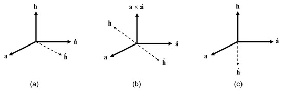
Figure 1. Visual sketch of the geometric conditions that specify the three scenarios considered in our illustrative examples. In (a), since $\mathbf{h}$ and $\dot{\mathbf{h}}$ are not collinear, $a_{\mathrm{H}}<{\left(a_{\mathrm{H}}\right)}_{max}$ (i.e., no saturation). In (b), $\mathbf{h}$ and $\dot{\mathbf{h}}$ are collinear. However, $\mathbf{a}$ and $\mathbf{h}$ are not orthogonal. Therefore, we have in this case $a_{\mathrm{H}}={\left(a_{\mathrm{H}}\right)}_{max}<{\mathcal{A}}_{max}$ (i.e., saturation without maximum). Finally, not only $\mathbf{h}$ and $\dot{\mathbf{h}}$ are collinear in (c). In this scenario, we also have that $\mathbf{a}$ and $\mathbf{h}$ are orthogonal. Therefore, in this case $a_{\mathrm{H}}={\left(a_{\mathrm{H}}\right)}_{max}={\mathcal{A}}_{max}$ (i.e., saturation with maximum). Mutually orthogonal vectors are in bold.

Before discussing our final remarks, we note that Pati reported in Ref. [21] that the quantum acceleration limit saturates in any finite-dimensional Hilbert space where the nonstationary Hamiltonian of the system is given by H$\left(t\right)\stackrel{\mathrm{def}}{=}\lambda \left(t\right){\mathrm{H}}_0$. Here, ${\mathrm{H}}_0$ is a time-independent operator, while $\lambda \left(t\right)$ denotes a time-varying coupling parameter. In our geometric picture for single-qubit evolutions, Pati’s result can be simply explained by noting that since H$\left(t\right)\stackrel{\mathrm{def}}{=}\lambda \left(t\right)\widehat{h}·\mathsf{œ}$ with $\widehat{h}$ being constant in time, the acceleration limit saturates since $\mathbf{h}\left(t\right)\stackrel{\mathrm{def}}{=}\lambda \left(t\right)\widehat{h}$ and $\dot{\mathbf{h}}\left(t\right)$ are collinear vectors.

We are now ready for our summary of the results and final comments.

5. Conclusions

In this paper, we began with a comparative analysis between the derivations of the quantum acceleration limit for arbitrary finite-dimensional quantum systems in a pure state as originally proposed by Pati (Equation (16)) and Alsing–Cafaro (Equation (28)). The visual summary of this analysis appears in Table 1. Then, limiting our attention to the quantum evolution of two-level quantum systems on a Bloch sphere under general time-dependent Hamiltonians, we recast (Equation (35)) the acceleration limit inequality by means of the Bloch vector $\mathbf{a}\left(t\right)$ of the system and of the magnetic field vector $\mathbf{h}\left(t\right)$ that characterizes the (traceless) Hermitian Hamiltonian of the system H$\left(t\right)\stackrel{\mathrm{def}}{=}\mathbf{h}\left(t\right)·\sigma$. We then found the proper geometric conditions in terms of $\mathbf{a}\left(t\right)$, $\mathbf{h}\left(t\right)$, and their temporal derivatives for which the above-mentioned inequality is saturated and the quantum acceleration is maximum. A visual summary of these conditions appears in Table 2. To illustrate these conditions in an explicit manner, we then discussed three illustrative examples. In the first scenario, the quantum acceleration $a_{\mathrm{H}}\left(t\right)$ (Equation (51)) does not reach the value of its upper bound ${\left(a_{\mathrm{H}}\left(t\right)\right)}_{max}$ (Equation (52)) (i.e., no saturation since $a_{\mathrm{H}}\left(t\right)<{\left(a_{\mathrm{H}}\left(t\right)\right)}_{max}$). This first scenario is specified by the relations $\mathbf{a}\left(t\right)·\mathbf{h}\left(t\right)=0$ and $\mathbf{h}\left(t\right)\times \dot{\mathbf{h}}\left(t\right)\ne \mathbf{0}$. In the second scenario, the quantum acceleration $a_{\mathrm{H}}\left(t\right)$ (Equation (55)) reaches the value of its upper bound ${\left(a_{\mathrm{H}}\left(t\right)\right)}_{max}$ (Equation (56)). However, the upper bound ${\left(a_{\mathrm{H}}\left(t\right)\right)}_{max}$ does not assume its maximum value ${\mathcal{A}}_{max}\left(t\right)$ (Equation (56)) (i.e., saturation without maximum, $a_{\mathrm{H}}\left(t\right)={\left(a_{\mathrm{H}}\left(t\right)\right)}_{max}<{\mathcal{A}}_{max}\left(t\right)$). This second scenario is characterized by the conditions $\mathbf{a}\left(t\right)·\mathbf{h}\left(t\right)\ne 0$ and $\mathbf{h}\left(t\right)\times \dot{\mathbf{h}}\left(t\right)=\mathbf{0}$. In the third scenario, the quantum acceleration $a_{\mathrm{H}}\left(t\right)$ (Equation (60)) reaches the value of its upper bound ${\left(a_{\mathrm{H}}\left(t\right)\right)}_{max}$ (Equation (61)). Moreover, the upper bound ${\left(a_{\mathrm{H}}\left(t\right)\right)}_{max}$ achieves its maximum value ${\mathcal{A}}_{max}\left(t\right)$ (Equation (61)) (i.e., saturation with maximum, $a_{\mathrm{H}}\left(t\right)={\left(a_{\mathrm{H}}\left(t\right)\right)}_{max}={\mathcal{A}}_{max}\left(t\right)$). Finally, this third scenario is described by the relations $\mathbf{a}\left(t\right)·\mathbf{h}\left(t\right)=0$ and $\mathbf{h}\left(t\right)\times \dot{\mathbf{h}}\left(t\right)=\mathbf{0}$.

In this paper, the presentation of our illustrative examples was limited to two-level quantum systems in a pure state, despite the fact that our formal derivation of the quantum acceleration limit applies to any finite-dimensional quantum system in a pure state. Therefore, two clear extensions of our work are its explicit application to higher-dimensional systems in a pure state and, in addition, its conceptual generalization to quantum systems in a mixed quantum state. In this basic single-qubit scenario, unlike what occurs in higher-dimensional cases, the notions of Bloch vectors and Bloch spheres have both a neat physical significance and a clear geometric visualization. When shifting from two-level quantum systems to higher-dimensional systems, the physical meaning of the Bloch vector conserves its usefulness. However, its geometric interpretation is less transparent than that achieved for single-qubit quantum systems [43,44,45,46,47,48]. We refer to Ref. [49] for a very helpful discussion on the Bloch vector representations of single-qubit systems, single-qutrit systems, and two-qubit systems by means of Pauli, Gell-Mann, and Dirac matrices, respectively.

Moreover, when transitioning from pure states to mixed quantum states, we have to tackle additional challenges even for lower-dimensional quantum systems. One of the main obstacles (absent for pure states) is the existence of infinitely many distinguishability distances for mixed quantum states [50,51,52,53,54,55,56]. This freedom in the selection of the metric leads to the conclusion that geometric investigations of physical phenomena are still open to metric-dependent interpretations. Despite much progress, given the nonuniqueness of distinguishability distances for mixed states, comprehending the physical importance of employing either metric remains an objective of significant theoretical and applied relevance [57,58,59].

Although our work is purely driven by conceptual interests in quantum physics, we are aware of the fact that the concept of quantum acceleration limits can lead to practical applications in quantum technology. As a matter of fact, upper limits on the speed, the acceleration, and the jerk (i.e., the rate of change of the acceleration) of a quantum evolution can be employed to quantify the complexity and the efficiency of quantum processes [38,60,61,62,63,64] to gauge the cost of controlled quantum evolutions [1,2,65] and to characterize losses when quantum critical behaviors are present [19,20,66]. For the time being, we leave the study of some of these applied aspects of our research to future scientific endeavors.

Appendix B.1. Deriving Equation (30)

We want to derive here the relation ${\sigma }_{\mathrm{H}}^2\stackrel{\mathrm{def}}{=}\mathrm{tr}\left(\rho {\mathrm{H}}^2\right)-{\left[\mathrm{tr}\left(\rho \mathrm{H}\right)\right]}^2={\mathbf{h}}^2-{\left(\mathbf{a}·\mathbf{h}\right)}^2$ exploiting the fact that $\rho \left(t\right)\stackrel{\mathrm{def}}{=}(1/2)\left(\mathbf{1}+\mathbf{a}·\sigma \right)$ and H$\left(t\right)\stackrel{\mathrm{def}}{=}$$h_0\mathbf{1}+\mathbf{h}·\sigma$. For generality, we are assuming $h_0=h_0\left(t\right)\ne 0$. We begin by observing that

$$\begin{array}{cc}\hfill \mathrm{tr}\left(\rho \mathrm{H}\right)& =\mathrm{tr}\left[\left({\displaystyle \frac{\mathbf{1}+\mathbf{a}·\sigma }{2}}\right)\left(h_0\mathbf{1}+\mathbf{h}·\sigma \right)\right]\hfill \\ \hfill & =\mathrm{tr}\left[\left({\displaystyle \frac{\mathbf{1}}{2}}+{\displaystyle \frac{\mathbf{a}·\sigma }{2}}\right)\left(h_0\mathbf{1}+\mathbf{h}·\sigma \right)\right]\hfill \\ \hfill & =\mathrm{tr}\left[{\displaystyle \frac{h_0}{2}}\mathbf{1}+{\displaystyle \frac{1}{2}}\mathbf{h}·\sigma +{\displaystyle \frac{h_0}{2}}\mathbf{a}·\sigma +{\displaystyle \frac{1}{2}}\left(\mathbf{a}·\sigma \right)\left(\mathbf{h}·\sigma \right)\right]\hfill \\ \hfill & ={\displaystyle \frac{h_0}{2}}\mathrm{tr}\left(\mathbf{1}\right)+{\displaystyle \frac{1}{2}}\mathrm{tr}\left(\mathbf{h}·\sigma \right)+{\displaystyle \frac{h_0}{2}}\mathrm{tr}\left(\mathbf{a}·\sigma \right)+{\displaystyle \frac{1}{2}}\mathrm{tr}\left[\left(\mathbf{a}·\sigma \right)\left(\mathbf{h}·\sigma \right)\right],\hfill \end{array}$$

(A16)

that is,

$$\mathrm{tr}\left(\rho \mathrm{H}\right)=h_0+\mathbf{a}·\mathbf{h},$$

(A17)

since $\mathrm{tr}\left(\mathbf{1}\right)=2$, $\mathrm{tr}\left(\mathbf{h}·\sigma \right)=0$, $\mathrm{tr}\left(\mathbf{a}·\sigma \right)=0$, and $\mathrm{tr}\left[\left(\mathbf{a}·\sigma \right)\left(\mathbf{h}·\sigma \right)\right]=2\mathbf{a}·\mathbf{h}$. Let us focus now on the calculation of $\mathrm{tr}\left(\rho {\mathrm{H}}^2\right)$. We have,

$$\begin{array}{cc}\hfill \rho {\mathrm{H}}^2& =\left({\displaystyle \frac{\mathbf{1}+\mathbf{a}·\sigma }{2}}\right){\left(h_0\mathbf{1}+\mathbf{h}·\sigma \right)}^2\hfill \\ \hfill & =\left({\displaystyle \frac{\mathbf{1}}{2}}+{\displaystyle \frac{\mathbf{a}·\sigma }{2}}\right)\left[h_0^2\mathbf{1}+{\left(\mathbf{h}·\sigma \right)}^2+2h_0\left(\mathbf{h}·\sigma \right)\right]\hfill \\ \hfill & =\left[{\displaystyle \frac{h_0^2}{2}}\mathbf{1}+{\displaystyle \frac{1}{2}}{\left(\mathbf{h}·\sigma \right)}^2+h_0\left(\mathbf{h}·\sigma \right)+{\displaystyle \frac{h_0^2}{2}}\left(\mathbf{a}·\sigma \right)+{\displaystyle \frac{1}{2}}\left(\mathbf{a}·\sigma \right){\left(\mathbf{h}·\sigma \right)}^2+h_0\left(\mathbf{a}·\sigma \right)\left(\mathbf{h}·\sigma \right)\right],\hfill \end{array}$$

(A18)

that is,

$$\mathrm{tr}\left(\rho {\mathrm{H}}^2\right)=h_0^2+{∥\mathbf{h}∥}^2+2h_0\left(\mathbf{a}·\mathbf{h}\right),$$

(A19)

since $\mathrm{tr}\left(\mathbf{1}\right)=2$, $\mathrm{tr}\left[{\left(\mathbf{h}·\sigma \right)}^2\right]=2{∥\mathbf{h}∥}^2$, $\mathrm{tr}\left(\mathbf{h}·\sigma \right)=0$, $\mathrm{tr}\left(\mathbf{a}·\sigma \right)=0$, $\mathrm{tr}\left[\left(\mathbf{a}·\sigma \right){\left(\mathbf{h}·\sigma \right)}^2\right]=0$ and, $\mathrm{tr}\left[\left(\mathbf{a}·\sigma \right)\left(\mathbf{h}·\sigma \right)\right]=2\mathbf{a}·\mathbf{h}$. Using Equations (A17) and (A19), we finally arrive at ${\sigma }_{\mathrm{H}}^2={\mathbf{h}}^2-{\left(\mathbf{a}·\mathbf{h}\right)}^2$.

Appendix B.2. Deriving Equation (33)

We wish to obtain the relation ${\left|⟨\left[\mathrm{H},\dot{\mathrm{H}}\right]⟩\right|}^2={\left[\left(\mathbf{a}\times \mathbf{h}\right)·\dot{\mathbf{h}}-\left(\mathbf{a}\times \dot{\mathbf{h}}\right)·\mathbf{h}\right]}^2$ in Equation (33). Recalling that H $\stackrel{\mathrm{def}}{=}$ $h_0\mathbf{1}+\mathbf{h}·\sigma$ and Ḣ $\stackrel{\mathrm{def}}{=}$ ${\dot{h}}_0\mathbf{1}+\dot{\mathbf{h}}·\sigma$ since we assume for generality that $h_0=h_0\left(t\right)\ne 0$, we begin by noting that

$$\begin{array}{cc}\hfill \left[\mathrm{H},\dot{\mathrm{H}}\right]& =\left[h_0\mathbf{1}+\mathbf{h}·\sigma ,{\dot{h}}_0\mathbf{1}+\dot{\mathbf{h}}·\sigma \right]\hfill \\ \hfill & =\left[h_0\mathbf{1},{\dot{h}}_0\mathbf{1}+\dot{\mathbf{h}}·\sigma \right]+\left[\mathbf{h}·\sigma ,{\dot{h}}_0\mathbf{1}+\dot{\mathbf{h}}·\sigma \right]\hfill \\ \hfill & =\left[h_0\mathbf{1},{\dot{h}}_0\mathbf{1}\right]+\left[h_0\mathbf{1},\dot{\mathbf{h}}·\sigma \right]+\left[\mathbf{h}·\sigma ,{\dot{h}}_0\mathbf{1}\right]+\left[\mathbf{h}·\sigma ,\dot{\mathbf{h}}·\sigma \right]\hfill \\ \hfill & =\left[\mathbf{h}·\sigma ,\dot{\mathbf{h}}·\sigma \right]\hfill \\ \hfill & =\left(\mathbf{h}·\sigma \right)\left(\dot{\mathbf{h}}·\sigma \right)-\left(\dot{\mathbf{h}}·\sigma \right)\left(\mathbf{h}·\sigma \right),\hfill \end{array}$$

(A20)

that is,

$$⟨\left[\mathrm{H},\dot{\mathrm{H}}\right]⟩=⟨\left(\mathbf{h}·\sigma \right)\left(\dot{\mathbf{h}}·\sigma \right)-\left(\dot{\mathbf{h}}·\sigma \right)\left(\mathbf{h}·\sigma \right)⟩.$$

(A21)

From Equation (A21), we have that $⟨\left[\mathrm{H},\dot{\mathrm{H}}\right]⟩$ becomes

$$\begin{array}{cc}\hfill ⟨\left[\mathrm{H},\dot{\mathrm{H}}\right]⟩& =\mathrm{tr}\left(\rho \left[\mathrm{H},\dot{\mathrm{H}}\right]\right)\hfill \\ \hfill & =\mathrm{tr}\left[\left({\displaystyle \frac{\mathbf{1}+\mathbf{a}·\sigma }{2}}\right)\left[\mathrm{H},\dot{\mathrm{H}}\right]\right]\hfill \\ \hfill & =\mathrm{tr}\left\{\left({\displaystyle \frac{\mathbf{1}+\mathbf{a}·\sigma }{2}}\right)\left[\left(\mathbf{h}·\sigma \right)\left(\dot{\mathbf{h}}·\sigma \right)-\left(\dot{\mathbf{h}}·\sigma \right)\left(\mathbf{h}·\sigma \right)\right]\right\}\hfill \\ \hfill & ={\displaystyle \frac{1}{2}}\mathrm{tr}\left[\left(\mathbf{h}·\sigma \right)\left(\dot{\mathbf{h}}·\sigma \right)\right]-{\displaystyle \frac{1}{2}}\mathrm{tr}\left[\left(\dot{\mathbf{h}}·\sigma \right)\left(\mathbf{h}·\sigma \right)\right]+\hfill \\ \hfill & +{\displaystyle \frac{1}{2}}\mathrm{tr}\left[\left(\mathbf{a}·\sigma \right)\left(\mathbf{h}·\sigma \right)\left(\dot{\mathbf{h}}·\sigma \right)\right]-{\displaystyle \frac{1}{2}}\mathrm{tr}\left[\left(\mathbf{a}·\sigma \right)\left(\dot{\mathbf{h}}·\sigma \right)\left(\mathbf{h}·\sigma \right)\right]\hfill \\ \hfill & ={\displaystyle \frac{1}{2}}\mathrm{tr}\left[\left(\mathbf{h}·\dot{\mathbf{h}}\right)\mathbf{1}+i\left(\mathbf{h}\times \dot{\mathbf{h}}\right)·\sigma \right]-{\displaystyle \frac{1}{2}}\mathrm{tr}\left[\left(\dot{\mathbf{h}}·\mathbf{h}\right)\mathbf{1}+i\left(\dot{\mathbf{h}}\times \mathbf{h}\right)·\sigma \right]+\hfill \\ \hfill & +{\displaystyle \frac{1}{2}}\mathrm{tr}\left\{\left[\left(\mathbf{a}·\mathbf{h}\right)\mathbf{1}+i\left(\mathbf{a}\times \mathbf{h}\right)·\sigma \right]\left(\dot{\mathbf{h}}·\sigma \right)\right\}-{\displaystyle \frac{1}{2}}\mathrm{tr}\left\{\left[\left(\mathbf{a}·\dot{\mathbf{h}}\right)\mathbf{1}+i\left(\mathbf{a}\times \dot{\mathbf{h}}\right)·\sigma \right]\left(\mathbf{h}·\sigma \right)\right\}\hfill \\ \hfill & =\mathbf{h}·\dot{\mathbf{h}}-\dot{\mathbf{h}}·\mathbf{h}+{\displaystyle \frac{1}{2}}\mathrm{tr}\left\{\left[i\left(\mathbf{a}\times \mathbf{h}\right)·\sigma \right]\left(\dot{\mathbf{h}}·\sigma \right)\right\}-{\displaystyle \frac{1}{2}}\mathrm{tr}\left\{\left[i\left(\mathbf{a}\times \dot{\mathbf{h}}\right)·\sigma \right]\left(\mathbf{h}·\sigma \right)\right\}\hfill \\ \hfill & ={\displaystyle \frac{i}{2}}\mathrm{tr}\left\{\left[\left(\mathbf{a}\times \mathbf{h}\right)·\dot{\mathbf{h}}\right]\mathbf{1}\right\}-{\displaystyle \frac{i}{2}}\mathrm{tr}\left\{\left[\left(\mathbf{a}\times \dot{\mathbf{h}}\right)·\mathbf{h}\right]\mathbf{1}\right\}\hfill \\ \hfill & =i\left[\left(\mathbf{a}\times \mathbf{h}\right)·\dot{\mathbf{h}}-\left(\mathbf{a}\times \dot{\mathbf{h}}\right)·\mathbf{h}\right],\hfill \end{array}$$

(A22)

that is,

$$⟨\left[\mathrm{H},\dot{\mathrm{H}}\right]⟩=i\left[\left(\mathbf{a}\times \mathbf{h}\right)·\dot{\mathbf{h}}-\left(\mathbf{a}\times \dot{\mathbf{h}}\right)·\mathbf{h}\right].$$

(A23)

Then, using Equation (A23), we finally obtain

$${\left|⟨\left[\mathrm{H},\dot{\mathrm{H}}\right]⟩\right|}^2={\left[\left(\mathbf{a}\times \mathbf{h}\right)·\dot{\mathbf{h}}-\left(\mathbf{a}\times \dot{\mathbf{h}}\right)·\mathbf{h}\right]}^2.$$

(A24)

As a side remark, we observe that writing $\mathbf{h}\left(t\right)=h\left(t\right)\widehat{h}\left(t\right)$, we have $\dot{\mathbf{h}}\left(t\right)=\dot{h}\left(t\right)\widehat{h}\left(t\right)+h\left(t\right){\partial }_t\widehat{h}\left(t\right)$. Therefore, we conclude that ${\left|⟨\left[\mathrm{H},\dot{\mathrm{H}}\right]⟩\right|}^2$ in Equation (A24) vanishes when the magnetic field $\mathbf{h}\left(t\right)$ does not change in direction, that is ${\partial }_t\widehat{h}\left(t\right)=\mathbf{0}$ (i.e., $\mathbf{h}\left(t\right)$ and $\dot{\mathbf{h}}\left(t\right)$ are collinear). Moreover, to double check the correctness of Equation (A24), we use brute force to calculate the RHS and LHS of Equation (A24) in an independent manner. Indeed, setting

$$\rho \stackrel{\mathrm{def}}{=}{\displaystyle \frac{1}{2}}\left(\begin{array}{cc}{a}_3& a_1-i{a}_2\\ a_1+i{a}_2& -a_3\end{array}\right),\mathrm{H}\stackrel{\mathrm{def}}{=}\left(\begin{array}{cc}{h}_0+h_3& h_1-i{h}_2\\ h_1+i{h}_2& h_0-h_3\end{array}\right),\mathrm{and}\text{Ḣ}\stackrel{\mathrm{def}}{=}\left(\begin{array}{cc}{d}_3& d_1-i{d}_2\\ d_1+i{d}_2& -d_3\end{array}\right),$$

(A25)

with $\mathbf{a}\stackrel{\mathrm{def}}{=}\left(a_1,a_2,a_3\right)$, $\mathbf{h}\stackrel{\mathrm{def}}{=}\left(h_1,h_2,h_3\right)$, and $\dot{\mathbf{h}}\stackrel{\mathrm{def}}{=}\left(d_1,d_2,d_3\right)$, we have

$${\left|⟨\left[\mathrm{H},\dot{\mathrm{H}}\right]⟩\right|}^2={\left(2a_1{d}_3{h}_2-2a_1{d}_2{h}_3+2a_2{d}_1{h}_3-2a_2{d}_3{h}_1-2a_3{d}_1{h}_2+2a_3{d}_2{h}_1\right)}^2.$$

(A26)

Similarly, employing simple vector algebra, we obtain

$${\left[\left(\mathbf{a}\times \mathbf{h}\right)·\dot{\mathbf{h}}-\left(\mathbf{a}\times \dot{\mathbf{h}}\right)·\mathbf{h}\right]}^2={\left(2a_1{d}_3{h}_2-2a_1{d}_2{h}_3+2a_2{d}_1{h}_3-2a_2{d}_3{h}_1-2a_3{d}_1{h}_2+2a_3{d}_2{h}_1\right)}^2.$$

(A27)

Thus, we conclude that Equation (A24) is correct. With this final remark, we end our discussion here.

References

- Frey, M.R. Quantum speed limits-primer, perspectives, and potential future directions. Quantum Inf. Process. 2016, 15, 3919–3950. [Google Scholar] [CrossRef]
- Deffner, S.; Campbell, S. Quantum speed limits: From Heisenberg’s uncertainty principle to optimal quantum control. J. Phys. A Math. Theor. 2017, 50, 453001. [Google Scholar] [CrossRef]
- Mandelstam, L.; Tamm, I. The uncertainty relation between energy and time in non-relativistic quantum mechanics. J. Phys. USSR 1945, 9, 249–254. [Google Scholar]
- Margolus, N.; Levitin, L.B. The maximum speed of dynamical evolution. Phys. D 1998, 120, 188–195. [Google Scholar] [CrossRef]
- Hörnedal, N.; Allan, D.; Sönnerborn, O. Extensions of the Mandelstam-Tamm quantum speed limit to systems in mixed states. New J. Phys. 2022, 24, 055004. [Google Scholar] [CrossRef]
- Caianiello, E.R. Is there a maximal acceleration? Lett. Nuovo Cimento 1981, 32, 65–70. [Google Scholar] [CrossRef]
- Caianiello, E.R.; Filippo, S.D.; Marmo, G.; Vilasi, G. Remarks on the maximal-acceleration hypothesis. Lett. Nuovo Cimento 1982, 34, 112–114. [Google Scholar] [CrossRef]
- Caianiello, E.R. Maximal acceleration as a consequence of Heisenberg’s uncertainty relations. Lett. Nuovo Cimento 1984, 41, 370–372. [Google Scholar] [CrossRef]
- Pati, A.K. A note on maximal acceleration. Europhys. Lett. 1992, 18, 285. [Google Scholar] [CrossRef]
- Pati, A.K. On the maximal acceleration and the maximal energy loss. Nuovo Cimento B 1992, 107, 895–901. [Google Scholar] [CrossRef]
- Schot, S.H. Jerk: The time rate of change of acceleration. Am. J. Phys. 1978, 46, 1090–1094. [Google Scholar] [CrossRef]
- Eager, D.; Pendrill, A.-M.; Reistad, N. Beyond velocity and acceleration: Jerk, snap and higher derivatives. Eur. J. Phys. 2016, 37, 065008. [Google Scholar] [CrossRef]
- Masuda, S.; Nakamura, K. Acceleration of adiabatic quantum dynamics in electromagnetic fields. Phys. Rev. A 2011, 84, 043434. [Google Scholar] [CrossRef]
- Masuda, S.; Koenig, J.; Steele, G.A. Acceleration and deceleration of quantum dynamics based on inter-trajectory travel with fast-forward scaling theory. Sci. Rep. 2022, 12, 10744. [Google Scholar] [CrossRef] [PubMed]
- Khujakulov, A.; Nakamura, K. Scheme for accelerating quantum tunneling dynamics. Phys. Rev. A 2016, 93, 022101. [Google Scholar] [CrossRef]
- Larrouy, A.; Patsch, S.; Richaud, R.; Raimond, J.M.; Brune, M.; Koch, C.P.; Gleyzes, S. Fast navigation in a large Hilbert space using quantum optimal control. Phys. Rev. X 2020, 10, 02158. [Google Scholar] [CrossRef]
- Kyriakopoulos, K.J.; Saridis, G.N. Minimum jerk path generation. In Proceedings of the IEEE International Conference on Robotics and Automation, Philadelphia, PA, USA, 24–29 April 1988; Volume 1, p. 364. [Google Scholar]
- Shadmehr, R.; Wise, S.P. The Computational Neurobiology of Reaching and Pointing; MIT Press: Cambridge, MA, USA, 2005. [Google Scholar]
- Liu, L.R.; Hood, J.D.; Yu, Y.; Zhang, J.T.; Wang, K.; Lin, Y.W.; Rosenband, T.; Ni, K.K. Molecular assembly of ground-state cooled single atoms. Phys. Rev. X 2019, 9, 021039. [Google Scholar] [CrossRef]
- Matthies, A.J.; Mortlock, J.M.; McArd, L.A.; Raghuram, A.P.; Innes, A.D.; Gregory, P.D.; Bromley, S.L.; Cornish, S.L. Long-distance optical-conveyor-belt transport of ultracold 133Cs and 87Rb atoms. Phys. Rev. A 2024, 109, 023321. [Google Scholar] [CrossRef]
- Pati, A.K. Quantum acceleration limit. arXiv 2023, arXiv:2312.00864. [Google Scholar]
- Alsing, P.M.; Cafaro, C. From the classical Frenet-Serret apparatus to the curvature and torsion of quantum-mechanical evolutions. Part I. Stationary Hamiltonians. Int. J. Geom. Methods Mod. Phys. 2024, 21, 2450152. [Google Scholar] [CrossRef]
- Alsing, P.M.; Cafaro, C. From the classical Frenet-Serret apparatus to the curvature and torsion of quantum-mechanical evolutions. Part II. Nonstationary Hamiltonians. Int. J. Geom. Methods Mod. Phys. 2024, 21, 2450151. [Google Scholar] [CrossRef]
- Alsing, P.M.; Cafaro, C. Upper limit on the acceleration of a quantum evolution in projective Hilbert space. Int. J. Geom. Methods Mod. Phys. 2024, 21, 2440009. [Google Scholar] [CrossRef]
- Heisenberg, W. Über den anschaulichen Inhalt der quanten theoretischen kinematik und mechanik. Z. Phys. 1927, 43, 172–198. [Google Scholar] [CrossRef]
- Kennard, E.H. Zur Quanten mechanik einfacher Bewegungstypen. Z. Phys. 1927, 44, 326–352. [Google Scholar] [CrossRef]
- Roberston, H.P. The uncertainty principle. Phys. Rev. 1929, 34, 163. [Google Scholar]
- Schrödinger, E. Zum Heisenbergschen Unschärfeprinzip. In Sitzungsberichte der Preussischen Akademie der Wissenschaften, Physikalisch-Mathematische Klasse; Akademie der Wissenschaften: Berlin, Germany, 1930; Volume 14, pp. 296–303. [Google Scholar]
- Englert, B.-G. Uncertainty relations revisited. Phys. Lett. A 2024, 494, 129278. [Google Scholar] [CrossRef]
- Nakahara, M. Geometry, Topology, and Physics; Institute of Physics Publishing Ltd.: Bristol, UK, 2003. [Google Scholar]
- Eguchi, T.; Gilkey, P.B.; Hanson, A.J. Gravitation, gauge theories, and differential geometry. Phys. Rep. 1980, 66, 213–393. [Google Scholar] [CrossRef]
- Bohm, A.; Boya, L.J.; Kendrick, B. Derivation of the geometric phase. Phys. Rev. A 1991, 43, 1206. [Google Scholar] [CrossRef]
- Uhlmann, A.; Crell, B. Geometry of state spaces. In Entanglement and Decoherence; Lecture Notes in Physics; Springer: Berlin/Heidelberg, Germany, 2009; Volume 768, p. 1. [Google Scholar]
- Provost, J.P.; Vallee, G. Riemannian structure on manifolds of quantum states. Commun. Math. Phys. 1980, 76, 289–301. [Google Scholar] [CrossRef]
- Mukunda, N.; Simon, R. Quantum kinematic approach to the geometric phase I. General Formalism. Ann. Phys. 1993, 228, 205–268. [Google Scholar] [CrossRef]
- Anandan, J.; Aharonov, Y. Geometry of quantum evolution. Phys. Rev. Lett. 1990, 65, 1697. [Google Scholar] [CrossRef] [PubMed]
- Braunstein, S.L.; Caves, C.M. Statistical distance and the geometry of quantum states. Phys. Rev. Lett. 1994, 72, 3439. [Google Scholar] [CrossRef] [PubMed]
- Uzdin, R.; Günther, U.; Rahav, S.; Moiseyev, N. Time-dependent Hamiltonians with 100% evolution speed efficiency. J. Phys. A Math. Theor. 2012, 45, 415304. [Google Scholar] [CrossRef]
- Sakurai, J.J. Modern Quantum Mechanics; Addison Wesley Publishing Company, Inc.: Boston, MA, USA, 1985. [Google Scholar]
- Hall, B.C. Quantum Theory for Mathematicians; Springer Science+Business Media: New York, NY, USA, 2013. [Google Scholar]
- Cafaro, C.; Rossetti, L.; Alsing, P.M. Curvature of quantum evolutions for qubits in time-dependent magnetic fields. arXiv 2024, arXiv:2408.14233. [Google Scholar]
- Rossetti, L.; Cafaro, C.; Alsing, P.M. Quantifying deviations from shortest geodesic paths together with waste of energy resources for quantum evolutions on the Bloch sphere. arXiv 2024, arXiv:2408.14230. [Google Scholar]
- Jakobczyk, L.; Siennicki, M. Geometry of Bloch vectors in two-qubit system. Phys. Lett. A 2001, 286, 383–390. [Google Scholar] [CrossRef]
- Kimura, G. The Bloch vector for N-level systems. Phys. Lett. A 2003, 314, 339–349. [Google Scholar] [CrossRef]
- Bertlmann, R.A.; Krammer, P. Bloch vectors for qudits. J. Phys. A Math. Theor. 2008, 41, 235303. [Google Scholar] [CrossRef]
- Kurzynski, P. Multi-Bloch vector representation of the qutrit. Quantum Inf. Comp. 2011, 11, 361–373. [Google Scholar] [CrossRef]
- Xie, J.; Zhang, A.; Cao, N.; Xu, H.; Zheng, K.; Poon, Y.T.; Sze, N.S.; Xu, P.; Zeng, B.; Zhang, L. Observing geometry of quantum states in a three-level system. Phys. Rev. Lett. 2020, 125, 150401. [Google Scholar] [CrossRef]
- Eltschka, C.; Huber, M.; Morelli, S.; Siewert, J. The shape of higher-dimensional state space: Bloch-ball analog for a qutrit. Quantum 2021, 5, 485. [Google Scholar] [CrossRef]
- Gamel, O. Entangled Bloch spheres: Bloch matrix and two-qubit state space. Phys. Rev. A 2016, 93, 062320. [Google Scholar] [CrossRef]
- Bures, D. An extension of Kakutani’s theorem on infinite product measures to the tensor product of semifinite ω*-algebras. Trans. Am. Math. Soc. 1969, 135, 199–212. [Google Scholar] [CrossRef]
- Uhlmann, A. The “transition probability” in the state space of a*-algebra. Rep. Math. Phys. 1976, 9, 273–279. [Google Scholar] [CrossRef]
- Hübner, M. Explicit computation of the Bures distance for density matrices. Phys. Lett. A 1992, 163, 239–242. [Google Scholar] [CrossRef]
- Bengtsson, I.; Zyczkowski, K. Geometry of Quantum States; Cambridge University Press: Cambridge, UK, 2006. [Google Scholar]
- Sjöqvist, E. Geometry along evolution of mixed quantum states. Phys. Rev. Res. 2020, 2, 013344. [Google Scholar] [CrossRef]
- Alsing, P.M.; Cafaro, C.; Luongo, O.; Lupo, C.; Mancini, S.; Quevedo, H. Comparing metrics for mixed quantum states: Sjöqvist and Bures. Phys. Rev. A 2023, 107, 052411. [Google Scholar] [CrossRef]
- Hou, X.-Y.; Zhou, Z.; Wang, X.; Guo, H.; Chien, C.C. Local geometry and quantum geometric tensor of mixed states. Phys. Rev. B 2024, 110, 035144. [Google Scholar] [CrossRef]
- Silva, H.; Mera, B.; Paunkovic, N. Interferometric geometry from symmetry-broken Uhlmann gauge group with applications to topological phase transitions. Phys. Rev. B 2021, 103, 085127. [Google Scholar] [CrossRef]
- Da Silva, H.V. Quantum Information Geometry and Applications. Ph.D. Thesis, IT Lisboa, Lisbon, Portugal, 2021. [Google Scholar]
- Mera, B.; Paunkovic, N.; Amin, S.T.; Vieira, V.R. Information geometry of quantum critical submanifolds: Relevant, marginal, and irrelevant operators. Phys. Rev. B 2022, 106, 155101. [Google Scholar] [CrossRef]
- Campaioli, F.; Sloan, W.; Modi, K.; Pollock, F.A. Algorithm for solving unconstrained unitary quantum brachistochrone problems. Phys. Rev. A 2019, 100, 062328. [Google Scholar] [CrossRef]
- Cafaro, C.; Alsing, P.M. Minimum time for the evolution to a nonorthogonal quantum state and upper bound of the geometric efficiency of quantum evolutions. Quantum Rep. 2021, 3, 444–457. [Google Scholar] [CrossRef]
- Cafaro, C.; Alsing, P.M. Complexity of pure and mixed qubit geodesic paths on curved manifolds. Phys. Rev. D 2022, 106, 096004. [Google Scholar] [CrossRef]
- Cafaro, C.; Ray, S.; Alsing, P.M. Complexity and efficiency of minimum entropy production probability paths from quantum dynamical evolutions. Phys. Rev. E 2022, 105, 034143. [Google Scholar] [CrossRef]
- Cafaro, C.; Alsing, P.M. Qubit geodesics on the Bloch sphere from optimal-speed Hamiltonian evolutions. Class. Quantum Grav. 2023, 40, 115005. [Google Scholar] [CrossRef]
- Van Vu, T.; Saito, K. Thermodynamic unification of optimal transport: Thermodynamic uncertainty relation, minimum dissipation, and thermodynamic speed limits. Phys. Rev. X 2023, 13, 011013. [Google Scholar] [CrossRef]
- Araki, T.; Nori, F.; Gneiting, C. Robust quantum control with disorder-dressed evolution. Phys. Rev. A 2023, 107, 032609. [Google Scholar] [CrossRef]
- Hamazaki, R. Limits to fluctuation dynamics. Commun. Phys. 2024, 7, 361. [Google Scholar] [CrossRef]
- Hamazaki, R. Speed limits for macroscopic transitions. PRX Quantum 2022, 3, 020319. [Google Scholar] [CrossRef]
- Chryssomalakos, C.; Flores-Delgado, A.G.; Guzmán-González, E.; Hanotel, L.; Serrano-Ensástiga, E. Curves in quantum state space, geometric phases, and the brachistophase. J. Phys. A Math. Theor. 2023, 56, 285301. [Google Scholar] [CrossRef]
- Chryssomalakos, C.; Flores-Delgado, A.G.; Guzmán-González, E.; Hanotel, L.; Serrano-Ensástiga, E. Speed excess and total acceleration: A kinetical approach to entanglement. arXiv 2024, arXiv:2401.17427. [Google Scholar] [CrossRef]
- Gibilisco, P.; Imparato, D.; Isola, T. A Robertson-type uncertainty principle and quantum Fisher information. Linear Algebra Its Appl. 2008, 428, 1706–1724. [Google Scholar] [CrossRef][Green Version]
- Maccone, L.; Pati, A.K. Stronger uncertainty relations for all incompatible observables. Phys. Rev. Lett. 2014, 113, 260401. [Google Scholar] [CrossRef] [PubMed]
- Nielsen, M.A.; Chuang, I.L. Quantum Computation and Quantum Information; Cambridge University Press: Cambridge, UK, 2000. [Google Scholar]
- Rieffel, E.G.; Polak, W.H. Quantum Computing: A Gentle Introduction; MIT Press: Cambridge, MA, USA, 2011. [Google Scholar]
- Hidary, D. Quantum Computing: An Applied Approach; Springer: Berlin/Heidelberg, Germany, 2019. [Google Scholar]
Disclaimer/Publisher’s Note: The statements, opinions and data contained in all publications are solely those of the individual author(s) and contributor(s) and not of MDPI and/or the editor(s). MDPI and/or the editor(s) disclaim responsibility for any injury to people or property resulting from any ideas, methods, instructions or products referred to in the content. |
© 2024 by the authors. Licensee MDPI, Basel, Switzerland. This article is an open access article distributed under the terms and conditions of the Creative Commons Attribution (CC BY) license (https://creativecommons.org/licenses/by/4.0/).