A Fast and Accurate Numerical Method for Solving Nonlinear Fourth-Order Boundary Value Problems in the Beam Theory

Abstract

In this paper, an efficient computational discretization approach is investigated for nonlinear fourth-order boundary value problems using beam theory. We specifically deal with nonlinear models described by fourth-order boundary value problems. The proposed method is applied on three different types of problems, i.e., the problem when an elastic bearing is non-zero (Case I), the problem under homogeneous boundary conditions of the unknown function and its second derivative (Case II), and the problem with integral boundary conditions (Case III). Moreover, the convergence analysis of the proposed method is provided. Finally, illustrative examples are included to demonstrate the applicability and validity of the technique and the comparison is made with the existing methods to show the efficiency and accuracy of the proposed method.

1. Introduction

Many real world structures like long-span bridges under wind-loading, robot arms, and tall buildings in earthquake zones can be modeled by beam-like elements. As such, beams are fundamental elements of many engineering applications, and a particular field of study in mechanical engineering is the vibration analysis of beams. The vibration of structural systems subject to loads or displacements is an important serviceability design consideration. These vibrations might affect the operation of machinery or cause major problems like cracks in structural systems. Thus, the early detection of the dynamic loading effects is a vital process in structure analysis [1,2]. A powerful and efficient tool in structural vibration analysis can be provided by studying the presented mathematical models for beams. Among the mathematical models, the numerical investigation of differential equations is a reliable technique that can consider many real factors in terms of initial and boundary conditions by incorporating appropriate terms in the equations.

The classical vibration theory is based on the assumption that one end of each bar is free to move in axial direction. In 1950, Woinowsky-Krieger [3] formulated the beam equation in the presence of axial force and investigated the effect of this force on the vibration of hinged bars. A simplified copy of that problem can be obtained by the following configuration. Suppose that $y\left(x\right)$ is the configuration of a deformed beam of unit length caused by a load $f\left(x\right)$, where $f=-v^{\prime }$, and the shear (vertical) force $v=-EI{y}^{\prime \prime \prime }$, where E is Young’s modules of elasticity and I is the inertial moment. Assuming that $EI=1$, one can obtain the following fourth-order boundary value problem:

$$\begin{array}{ccc}& & y^{\left(4\right)}\left(x\right)=f(x,y\left(x\right)),0<x<1,\hfill \\ & & y\left(0\right)=y^{\prime }\left(0\right)=0,\hfill \\ & & y^{\prime \prime }\left(1\right)=0,y^{\prime \prime \prime }\left(1\right)=h\left(y\left(1\right)\right),\hfill \end{array}$$

where $h\in C\left(\mathbb{R}\right)$. In this problem, the bending of an elastic beam of length one on a nonlinear foundation provided by the function f and a clamp on its left side is described [4] (see Figure 1). A thorough examination of the derivatives of $y\left(x\right)$’s physical meaning can be found in certain publications [4,5,6] and is described as follows: the conditions $y\left(0\right)=y^{\prime }\left(0\right)=0$ explain that the beam’s left end is fixed. However, the condition $y^{\prime \prime \prime }\left(1\right)-h\left(y\left(1\right)\right)=0$ or $y^{\prime \prime \prime }\left(1\right)=h\left(y\left(1\right)\right)$ establishes the connection between the vertical force and the displacement $y\left(1\right)$. Moreover, the requirement $y^{\prime \prime }\left(1\right)=0$ indicates that, at $x=1$, there is no bending moment and the beam is supported by the bearing h.

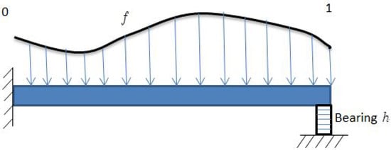
Figure 1. Beam on elastic bearing.

In this study of the beam theory, we encounter some nonlinear fourth-order boundary value problems that take the following general form:

$$\begin{array}{ccc}& & y^{\left(4\right)}\left(x\right)=f(x,y\left(x\right),y^{\prime }\left(x\right),y^{\prime \prime }\left(x\right),y^{\prime \prime \prime }\left(x\right)),0\le x\le L,\hfill \end{array}$$

(1)

$$\begin{array}{ccc}& & \mathit{\psi }(y\left(0\right),y^{\prime }\left(0\right),y^{\prime \prime }\left(0\right),y^{\prime \prime \prime }\left(0\right),y\left(L\right),y^{\prime }\left(L\right),y^{\prime \prime }\left(L\right),y^{\prime \prime \prime }\left(L\right))=\mathbf{0},\hfill \end{array}$$

(2)

where $f\in C^1([0,L]\times {\mathbb{R}}^4)$ and $\mathit{\psi }:{\mathbb{R}}^8\to {\mathbb{R}}^4$ is the boundary function of the problem. This problem extends the analysis of beam vibration to incorporate the bending of elastic beams of length L supported on elastic bearing h and influenced by a nonlinear foundation described by the function f. In particular, we consider Problems (1) and (2) in the following three cases:

Case I: Problem (1) and (2), when an elastic bearing is non-zero;

Case II: Problem (1) and (2) with $L=\pi$, under homogeneous boundary conditions of the unknown function and its second derivative;

Case III: Problem (1) and (2) with integral boundary conditions. In recent years, a number of researchers have proposed approximate methods to solve these problems. For instance, to solve the problem of Case I, we can refer to some iterative methods developed by Ma and Da Silva [6] and Alves et al. [7] and methods such as the quadratic interior penalty [8] and reproducing kernel Hilbert space [4,9]. Also, to solve the problem of Case II, we can refer to the finite-element method developed by Shin [10], Ohm, Lee, and Shin [11], Kim and Shin [12], and the iterative method by Dang and Luan [13]. As well, to solve the problem of Case III, we can refer to the iterative methods developed by Dang and Dang in [14,15]. Of course, it is necessary to mention the point about Case III that some works (see, e.g., [16,17,18,19]) have arisen on this case that have examined only the conditions of the existence of solutions but no methods for finding these solutions have been presented. This paper aims to employ a numerical orthogonal collocation approach utilizing Chebyshev–Gauss–Lobatto (CGL) points to effectively and precisely solve boundary value problems in Cases I, II, and III.

Orthogonal collocation methods, which are part of the collocation approach family, are efficient numerical techniques for finding numerical solutions to a wide range of problems [20,21] and were classically applied in fluid dynamics [22]. A very important point of using these methods is that, if the problem has a smooth solution, then these methods are considered the best tool to solve the problem numerically [23]. Since the boundary value problems of Cases I, II, and III are important problems in the beam theory and, to our knowledge, no attempt has been made to solve them by this class of computational methods, we recommend using the orthogonal collocation method to solve these problems. More specifically, in this paper, we use a Chebyshev orthogonal collocation method that leverages CGL points to transform the solution of the given boundary value problem into a set of nonlinear algebraic equations. It is worth noting that many of the aforementioned methods in solving the boundary value problems of Cases I, II, and III require a large number of iterations, in order to obtain an accurate solution to the problem [5]. However, the Chebyshev orthogonal collocation method gives very accurate results even for small discretization in CGL points and with very low CPU time. Thus, the main contributions and advantages of this work can be summarized as follows:

(i) To the best of our knowledge, this is the first attempt to solve the Case I problem using an orthogonal collocation method. Previous studies have focused on the existence and uniqueness of the solution or used semi-analytical methods to find an approximate solution to this problem, where many iterations are required to obtain an accurate solution to the problem; (ii) In the Case II problem, there are few numerical methods [10,12,13] to solve this problem. One limitation of the existing methods to solve the problem in Case II is the lack of high accuracy in their numerical solutions. However, the proposed numerical method in this study, the Chebyshev orthogonal collocation method, is a reliable method in both accuracy and computational efficiency. In addition, in this instance, the method’s convergence analysis is also provided; (iii) In the Case III problem, this is the second try following the efforts of [14,15] to address the issue. As is seen, the Chebyshev orthogonal collocation method has a very good performance in solving the problem numerically in this case.

The rest of this paper is structured as follows:

Section 2 provides a reformulation of the considered fourth-order boundary value problem to a set of first-order differential equations. The Chebyshev orthogonal collocation method and its application on the obtained system are explained in Section 3, Section 4 and Section 5. Section 6 is devoted to the convergence analysis of the numerical scheme. Some numerical examples of all three cases are investigated in Section 7. Finally, the paper is completed by some concluding remarks.

2. Problem Statement

In this section, we have formulated the nonlinear fourth-order problem in (1)–(2) into a set of first-order differential equations using the substitution provided as follows:

$$\begin{array}{ccc}\hfill & & y_1=y,\hfill \end{array}$$

(3)

$$\begin{array}{ccc}& & y_2=y^{\prime },\hfill \end{array}$$

(4)

$$\begin{array}{ccc}& & y_3=y^{\prime \prime },\hfill \end{array}$$

(5)

$$\begin{array}{ccc}& & y_4=y^{\prime \prime \prime }.\hfill \end{array}$$

(6)

Thus, the fourth-order differential equation in (1) is transferred to the following first-order system of differential equations:

$$\left\{\begin{array}{c}{y}_1^{\prime }\left(x\right)=y_2\left(x\right),\hfill \\ y_2^{\prime }\left(x\right)=y_3\left(x\right),\hfill \\ y_3^{\prime }\left(x\right)=y_4\left(x\right),\hfill \\ y_4^{\prime }\left(x\right)=f(x,y_1\left(x\right),y_2\left(x\right),y_3\left(x\right),y_4\left(x\right)).\hfill \end{array}\right.$$

(7)

Consequently, the boundary function in (2) is changed to the condition

$$\mathit{\psi }(y_1\left(0\right),y_2\left(0\right),y_3\left(0\right),y_4\left(0\right),y_1\left(L\right),y_2\left(L\right),y_3\left(L\right),y_4\left(L\right))=\mathbf{0}.$$

(8)

Obviously, it is possible to express the system of Differential Equation (7) and Boundary Function (8) in vector form:

$$\begin{array}{ccc}& & {\mathbf{y}}^{\prime }\left(x\right)=\mathbf{G}(x,\mathbf{y}\left(x\right)),\hfill \\ & & \mathit{\psi }\left(\mathbf{y}\right(0),\mathbf{y}(L\left)\right)=\mathbf{0},\hfill \end{array}$$

(9)

where $\mathbf{y}\left(x\right)={[y_1\left(x\right),y_2\left(x\right),y_3\left(x\right),y_4\left(x\right)]}^T\in {\mathbb{R}}^4$, and 

$$\mathbf{G}(x,\mathbf{y}\left(x\right))=\left[\begin{array}{c}{y}_2\left(x\right)\\ y_3\left(x\right)\\ y_4\left(x\right)\\ f(x,y_1\left(x\right),y_2\left(x\right),y_3\left(x\right),y_4\left(x\right))\end{array}\right],$$

where $\mathbf{G}:[0,L]\times {\mathbb{R}}^4\to {\mathbb{R}}^4$. In this paper, we will examine the problem (1) and (2) in three general and different cases below

Case I: $y^{\left(4\right)}\left(x\right)=f(x,y\left(x\right),y^{\prime }\left(x\right)),0\le x\le 1$, and  $\left[\begin{array}{c}y\left(0\right)\\ y^{\prime }\left(0\right)\\ y^{\prime \prime }\left(1\right)\\ y^{\prime \prime \prime }\left(1\right)-h\left(y\left(1\right)\right)\end{array}\right]=\mathbf{0}$, where $h\in C\left(\mathbb{R}\right)$;

Case II: $y^{\left(4\right)}\left(x\right)=2y^{\prime \prime }\left(x\right)+{\displaystyle \frac{2y^{\prime \prime }\left(x\right)}{\pi }}\left({\int }_0^{\pi }{\left(y^{\prime }\left(x\right)\right)}^{2}dx\right)+p\left(x\right),0\le x\le \pi$, and $\left[\begin{array}{c}y\left(0\right)\\ y\left(\pi \right)\\ y^{\prime \prime }\left(0\right)\\ y^{\prime \prime }\left(\pi \right)\end{array}\right]=\mathbf{0}$, where $p\left(x\right)$ is a continuous, nonpositive function on the interval $[0,\infty ]$;

Case III: $y^{\left(4\right)}\left(x\right)=f(x,y\left(x\right),y^{\prime }\left(x\right),y^{\prime \prime }\left(x\right),y^{\prime \prime \prime }\left(x\right)),0\le x\le 1$, and $\left[\begin{array}{c}{y}^{\prime }\left(0\right)\\ y^{\prime \prime }\left(0\right)\\ y^{\prime }\left(1\right)\\ y\left(0\right)-{\int }_0^{1}g\left(s\right)y\left(s\right)ds\end{array}\right]=\mathbf{0}$.

     It can be shown that the problems in Case I, Case II, and Case III are simply expressed in the vector forms

Case I: ${\mathbf{y}}^{\prime }\left(x\right)=\mathbf{G}(x,\mathbf{y}\left(x\right))=\left[\begin{array}{c}{y}_2\left(x\right)\\ y_3\left(x\right)\\ y_4\left(x\right)\\ f(x,y_1\left(x\right),y_2\left(x\right))\end{array}\right]$, and $\mathit{\psi }\left(\mathbf{y}\right(0),\mathbf{y}(1\left)\right)$=$\left[\begin{array}{c}{y}_1\left(0\right)\\ y_2\left(0\right)\\ y_3\left(1\right)\\ y_4\left(1\right)-h\left(y_1\left(1\right)\right)\end{array}\right]=\mathbf{0}$;

Case II: ${\mathbf{y}}^{\prime }\left(x\right)=\mathbf{G}(x,\mathbf{y}\left(x\right))=\left[\begin{array}{c}{y}_2\left(x\right)\\ y_3\left(x\right)\\ y_4\left(x\right)\\ 2y_3\left(x\right)\left(1+{\displaystyle \frac{1}{\pi }}{\int }_0^{\pi }{y}_2^2\left(x\right)dx\right)+p\left(x\right)\end{array}\right]$, and $\mathit{\psi }\left(\mathbf{y}\right(0),\mathbf{y}(\pi \left)\right)$=$\left[\begin{array}{c}{y}_1\left(0\right)\\ y_1\left(\pi \right)\\ y_3\left(0\right)\\ y_3\left(\pi \right)\end{array}\right]=\mathbf{0}$;

Case III: ${\mathbf{y}}^{\prime }\left(x\right)=\mathbf{G}(x,\mathbf{y}\left(x\right))=\left[\begin{array}{c}{y}_2\left(x\right)\\ y_3\left(x\right)\\ y_4\left(x\right)\\ f(x,y_1\left(x\right),y_2\left(x\right),y_3\left(x\right),y_4\left(x\right))\end{array}\right]$, and $\mathit{\psi }\left(\mathbf{y}\right(0),\mathbf{y}(1\left)\right)$=$\left[\begin{array}{c}{y}_2\left(0\right)\\ y_3\left(0\right)\\ y_2\left(1\right)\\ y_1\left(0\right)-{\int }_0^{1}g\left(s\right)y_1\left(s\right)ds\end{array}\right]=\mathbf{0}$.

It is noted that the problem in Case I is a nonlinear fourth-order boundary value problem, which models an elastic beam on bearing [5,24,25,26,27,28], and the problems in Case II and Case III are nonlinear fourth-order boundary value problems that arise in the study of the transverse vibrations of a hinged beam [13,29] and flexibility mechanics, chemical engineering, and heat conduction [14]. Fourth-order boundary value problems have application in the mechanics of materials due to their typical representation of the bending behavior of an elastic beam.

3. The Proposed Method for Solving the Boundary Value Problem in Case I

Like all orthogonal collocation methods [22,23,30,31,32], our proposed method has the same properties as those methods. This means that, at first, the method represents the finite approximation of the solution of the problem based on the polynomial interpolation of the solution in some appropriate points; then, the discretization of the target problem begins with the collocation process and, consequently, the target problem is transferred to a set of algebraic equations [33]. For a general view of the proposed method, its flowchart is presented in Figure 2.

Figure 2. Flowchart of the proposed method.

Now, let ${\left\{{\theta }_i\right\}}_{i=1}^n$ denote the CGL points for a certain positive integer n, in which ${\theta }_1=-1$, ${\theta }_n=+1$, and, for $i=2,\dots ,n-1$, ${\theta }_i$ is the i-th root of $(d/dx)T_{n-1}\left(x\right)$, in which $T_{n-1}\left(x\right)$ is the Chebyshev polynomial of the degree $n-1$. It is noted that the celebrated Chebyshev polynomials $T_n,n=0,1,\dots$ are explicitly obtained by the following relations [33]:

$$\begin{array}{ccc}& & T_0\left(x\right)=1,\hfill \\ & & T_1\left(x\right)=x,\hfill \\ & & T_{n+1}\left(x\right)=2x{T}_n\left(x\right)-T_{n-1}\left(x\right),n=1,2,\dots .\hfill \end{array}$$

In addition, the CGL points are also obtained as follows [33]:

$${\theta }_i=-cos\left({\displaystyle \frac{i-1}{n-1}}\pi \right),i=1,\dots ,n.$$

As mentioned, the first step in our proposed method is to approximate the solution of the problem by interpolating the solution on the CGL points. So, in view of the boundary value problem in Case I, we can easily approximate the function $\mathbf{y}$ on the interval $[0,1]$ by

$$\mathbf{y}\left(x\right)\simeq \sum _{i=1}^n\mathbf{y}\left({\widehat{\theta }}_i\right){\widehat{\varphi }}_i\left(x\right)=\sum _{i=1}^n{\mathbf{c}}_i{\widehat{\varphi }}_i\left(x\right),$$

(10)

where ${[c_{1,i},\dots ,c_{4,i}]}^T={\mathbf{c}}_i=\mathbf{y}\left({\widehat{\theta }}_i\right)$ and ${\varphi }_i\left(x\right)$, $i=1,\dots ,n$, are the Lagrange polynomials that are based on ${\left\{{\theta }_i\right\}}_{i=1}^n$, which are established by

$${\varphi }_i\left(x\right)=\prod _{j=1,j\ne i}^n{\displaystyle \frac{x-{\theta }_j}{{\theta }_i-{\theta }_j}},i=1,\dots ,n,$$

and have the Kronecker property

$${\varphi }_i\left({\theta }_j\right)=\left\{\begin{array}{cc}0,\hfill & \mathrm{if}\mathrm{i}\ne \mathrm{j},\hfill \\ 1,\hfill & \mathrm{if}\mathrm{i}=\mathrm{j}.\hfill \end{array}\right.$$

(11)

Also, ${\widehat{\varphi }}_i\left(x\right)={\varphi }_i(2x-1)$ are Lagrange polynomials associated with ${\widehat{\theta }}_i$, and ${\widehat{\theta }}_i=({\theta }_i+1)/2$, $i=1,\dots ,n$ are the moved CGL points on $[0,1]$. Now, in the next step, we discretize the target problem. So, by differentiating from (10) and substituting in the boundary value problem in Case I, we have

$${\mathbf{y}}^{\prime }\left(x\right)\simeq \sum _{i=1}^n{\mathbf{c}}_i{\widehat{\varphi }}_i^{\prime }\left(x\right)\simeq \mathbf{G}(x,\sum _{i=1}^n{\mathbf{c}}_i{\widehat{\varphi }}_i\left(x\right)).$$

(12)

The only remaining process is to collocate the Equation (12) in the CGL points ${\left\{{\widehat{\theta }}_j\right\}}_{j=1}^{n-1}$. So, we have

$$\sum _{i=1}^n{\mathbf{c}}_i{\widehat{\varphi }}_i^{\prime }\left({\widehat{\theta }}_j\right)\simeq \mathbf{G}({\widehat{\theta }}_j,\sum _{i=1}^n{\mathbf{c}}_i{\widehat{\varphi }}_i\left({\widehat{\theta }}_j\right)),j=1,\dots ,n-1,$$

(13)

or

$$\left[\begin{array}{c}\sum _{i=1}^n{c}_{1,i}{\widehat{\varphi }}_i^{\prime }\left({\widehat{\theta }}_j\right)\\ \sum _{i=1}^n{c}_{2,i}{\widehat{\varphi }}_i^{\prime }\left({\widehat{\theta }}_j\right)\\ \sum _{i=1}^n{c}_{3,i}{\widehat{\varphi }}_i^{\prime }\left({\widehat{\theta }}_j\right)\\ \sum _{i=1}^n{c}_{4,i}{\widehat{\varphi }}_i^{\prime }\left({\widehat{\theta }}_j\right)\end{array}\right]\simeq \left[\begin{array}{c}\sum _{i=1}^n{c}_{2,i}{\widehat{\varphi }}_i\left({\widehat{\theta }}_j\right)\\ \sum _{i=1}^n{c}_{3,i}{\widehat{\varphi }}_i\left({\widehat{\theta }}_j\right)\\ \sum _{i=1}^n{c}_{4,i}{\widehat{\varphi }}_i\left({\widehat{\theta }}_j\right)\\ f\left({\widehat{\theta }}_j,\sum _{i=1}^n{c}_{1,i}{\widehat{\varphi }}_i\left({\widehat{\theta }}_j\right),\sum _{i=1}^n{c}_{2,i}{\widehat{\varphi }}_i\left({\widehat{\theta }}_j\right)\right)\end{array}\right],j=1,\dots ,n-1.$$

Now, by using the Kronecker property in (11), Equation (13) is reduced to

$$\left[\begin{array}{c}2\sum _{i=1}^n{c}_{1,i}{d}_{ij}\\ 2\sum _{i=1}^n{c}_{2,i}{d}_{ij}\\ 2\sum _{i=1}^n{c}_{3,i}{d}_{ij}\\ 2\sum _{i=1}^n{c}_{4,i}{d}_{ij}\end{array}\right]=2\sum _{i=1}^n{\mathbf{c}}_i{d}_{ij}\simeq \mathbf{G}({\widehat{\theta }}_j,{\mathbf{c}}_j)=\left[\begin{array}{c}{c}_{2,j}\\ c_{3,j}\\ c_{4,j}\\ f({\widehat{\theta }}_j,c_{1,j},c_{2,j})\end{array}\right],j=1,\dots ,n-1,$$

(14)

where

$$d_{ij}={\varphi }_i^{\prime }\left({\theta }_j\right),i=1,\dots ,n,j=1,\dots ,n-1,$$

is the $(i,j)$-th component of the matrix $\mathbf{D}$, which is named the differentiation matrix. Note that these components are calculated by taking the analytical derivative of ${\left\{{\varphi }_i\left(x\right)\right\}}_{i=1}^n$ and evaluating them at ${\left\{{\theta }_j\right\}}_{j=1}^n$. The following theorem [34] gives the mentioned components of the Chebyshev differentiation matrix.

Theorem 1. 

The components of the $n\times n$ Chebyshev differentiation matrix $\mathbf{D}$ are

$$\begin{array}{ccc}& & d_{11}=-{\displaystyle \frac{2{(n-1)}^2+1}{6}},d_{nn}={\displaystyle \frac{2{(n-1)}^2+1}{6}},\hfill \\ & & d_{jj}=-{\displaystyle \frac{{\theta }_j}{2(1-{\theta }_j^2)}},j=2,\dots ,n-1,\hfill \\ & & d_{ij}={\displaystyle \frac{{\gamma }_i}{{\gamma }_j}}{\displaystyle \frac{{(-1)}^{i+j}}{{\theta }_i-{\theta }_j}},i\ne j,i,j=1,\dots ,n,\hfill \end{array}$$

where

$${\gamma }_k=\left\{\begin{array}{cc}2,\hfill & k=1\mathit{or}n,\hfill \\ 1,\hfill & \mathit{otherwise}.\hfill \end{array}\right.$$

It is clear that the equations in (14) give $4(n-1)$ algebraic equations to determine the unknown vectors ${\mathbf{c}}_i$, along with an additional 4 algebraic equations from the boundary conditions. So, in view of Equation (10), and using the Kronecker property in (11), we have

$$\begin{array}{ccc}& & \mathbf{y}\left(0\right)\simeq \sum _{i=1}^n{\mathbf{c}}_i{\widehat{\varphi }}_i\left({\widehat{\theta }}_1\right)={\mathbf{c}}_1,\hfill \\ & & \mathbf{y}\left(1\right)\simeq \sum _{i=1}^n{\mathbf{c}}_i{\widehat{\varphi }}_i\left({\widehat{\theta }}_n\right)={\mathbf{c}}_n,\hfill \end{array}$$

and, consequently, the four remaining algebraic equations are added to the system of algebraic equations in (14) as

$$\mathit{\psi }({\mathbf{c}}_1,{\mathbf{c}}_n)\simeq \left[\begin{array}{c}{c}_{1,1}\\ c_{2,1}\\ c_{3,n}\\ c_{4,n}-h\left(c_{1,n}\right)\end{array}\right]=\mathbf{0}.$$

(15)

Finally, the $4(n-1)$ collocation equations in (14) and the 4 boundary equations in (15) form a system of nonlinear algebraic equations for obtaining the unknown vectors ${\mathbf{c}}_i$. This system of algebraic equations is represented by

$$\mathbf{0}=\left\{\begin{array}{c}2\sum _{i=1}^n{\mathbf{c}}_i{d}_{i1}-\mathbf{G}({\widehat{\theta }}_1,{\mathbf{c}}_1)\hfill \\ ⋮\hfill \\ 2\sum _{i=1}^n{\mathbf{c}}_i{d}_{i\times (n-1)}-\mathbf{G}({\widehat{\theta }}_{n-1},{\mathbf{c}}_{n-1})\hfill \\ c_{1,1}\hfill \\ c_{2,1}\hfill \\ c_{3,n}\hfill \\ c_{4,n}-h\left(c_{1,n}\right)\hfill \end{array}\right.$$

(16)

After solving the nonlinear system of algebraic equations in (16), the approximate solution to the boundary value problem in Case I is given by

$${\widehat{\mathbf{y}}}_n\left(x\right)\simeq {\left[\sum _{i=1}^n{c}_{1,i}{\widehat{\varphi }}_i\left(x\right),\dots ,\sum _{i=1}^n{c}_{4,i}{\widehat{\varphi }}_i\left(x\right)\right]}^T.$$

4. The Proposed Method for Solving the Boundary Value Problem in Case II

Similarly, the proposed method can be used to discretize the boundary value problem in Case II. However, the difficulty of this problem is rooted in the nonlinear factor within the integral sign [13]. Fortunately, one of the key benefits of the orthogonal collocation methods is in the approximation of an integral with high accuracy. So, assuming that ${\left\{{\tau }_i\right\}}_{i=1}^n$ are the CGL points for a certain positive integer n, we can approximate the integral of a function over the interval $[-1,+1]$ by the n-point Clenshaw–Curtis quadrature rule [33], as 

$${\int }_{-1}^{+1}f\left(x\right)dx\simeq \sum _{i=1}^n{w}_{i}f\left({\tau }_i\right),$$

where ${\left\{w_i\right\}}_{i=1}^n$ are the Clenshaw–Curtis quadrature weights. We refer those interested in how to calculate the weights ${\left\{w_i\right\}}_{i=1}^n$ to the reference [23]. Now suppose that the solution function $\mathbf{y}$ of the boundary value problem in Case II is approximated by Equation (10) on the interval $[0,\pi ]$. Differentiating from (10) and substituting in the boundary value problem in Case II leads to Equation (12). Finally, by collocating Equation (12) in ${\left\{{\widehat{\tau }}_j\right\}}_{j=1}^{n-1}$, we obtain Equation (13), which is expressed by

$$\left[\begin{array}{c}\sum _{i=1}^n{c}_{1,i}{\widehat{\varphi }}_i^{\prime }\left({\widehat{\tau }}_j\right)\\ \sum _{i=1}^n{c}_{2,i}{\widehat{\varphi }}_i^{\prime }\left({\widehat{\tau }}_j\right)\\ \sum _{i=1}^n{c}_{3,i}{\widehat{\varphi }}_i^{\prime }\left({\widehat{\tau }}_j\right)\\ \sum _{i=1}^n{c}_{4,i}{\widehat{\varphi }}_i^{\prime }\left({\widehat{\tau }}_j\right)\end{array}\right]\simeq \left[\begin{array}{c}\sum _{i=1}^n{c}_{2,i}{\widehat{\varphi }}_i\left({\widehat{\tau }}_j\right)\\ \sum _{i=1}^n{c}_{3,i}{\widehat{\varphi }}_i\left({\widehat{\tau }}_j\right)\\ \sum _{i=1}^n{c}_{4,i}{\widehat{\varphi }}_i\left({\widehat{\tau }}_j\right)\\ 2\sum _{i=1}^n{c}_{3,i}{\widehat{\varphi }}_i\left({\widehat{\tau }}_j\right)\left(1+{\displaystyle \frac{1}{\pi }}\sum _{i=1}^n{\widehat{w}}_i{y}_2^2\left({\widehat{\tau }}_i\right)\right)+p\left({\widehat{\tau }}_j\right)\end{array}\right],j=1,\dots ,n-1,$$

where ${\left\{{\widehat{w}}_i\right\}}_{i=1}^n$ are the weights moved to the interval $[0,\pi ]$ by ${\widehat{w}}_i={\displaystyle \frac{\pi }{2}}{w}_i$ and ${\widehat{\tau }}_j={\displaystyle \frac{\pi }{2}}({\tau }_j+1)$. Now, using the Kronecker property from (11), we have

$$\left[\begin{array}{c}2\sum _{i=1}^n{c}_{1,i}{d}_{ij}\\ 2\sum _{i=1}^n{c}_{2,i}{d}_{ij}\\ 2\sum _{i=1}^n{c}_{3,i}{d}_{ij}\\ 2\sum _{i=1}^n{c}_{4,i}{d}_{ij}\end{array}\right]=2\sum _{i=1}^n{\mathbf{c}}_i{d}_{ij}\simeq \mathbf{G}({\widehat{\tau }}_j,{\mathbf{c}}_j)=\left[\begin{array}{c}{c}_{2,j}\\ c_{3,j}\\ c_{4,j}\\ 2c_{3,j}\left(1+{\displaystyle \frac{1}{\pi }}\sum _{i=1}^n{\widehat{w}}_i{y}_2^2\left({\widehat{\tau }}_i\right)\right)+p\left({\widehat{\tau }}_j\right)\end{array}\right],j=1,\dots ,n-1.$$

(17)

In the following, by discretizing the boundary equations of this problem using the Kronecker property in (11), we have

$$\mathit{\psi }({\mathbf{c}}_1,{\mathbf{c}}_n)\simeq \left[\begin{array}{c}{c}_{1,1}\\ c_{1,n}\\ c_{3,1}\\ c_{3,n}\end{array}\right]=\mathbf{0}.$$

(18)

As a result, the system of nonlinear algebraic equations in (17) along with the boundary equation in (18) form the following nonlinear algebraic equations:

$$\mathbf{0}=\left\{\begin{array}{c}2\sum _{i=1}^n{\mathbf{c}}_i{d}_{i1}-\mathbf{G}({\widehat{\tau }}_1,{\mathbf{c}}_1)\hfill \\ ⋮\hfill \\ 2\sum _{i=1}^n{\mathbf{c}}_i{d}_{i\times (n-1)}-\mathbf{G}({\widehat{\tau }}_{n-1},{\mathbf{c}}_{n-1})\hfill \\ c_{1,1}\hfill \\ c_{1,n}\hfill \\ c_{3,1}\hfill \\ c_{3,n}\hfill \end{array}\right.$$

(19)

which should be solved to find the desired ${\mathbf{c}}_i$. Then, the approximate solution to the boundary value problem in Case II is given by

$${\widehat{\mathbf{y}}}_n\left(x\right)\simeq {\left[\sum _{i=1}^n{c}_{1,i}{\widehat{\varphi }}_i\left(x\right),\dots ,\sum _{i=1}^n{c}_{4,i}{\widehat{\varphi }}_i\left(x\right)\right]}^T.$$

5. The Proposed Method for Solving the Boundary Value Problem in Case III

In this case, assuming that ${\left\{{\theta }_i\right\}}_{i=1}^n$ and ${\left\{{\omega }_i\right\}}_{i=1}^n$ are the CGL points and the Clenshaw–Curtis quadrature weights for a certain positive integer n on the interval $[-1,+1]$, respectively. Therefore, the approximate solution $\mathbf{y}$ to the boundary value problem in Case III is determined by Equation (10) on the interval $[0,1]$. Differentiating from (10) and substituting in the boundary value problem in Case III leads to Equation (12). Finally, by collocating Equation (12) in ${\left\{{\widehat{\theta }}_j\right\}}_{j=1}^{n-1}$, we obtain Equation (13), which is expressed by

$$\left[\begin{array}{c}\sum _{i=1}^n{c}_{1,i}{\widehat{\varphi }}_i^{\prime }\left({\widehat{\theta }}_j\right)\\ \sum _{i=1}^n{c}_{2,i}{\widehat{\varphi }}_i^{\prime }\left({\widehat{\theta }}_j\right)\\ \sum _{i=1}^n{c}_{3,i}{\widehat{\varphi }}_i^{\prime }\left({\widehat{\theta }}_j\right)\\ \sum _{i=1}^n{c}_{4,i}{\widehat{\varphi }}_i^{\prime }\left({\widehat{\theta }}_j\right)\end{array}\right]\simeq \left[\begin{array}{c}\sum _{i=1}^n{c}_{2,i}{\widehat{\varphi }}_i\left({\widehat{\theta }}_j\right)\\ \sum _{i=1}^n{c}_{3,i}{\widehat{\varphi }}_i\left({\widehat{\theta }}_j\right)\\ \sum _{i=1}^n{c}_{4,i}{\widehat{\varphi }}_i\left({\widehat{\theta }}_j\right)\\ f\left({\widehat{\theta }}_j,\sum _{i=1}^n{c}_{1,i}{\widehat{\varphi }}_i\left({\widehat{\theta }}_j\right),\sum _{i=1}^n{c}_{2,i}{\widehat{\varphi }}_i\left({\widehat{\theta }}_j\right),\sum _{i=1}^n{c}_{3,i}{\widehat{\varphi }}_i\left({\widehat{\theta }}_j\right),\sum _{i=1}^n{c}_{4,i}{\widehat{\varphi }}_i\left({\widehat{\theta }}_j\right)\right)\end{array}\right],j=1,\dots ,n-1.$$

Now, using the Kronecker property from (11), we have

$$\left[\begin{array}{c}2\sum _{i=1}^n{c}_{1,i}{d}_{ij}\\ 2\sum _{i=1}^n{c}_{2,i}{d}_{ij}\\ 2\sum _{i=1}^n{c}_{3,i}{d}_{ij}\\ 2\sum _{i=1}^n{c}_{4,i}{d}_{ij}\end{array}\right]=2\sum _{i=1}^n{\mathbf{c}}_i{d}_{ij}\simeq \mathbf{G}({\widehat{\theta }}_j,{\mathbf{c}}_j)=\left[\begin{array}{c}{c}_{2,j}\\ c_{3,j}\\ c_{4,j}\\ f({\widehat{\theta }}_j,c_{1,j},c_{2,j},c_{3,j},c_{4,j})\end{array}\right],j=1,\dots ,n-1.$$

(20)

In the following, by discretizing the boundary equations of this problem using the Kronecker property in (11), we have

$$\mathit{\psi }({\mathbf{c}}_1,{\mathbf{c}}_n)\simeq \left[\begin{array}{c}{c}_{2,1}\\ c_{3,1}\\ c_{2,n}\\ c_{1,1}-\sum _{i=1}^n{\widehat{\omega }}_{i}g\left({\widehat{\theta }}_i\right)y_1\left({\widehat{\theta }}_i\right)\end{array}\right]=\mathbf{0},$$

(21)

where ${\left\{{\widehat{\omega }}_i\right\}}_{i=1}^n$ are the weights moved to the interval $[0,1]$ by ${\widehat{\omega }}_i={\displaystyle \frac{1}{2}}{\omega }_i$. As a result, the system of nonlinear algebraic equations in (20) along with the boundary equation in (21) form the following nonlinear algebraic equations

$$\mathbf{0}=\left\{\begin{array}{c}2\sum _{i=1}^n{\mathbf{c}}_i{d}_{i1}-\mathbf{G}({\widehat{\theta }}_1,{\mathbf{c}}_1)\hfill \\ ⋮\hfill \\ 2\sum _{i=1}^n{\mathbf{c}}_i{d}_{i\times (n-1)}-\mathbf{G}({\widehat{\theta }}_{n-1},{\mathbf{c}}_{n-1})\hfill \\ c_{2,1}\hfill \\ c_{3,1}\hfill \\ c_{2,n}\hfill \\ c_{1,1}-\sum _{i=1}^n{\widehat{\omega }}_{i}g\left({\widehat{\theta }}_i\right)y_1\left({\widehat{\theta }}_i\right)\hfill \end{array}\right.$$

(22)

which should be solved to find the desired ${\mathbf{c}}_i$. Then, the approximate solution to the boundary value problem in Case III is given by

$${\widehat{\mathbf{y}}}_n\left(x\right)\simeq {\left[\sum _{i=1}^n{c}_{1,i}{\widehat{\varphi }}_i\left(x\right),\dots ,\sum _{i=1}^n{c}_{4,i}{\widehat{\varphi }}_i\left(x\right)\right]}^T.$$

6. Convergence Analysis

In this section, initially, we discuss certain definitions and lemmas. Afterwards, we provide error bounds for the approximate solutions of the fourth-order differential equations under the Case II type of boundary conditions. Hereafter, let $H_{\omega }^m\left(I\right)$ be a weighted Sobolev space on the reference interval $I=(-1,1)$, a bounded subset of $\mathbb{R}$, where $m\ge 0$ stands for the smoothness order of the solution and the associated weight function for Chebychev methods is $\omega \left(r\right)={(r-r^2)}^{-1/2}$. Then, the norm and semi-norm are defined as

$${\parallel y\left(x\right)\parallel }_{H_{\omega }^m\left(I\right)}={\left(\sum _{i=0}^m\parallel {\displaystyle \frac{{\partial }^i}{\partial x^i}}{y\left(x\right)\parallel }_{L_{\omega }^2}^2\right)}^{{\displaystyle \frac{1}{2}}},{\left|y\left(x\right)\right|}_{H_{\omega }^{m;l}\left(I\right)}={\left(\sum _{i=min(m,l+1)}^m\parallel {\displaystyle \frac{{\partial }^i}{\partial x^i}}{y\left(x\right)\parallel }_{L_{\omega }^2}^2\right)}^{{\displaystyle \frac{1}{2}}}.$$

Here, the  $L_{\omega }^2$ is the space of function for which their weighted $L^2$ norm is finite, with inner product and induced norm defined as follows:

$$\begin{array}{c}\hfill <y\left(x\right),\nu \left(x\right){>}_{\omega }={\int }_{I}y\left(x\right)\nu \left(x\right)\omega \left(x\right)\mathrm{d}x,\hfill \\ \hfill {\parallel y\left(x\right)\parallel }_{L_{\omega }^2\left(I\right)}^2=<y\left(x\right),y\left(x\right){>}_{\omega }.\hfill \end{array}$$

The following lemmas from [30] provide the error bounds for interpolation errors.

Lemma 1. 

Let $I_{n}y\in {\mathbb{P}}_n$ denote the polynomial interpolation of $y\in H_{\omega }^m\left(I\right)$ at Chebychev–Gauss–Lobatto points. Then, the following estimates hold:

$$\begin{array}{ccc}& & \parallel y-I_n{y\parallel }_{L_{\omega }^2\left(I\right)}\le C{n}^{-m}{\left|y\right|}_{H_{\omega }^{m;n}\left(I\right)},\hfill \\ & & \parallel y^{\prime }-{\left(I_{n}y\right)}^{\prime }{\parallel }_{L_{\omega }^2\left(I\right)}\le C{n}^{1-m}{\left|y\right|}_{H_{\omega }^{m;n}\left(I\right)}.\hfill \end{array}$$

Lemma 2. 

Let $\varphi \in {\mathbb{P}}_n$; then, for any integer $r\ge 1$ and $2\le p\le \infty$, there exists a positive constant C such that

$$\parallel {\varphi }^{\left(r\right)}{\parallel }_{L_{\omega }^p\left(I\right)}\le C{n}^{2r}{\parallel \varphi \parallel }_{L_{\omega }^p\left(I\right)}.$$

Now, let us define the following subspaces of ${\mathbb{P}}_n$ as $V_n=H_{\omega }^m\cap {\mathbb{P}}_n$ and

$$V_0=\{\nu \in H_{\omega }^m:\nu \left(0\right)=\nu \left(\pi \right)=0\},V_{n,0}=V_0\cap {\mathbb{P}}_n.$$

From [30], we have the following error bound for the projector $P_{n,0}\in V_{n,0}$:

$$\parallel y-P_{n,0}{y\parallel }_{H_{\omega }^k\left(I\right)}\le C{n}^{k-m}{\left|y\right|}_{H_{\omega }^{m;n}\left(I\right)},\forall y\in H_{\omega }^m,m\ge 1,\mathrm{for}k=0,1.$$

Moreover, one can obtain a polynomial $y_n\in {\mathbb{P}}_{n,0}$ that satisfies

$$\parallel y-y_n{\parallel }_{H_{\omega }^k\left(I\right)}\le C{n}^{k-m}{\left|y\right|}_{H_{\omega }^{m;n}\left(I\right)},\mathrm{for}k=0,1.$$

Theorem 2. 

Consider the first-order system of differential equations in $\left(7\right)$ in general form and its corresponding spectral approximation from $V_n$ or $V_{n,0}$. Suppose that $e_i\left(x\right)=y_i\left(x\right)-P_{n,0}\left(y_i\left(x\right)\right),i=1,3,$ and $e_i\left(x\right)=y_i\left(x\right)-P_n\left(y_i\left(x\right)\right),i=2,4.$ Then, one can obtain

$$\left\{\begin{array}{c}\parallel e_1{\left(x\right)\parallel }_{L_{\omega }^2}\le \widehat{C}{L}^{min(m,n)}{n}^{-m}{\left|y_2\left(x\right)\right|}_{H_{\omega }^{m;n}},\hfill \\ \parallel e_2{\left(x\right)\parallel }_{L_{\omega }^2}\le \widehat{C}{L}^{min(m,n)}{n}^{-m}{\left|y_3\left(x\right)\right|}_{H_{\omega }^{m;n}}\hfill \\ \parallel e_3{\left(x\right)\parallel }_{L_{\omega }^2}\le \widehat{C}{L}^{min(m,n)}{n}^{-m}{\left|y_4\left(x\right)\right|}_{H_{\omega }^{m;n}},\hfill \\ \parallel e_4{\left(x\right)\parallel }_{L_{\omega }^2}\le M\widehat{C}{L}^{min(m,n)}{n}^{-m}\sum _{i=1}^4|y_i{\left(x\right)|}_{H_{\omega }^{m;n}},\hfill \end{array}\right.$$

where $M={min}_{1\le i\le 4}{max}_{x\in [0,L]}\left|f_{y_i}(x,y\left(x\right))\right|$ and $\widehat{C}$ is a constant.

Proof. 

Subtracting the second case of the system of differential equations from its spectral approximation, one can easily obtain

$$\left\{\begin{array}{c}{e}_1^{\prime }\left(x\right)=e_2\left(x\right),\hfill \\ e_2^{\prime }\left(x\right)=e_3\left(x\right),\hfill \\ e_3^{\prime }\left(x\right)=e_4\left(x\right),\hfill \\ e_4^{\prime }\left(x\right)=f(x,y_1,y_2,y_3,y_4)-f(x,P_{n,0}\left(y_1\right),P_n\left(y_2\right),P_{n,0}\left(y_3\right),P_n\left(y_4\right)).\hfill \end{array}\right.$$

Multiplying both sides of each equation of the error system by $e_i\left(x\right)$, and considering the fact that $e_i\left(x\right)$ belongs to $V_{n,0}$, we can obtain

$$\left\{\begin{array}{c}{\displaystyle \frac{d}{dx}}{\parallel e_1^{\prime }\left(x\right)\parallel }_{L_{\omega }^2\left(I\right)}^2=<e_2\left(x\right),e_1\left(x\right){>}_{\omega },\hfill \\ {\displaystyle \frac{d}{dx}}{\parallel e_2^{\prime }\left(x\right)\parallel }_{L_{\omega }^2\left(I\right)}^2=<e_3\left(x\right),e_2\left(x\right){>}_{\omega },\hfill \\ {\displaystyle \frac{d}{dx}}{\parallel e_3^{\prime }\left(x\right)\parallel }_{L_{\omega }^2\left(I\right)}^2=<e_4\left(x\right),e_3\left(x\right){>}_{\omega },\hfill \\ {\displaystyle \frac{d}{dx}}{\parallel e_4^{\prime }\left(x\right)\parallel }_{L_{\omega }^2\left(I\right)}^2=<f(x,y_1,y_2,y_3,y_4)-f(x,P_{n,0}\left(y_1\right),P_n\left(y_2\right),P_{n,0}\left(y_3\right),P_n\left(y_4\right)),e_4\left(x\right){>}_{\omega }.\hfill \end{array}\right.$$

Now, using Cauchy–Schwartz inequality, one can obtain

$$\left\{\begin{array}{c}2\parallel e_i{\left(x\right)\parallel }_{L_{\omega }^2}{\displaystyle \frac{d}{dx}}{\parallel e_i\left(x\right)\parallel }_{L_{\omega }^2}=<e_i\left(x\right),e_{i+1}\left(x\right){>}_{\omega }\hfill \\ \le \parallel e_{i+1}{\left(x\right)\parallel }_{L_{\omega }^2}{\parallel e_i\left(x\right)\parallel }_{L_{\omega }^2},i=1,2,3,\hfill \\ \\ 2\parallel e_4{\left(x\right)\parallel }_{L_{\omega }^2}{\displaystyle \frac{d}{dx}}{\parallel e_4\left(x\right)\parallel }_{L_{\omega }^2}=\hfill \\ <f(x,y_1,y_2,y_3,y_4)-f(x,P_{n,0}\left(y_1\right),P_n\left(y_2\right),P_{n,0}\left(y_3\right),P_n\left(y_4\right)),e_4\left(x\right){>}_{\omega }.\hfill \end{array}\right.$$

Since $f\in C^1([0,\pi ]\times {\mathbb{R}}^4)$, then, by the aid of a first-order Taylor expansion, one can conclude

$$\begin{array}{c}f(x,y_1,y_2,y_3,y_4)-f(x,P_{n,0}\left(y_1\right),P_n\left(y_2\right),P_{n,0}\left(y_3\right),P_n\left(y_4\right))\approx \hfill \\ e_1\left(x\right)f_{y_1}(x,y\left(x\right))+e_2\left(x\right)f_{y_2}(x,y\left(x\right))+e_3\left(x\right)f_{y_3}(x,y\left(x\right))+e_4\left(x\right)f_{y_4}(x,y\left(x\right)).\hfill \end{array}$$

So, we can obtain

$$\begin{array}{c}\hfill <f(x,y_1,y_2,y_3,y_4)-f(x,P_{n,0}\left(y_1\right),P_n\left(y_2\right),P_{n,0}\left(y_3\right),P_n\left(y_4\right)),e_4\left(x\right){>}_{\omega }\hfill \\ \hfill \approx \sum _{i=1}^4<e_i\left(x\right)f_{y_i}(x,y\left(x\right)),e_4\left(x\right){>}_{\omega }.\hfill \end{array}$$

Consequently, if we define $M={min}_{1\le i\le 4}{max}_{x\in [0,L]}\left|f_{y_i}(x,y\left(x\right))\right|$, then

$$\begin{array}{c}2\parallel e_4{\left(x\right)\parallel }_{L_{\omega }^2}{\displaystyle \frac{d}{dx}}{\parallel e_4\left(x\right)\parallel }_{L_{\omega }^2}=\hfill \\ <f(x,y_1,y_2,y_3,y_4)-f(x,P_{n,0}\left(y_1\right),P_n\left(y_2\right),P_{n,0}\left(y_3\right),P_n\left(y_4\right)),e_4\left(x\right){>}_{\omega }\hfill \\ \le \parallel f(x,y\left(x\right)-f(x,\widehat{y}\left(x\right)){\parallel }_{\omega }\parallel e_4\left(x\right){\parallel }_{L_{\omega }^2}\hfill \\ \le \sum _{i=1}^4\parallel e_i\left(x\right)f_{y_i}{(x,y\left(x\right))\parallel }_{\omega }{\parallel e_4\left(x\right)\parallel }_{L_{\omega }^2}\hfill \\ \le M\parallel e_4{\left(x\right)\parallel }_{L_{\omega }^2}\sum _{i=1}^4\parallel e_i{\left(x\right)\parallel }_{L_{\omega }^2}.\hfill \end{array}$$

Eventually, after some simplification and the approximation of error bounds, the latest error can be written as

$$\left\{\begin{array}{c}\parallel e_1{\left(x\right)\parallel }_{L_{\omega }^2}\le \widehat{C}{L}^{min(m,n)}{n}^{-m}{\left|y_2\left(x\right)\right|}_{H_{\omega }^{m;n}},\hfill \\ \parallel e_2{\left(x\right)\parallel }_{L_{\omega }^2}\le \widehat{C}{L}^{min(m,n)}{n}^{-m}{\left|y_3\left(x\right)\right|}_{H_{\omega }^{m;n}}\hfill \\ \parallel e_3{\left(x\right)\parallel }_{L_{\omega }^2}\le \widehat{C}{L}^{min(m,n)}{n}^{-m}{\left|y_4\left(x\right)\right|}_{H_{\omega }^{m;n}},\hfill \\ \parallel e_4{\left(x\right)\parallel }_{L_{\omega }^2}\le M\widehat{C}{L}^{min(m,n)}{n}^{-m}\sum _{i=1}^4|y_i{\left(x\right)|}_{H_{\omega }^{m;n}},\hfill \end{array}\right.$$

and these inequalities complete the proof.    □

From these inequalities, it can be seen that the convergence rate of the proposed scheme is equal to m. So, we can conclude the spectral convergence for the problems with high smoothness order.

7. Numerical Illustrations

In this section, six test examples demonstrate how effective the method is through numerical illustrations. Additionally, to assess the precision of the suggested approach, the maximum absolute error at collocation points is calculated by

$$\begin{array}{ccc}& & \mathrm{Case}\left(\mathbf{I}\right),\left(\mathbf{III}\right):E_n=\underset{1\le k\le n}{max}|{\widehat{y}}_n\left({\widehat{\theta }}_k\right)-y^{*}\left({\widehat{\theta }}_k\right)|,\hfill \\ & & \mathrm{Case}\left(\mathbf{II}\right):E_n=\underset{1\le k\le n}{max}|{\widehat{y}}_n\left({\widehat{\tau }}_k\right)-y^{*}\left({\widehat{\tau }}_k\right)|,\hfill \end{array}$$

where ${\widehat{y}}_n$ is the numerical solution obtained by the proposed method and $y^{*}$ is the analytical solution. Also, to verify the error bounds for the approximate solutions of the fourth-order differential equations under the Case II type of boundary conditions in Theorem 2, the convergence rate of the presented method has also been reported in the test example 3 by

$$\mathrm{Ratio}={\displaystyle \frac{|\ln \left(E_n\right)-\ln \left(E_{n^{\prime }}\right)|}{|\ln \left(n\right)-\ln \left(n^{\prime }\right)|}}.$$

(23)

Furthermore, the computations are conducted on a $2.53$ GHz Core i5 PC Laptop with 4 GB of RAM using Matlab R2016a, and the nonlinear algebraic system (16), (19), or (22) is solved with the Matlab function fsolve. We keep running the fsolve function until the tolerances for function value (TolFun) and parameter value (TolX) drop below ${10}^{-14}$. In addition, we designate one vector as the starting estimate for unknown parameters.

7.1. Test Example 1

Consider the following boundary value problem, which is taken from [5]. The problem is presented by

$$\left\{\begin{array}{c}{y}^{\left(4\right)}\left(x\right)=f(x,y\left(x\right),y^{\prime }\left(x\right))=72x^2-{\displaystyle \frac{2784}{61}}x-{\displaystyle \frac{48}{61}},\hfill \\ h\left(y\left(x\right)\right)={\displaystyle \frac{24sin\left(y\right(x\left)\right)}{61sin\left(\frac{48}{61}\right)}},0\le x\le 1,\hfill \\ y\left(0\right)=y^{\prime }\left(0\right)=y^{\prime \prime }\left(1\right)=0,\hfill \\ y^{\prime \prime \prime }\left(1\right)-h\left(y\left(1\right)\right)=0,\hfill \end{array}\right.$$

and an analytical solution is available thanks to Ma and Da Silva [6] and Geng [9] as $y\left(x\right)={\displaystyle \frac{1}{5}}{x}^6-{\displaystyle \frac{116}{305}}{x}^5-{\displaystyle \frac{2}{61}}{x}^4+x^2$. It is noted that, using Substitutions (3)–(6), the fourth-order differential equation is transferred to the following first-order system of boundary value problems:

$$\left\{\begin{array}{c}{y}_1^{\prime }\left(x\right)=y_2\left(x\right),\hfill \\ y_2^{\prime }\left(x\right)=y_3\left(x\right),\hfill \\ y_3^{\prime }\left(x\right)=y_4\left(x\right),\hfill \\ y_4^{\prime }\left(x\right)=72x^2-{\displaystyle \frac{2784}{61}}x-{\displaystyle \frac{48}{61}},\hfill \\ y_1\left(0\right)=y_2\left(0\right)=y_3\left(1\right)=0,\hfill \\ y_4\left(1\right)-{\displaystyle \frac{24sin\left(y_1\left(1\right)\right)}{61sin\left(\frac{48}{61}\right)}}=0.\hfill \end{array}\right.$$

We now begin addressing this problem utilizing the method that has been outlined. The approximated solution for $n=7$ discretization points alongside the analytical solution and the absolute error function are shown in Figure 3. Also, the maximum absolute errors obtained from the implementation of the proposed method for various values of n with their CPU times, in comparison to the methods developed by Ma and Da Silva [6] and Geng [9] when using five iterates, are reported in Table 1. For better viewing, the log-linear graph of the obtained errors is plotted in Figure 4. They confirm that our proposed method, by using few points in discretization and with very low execution time, has succeeded in obtaining high-accuracy results compared to the existing methods.

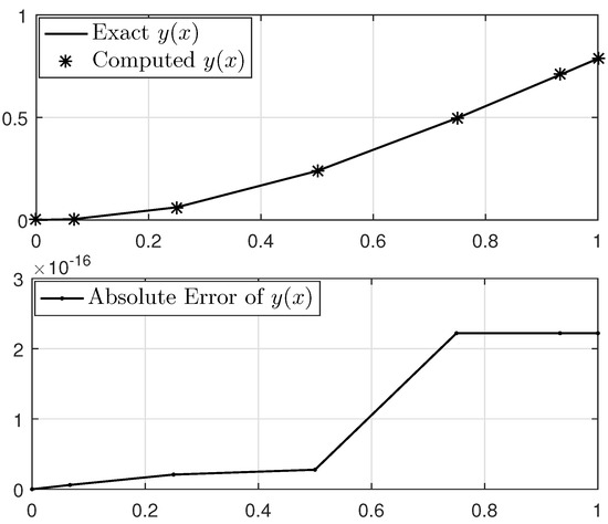
Figure 3. Solution of Example 1 for $n=7$ discretization points.

Table 1. The maximum absolute errors, $E_n$, for different values of n in Example 1.

n	${\mathit{E}}_{\mathit{n}}$	CPU Time (s)
4	1.30 $\times {10}^{-1}$	0.02
5	1.12 $\times {10}^{-3}$	0.03
6	4.88 $\times {10}^{-4}$	0.03
7	2.22 $\times {10}^{-16}$	0.04
8	7.77 $\times {10}^{-16}$	0.05
9	1.11 $\times {10}^{-16}$	0.06
The best result in [6]	8.3914 $\times {10}^{-3}$	Not reported
The best result in [9]	2.7495 $\times {10}^{-3}$	Not reported

Figure 4. The maximum absolute error versus n in Example 1 (log-linear graph).

7.2. Test Example 2

In the second example, we consider the nonlinear boundary value problem, which has been treated in [5]. The problem is presented by

$$\left\{\begin{array}{c}{y}^{\left(4\right)}\left(x\right)=f(x,y\left(x\right),y^{\prime }\left(x\right))={\left(y^{\prime }\right)}^2-{\displaystyle \frac{1}{36}}{x}^6+{\displaystyle \frac{7}{36}}{x}^5-{\displaystyle \frac{9}{16}}{x}^4+{\displaystyle \frac{7}{9}}{x}^3-{\displaystyle \frac{4}{9}}{x}^2+1,0\le x\le 1,\hfill \\ h\left(y\left(x\right)\right)=-{\displaystyle \frac{1}{6}}\sqrt{{\displaystyle \frac{72}{13}}y\left(x\right)},\hfill \\ y\left(0\right)=y^{\prime }\left(0\right)=y^{\prime \prime }\left(1\right)=0,\hfill \\ y^{\prime \prime \prime }\left(1\right)-h\left(y\left(1\right)\right)=0,\hfill \end{array}\right.$$

and has an analytical solution as $y\left(x\right)={\displaystyle \frac{1}{24}}{x}^4-{\displaystyle \frac{7}{36}}{x}^3+{\displaystyle \frac{1}{3}}{x}^2$ [4,7]. It is noted that, using Substitutions (3)–(6), the fourth-order differential equation is transferred to the following first-order system of boundary value problems:

$$\left\{\begin{array}{c}{y}_1^{\prime }\left(x\right)=y_2\left(x\right),\hfill \\ y_2^{\prime }\left(x\right)=y_3\left(x\right),\hfill \\ y_3^{\prime }\left(x\right)=y_4\left(x\right),\hfill \\ y_4^{\prime }\left(x\right)=y_2^2\left(x\right)-{\displaystyle \frac{1}{36}}{x}^6+{\displaystyle \frac{7}{36}}{x}^5-{\displaystyle \frac{9}{16}}{x}^4+{\displaystyle \frac{7}{9}}{x}^3-{\displaystyle \frac{4}{9}}{x}^2+1,\hfill \\ y_1\left(0\right)=y_2\left(0\right)=y_3\left(1\right)=0,\hfill \\ y_4\left(1\right)+{\displaystyle \frac{1}{6}}\sqrt{{\displaystyle \frac{72}{13}}{y}_1\left(1\right)}=0.\hfill \end{array}\right.$$

Now, we start solving the problem using the presented method. The approximated solution for $n=6$ discretization points alongside the analytical solution and the absolute error function are shown in Figure 5. Also, the maximum absolute errors obtained from the implementation of the proposed method for various values of n with their CPU times are reported in Table 2. For better viewing, the log-linear graph of the obtained errors is plotted in Figure 6. Moreover, in Table 3, the maximum absolute error of the proposed method when using just $n=6$ discretization points in comparison with three other methods is given. The outcomes indicate that the method introduced closely approximates the analytical solution with extremely high accuracy.

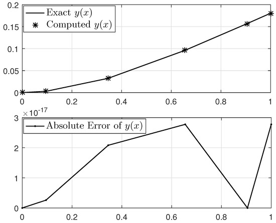
Figure 5. Solution of Example 2 for $n=6$ discretization points.

Table 2. The maximum absolute errors, $E_n$, for different values of n in Example 2.

n	${\mathit{E}}_{\mathit{n}}$	CPU Time (s)
3	4.37 $\times {10}^{-3}$	0.02
4	2.09 $\times {10}^{-3}$	0.02
5	8.33 $\times {10}^{-17}$	0.03
6	2.78 $\times {10}^{-17}$	0.03
7	2.78 $\times {10}^{-17}$	0.03

Figure 6. The maximum absolute error versus n in Example 2 (log-linear graph).

Table 3. Comparison of the maximum absolute errors in Example 2.

The best result in [5]	The best result in [4]	The best result in [7]	The proposed method
1.67 $\times {10}^{-15}$	1.98 $\times {10}^{-11}$	3.30 $\times {10}^{-4}$	2.78 $\times {10}^{-17}$

7.3. Test Example 3

In the third example, the following nonlinear boundary value problem, which is taken from [13], is considered. The problem is presented by

$$\left\{\begin{array}{c}{y}^{\left(4\right)}\left(x\right)=2y^{\prime \prime }\left(x\right)+{\displaystyle \frac{2y^{\prime \prime }\left(x\right)}{\pi }}\left({\int }_0^{\pi }{\left(y^{\prime }\left(x\right)\right)}^{2}dx\right)-4sin\left(x\right),0\le x\le \pi ,\hfill \\ y\left(0\right)=y\left(\pi \right)=0,\hfill \\ y^{\prime \prime }\left(0\right)=y^{\prime \prime }\left(\pi \right)=0,\hfill \end{array}\right.$$

where $y\left(x\right)=-sin\left(x\right)$ is an analytical solution to the problem. It is noted that, using Substitutions (3)–(6), the fourth-order differential equation is transferred to the following first-order system of boundary value problems:

$$\left\{\begin{array}{c}{y}_1^{\prime }\left(x\right)=y_2\left(x\right),\hfill \\ y_2^{\prime }\left(x\right)=y_3\left(x\right),\hfill \\ y_3^{\prime }\left(x\right)=y_4\left(x\right),\hfill \\ y_4^{\prime }\left(x\right)=2y_3\left(x\right)\left(1+{\displaystyle \frac{1}{\pi }}{\int }_0^{\pi }{y}_2^2\left(x\right)dx\right)-4sin\left(x\right),\hfill \\ y_1\left(0\right)=y_1\left(\pi \right)=0,\hfill \\ y_3\left(0\right)=y_3\left(\pi \right)=0.\hfill \end{array}\right.$$

Now, we utilize the proposed method to calculate the numerical solution for this problem. The approximated solution for $n=17$ discretization points alongside the exact solution and the absolute error function are shown in Figure 7. Also, the maximum absolute errors obtained from the implementation of the proposed method for various values of n with their CPU times and ratio are summarized in Table 4 and Table 5. From the theoretical results, we know that the ratio should be proportional to the smoothness order of the exact solution. Since the exact solution is infinitely smooth here, one can easily conclude that the proposed method should have a spectrally convergent scheme for this case. This hypothesis is validated by the gradually increasing ratios reported in Table 4 and Table 5. In addition, Table 6 shows a comparison between the best result obtained for the maximum absolute error of the proposed method and two other methods. For better viewing, the log-linear graph of the obtained errors is also plotted in Figure 8. It is evident that, the proposed method demonstrates exceptional precision.

Figure 7. Solution of Example 3 for $n=17$ discretization points.

Table 4. The maximum absolute errors, $E_n$, and ratio for different values of n in Example 3.

n	${\mathit{E}}_{\mathit{n}}$	CPU Time (s)	Ratio
6	5.07 $\times {10}^{-3}$	0.05	−
8	5.70 $\times {10}^{-5}$	0.09	15.60
10	3.93 $\times {10}^{-7}$	0.11	22.30
12	1.84 $\times {10}^{-9}$	0.13	29.42
14	6.17 $\times {10}^{-12}$	0.14	36.96
16	2.11 $\times {10}^{-14}$	0.21	42.52

Table 5. The maximum absolute errors, $E_n$, and ratio for different values of n in Example 3.

n	${\mathit{E}}_{\mathit{n}}$	CPU Time (s)	Ratio
7	1.84 $\times {10}^{-4}$	0.06	−
9	1.14 $\times {10}^{-6}$	0.09	20.23
11	5.04 $\times {10}^{-9}$	0.12	27.02
13	1.83 $\times {10}^{-11}$	0.13	33.63
15	7.62 $\times {10}^{-14}$	0.18	38.30
17	5.55 $\times {10}^{-16}$	0.21	39.33

Table 6. Comparison of the maximum absolute errors in Example 3.

The best result in [13] using 7 iterates	The best result in [10] using 29 iterates	The proposed method
4.3010 $\times {10}^{-13}$	3.0819 $\times {10}^{-11}$	5.55 $\times {10}^{-16}$

Figure 8. The maximum absolute error versus n in Example 3 (log-linear graph).

7.4. Test Example 4

In the fourth example, the following nonlinear boundary value problem, which is taken from [13], is considered. The problem is presented by

$$\left\{\begin{array}{c}{y}^{\left(4\right)}\left(x\right)=2y^{\prime \prime }\left(x\right)+{\displaystyle \frac{2y^{\prime \prime }\left(x\right)}{\pi }}\left({\int }_0^{\pi }{\left(y^{\prime }\left(x\right)\right)}^{2}dx\right)-x^2,0\le x\le \pi ,\hfill \\ y\left(0\right)=y\left(\pi \right)=0,\hfill \\ y^{\prime \prime }\left(0\right)=y^{\prime \prime }\left(\pi \right)=0.\hfill \end{array}\right.$$

It is noted that, using Substitutions (3)–(6), the fourth-order differential equation is transferred to the following first-order system of boundary value problems:

$$\left\{\begin{array}{c}{y}_1^{\prime }\left(x\right)=y_2\left(x\right),\hfill \\ y_2^{\prime }\left(x\right)=y_3\left(x\right),\hfill \\ y_3^{\prime }\left(x\right)=y_4\left(x\right),\hfill \\ y_4^{\prime }\left(x\right)=2y_3\left(x\right)\left(1+{\displaystyle \frac{1}{\pi }}{\int }_0^{\pi }{y}_2^2\left(x\right)dx\right)-x^2,\hfill \\ y_1\left(0\right)=y_1\left(\pi \right)=0,\hfill \\ y_3\left(0\right)=y_3\left(\pi \right)=0.\hfill \end{array}\right.$$

There is no known analytic solution to this problem. Thus, we start solving it using the presented method. The approximated solutions for $n=15,$ 20, and 25 discretization points are shown in Figure 9. Moreover, Table 7 reports various values of y for different values of n to demonstrate the convergence and accuracy of the proposed method. The table shows that the method presented has a high accuracy.

Figure 9. Solutions to Example 4 for $n=15,20$, and 25 discretization points.

Table 7. Different values of y for various values of n in Example 4.

x	n	$\mathit{y}\left(\mathit{x}\right)$	CPU Time (s)
0	5	−1.92 $\times {10}^{-24}$	0.08
	10	−2.01 $\times {10}^{-30}$	0.11
	15	−8.80 $\times {10}^{-31}$	0.18
1	20	−0.698477080299616	0.22
	25	−0.698477080299615	0.30
	30	−0.698477080299615	0.37
2	20	−0.935182982105999	0.22
	25	−0.935182982105998	0.30
	30	−0.935182982105999	0.37
3	20	−0.177961205799748	0.22
	25	−0.177961205799747	0.30
	30	−0.177961205799747	0.37
$\pi$	5	0	0.08
	10	1.68 $\times {10}^{-30}$	0.11
	15	0	0.18
The best accuracy obtained in [13] for $\Vert {y_k\left(x\right)-y_{k-1}\left(x\right)\Vert }_{\infty }$ is $1.43\times {10}^{-11}$

7.5. Test Example 5

In the fifth example, the following nonlinear boundary value problem, which is taken from [14], is considered. The problem is presented by

$$\left\{\begin{array}{c}{y}^{\left(4\right)}\left(x\right)=-18+{\displaystyle \frac{1}{5}}{y}^2\left(x\right)-{\displaystyle \frac{1}{5}}{({\displaystyle \frac{5}{6}}+x^3-{\displaystyle \frac{3}{4}}{x}^4)}^2,0\le x\le 1,\hfill \\ y^{\prime }\left(0\right)=y^{\prime \prime }\left(0\right)=y^{\prime }\left(1\right)=0,\hfill \\ y\left(0\right)-{\int }_0^{1}4s^{4}y\left(s\right)ds=0,\hfill \end{array}\right.$$

where $y\left(x\right)={\displaystyle \frac{5}{6}}+x^3-{\displaystyle \frac{3}{4}}{x}^4$ is an analytical solution to the problem. It is noted that, using Substitutions (3)–(6), the fourth-order differential equation is transferred to the following first-order system of boundary value problems:

$$\left\{\begin{array}{c}{y}_1^{\prime }\left(x\right)=y_2\left(x\right),\hfill \\ y_2^{\prime }\left(x\right)=y_3\left(x\right),\hfill \\ y_3^{\prime }\left(x\right)=y_4\left(x\right),\hfill \\ y_4^{\prime }\left(x\right)=-18+{\displaystyle \frac{1}{5}}{y}_1^2\left(x\right)-{\displaystyle \frac{1}{5}}{({\displaystyle \frac{5}{6}}+x^3-{\displaystyle \frac{3}{4}}{x}^4)}^2,\hfill \\ y_2\left(0\right)=y_3\left(0\right)=y_2\left(1\right)=0,\hfill \\ y_1\left(0\right)-{\int }_0^{1}4s^4{y}_1\left(s\right)ds=0.\hfill \end{array}\right.$$

Now, we apply the proposed method to obtain the numerical solution to this problem. The approximated solution for $n=10$ discretization points, alongside the exact solution and the absolute error function, is shown in Figure 10. It is noted that the best result reported in [14] using 54 iterates gives maximum absolute error $2.6122\times {10}^{-6}$, while, as can be seen from Figure 10, the maximum absolute error in the proposed method is a factor of ${10}^{-15}$.

Figure 10. Solution to Example 5 for $n=10$ discretization points.

7.6. Test Example 6

In the last example, the following nonlinear boundary value problem, which is taken from [14], is considered. The problem is presented by

$$\left\{\begin{array}{c}{y}^{\left(4\right)}\left(x\right)=-\sqrt{1+y\left(x\right)}-sin\left(y\left(x\right)\right),0\le x\le 1,\hfill \\ y^{\prime }\left(0\right)=y^{\prime \prime }\left(0\right)=y^{\prime }\left(1\right)=0,\hfill \\ y\left(0\right)-{\int }_0^{1}sy\left(s\right)ds=0.\hfill \end{array}\right.$$

It is noted that, using Substitutions (3)–(6), the fourth-order differential equation is transferred to the following first-order system of boundary value problems:

$$\left\{\begin{array}{c}{y}_1^{\prime }\left(x\right)=y_2\left(x\right),\hfill \\ y_2^{\prime }\left(x\right)=y_3\left(x\right),\hfill \\ y_3^{\prime }\left(x\right)=y_4\left(x\right),\hfill \\ y_4^{\prime }\left(x\right)=-\sqrt{1+y_1\left(x\right)}-sin\left(y_1\left(x\right)\right),\hfill \\ y_2\left(0\right)=y_3\left(0\right)=y_2\left(1\right)=0,\hfill \\ y_1\left(0\right)-{\int }_0^{1}s{y}_1\left(s\right)ds=0.\hfill \end{array}\right.$$

This problem has no known analytical solution. Therefore, we start solving it using the presented method. The approximated solutions for $n=10,$ 15, and 20 discretization points are shown in Figure 11. Moreover, Table 8 reports various values of y for different values of n to demonstrate the convergence and accuracy of the proposed method. The table shows that the method presented has a high accuracy.

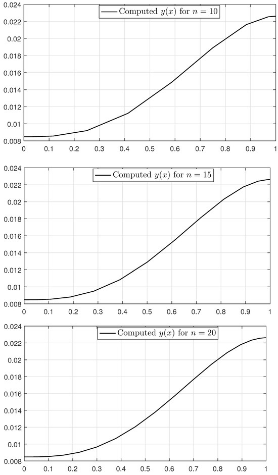
Figure 11. Solutions to Example 6 for $n=10,$ 15, and 20 discretization points.

Table 8. Different values of y for various values of n in Example 6.

x	n	$\mathit{y}\left(\mathit{x}\right)$	CPU Time (s)
0	10	0.008478101111174	0.09
	15	0.008478101110927	0.15
	20	0.008478101110927	0.18
0.25	10	0.009194450655183	0.09
	15	0.009194450654920	0.15
	20	0.009194450654920	0.18
0.5	10	0.012889672995238	0.09
	15	0.012889672994845	0.15
	20	0.012889672994844	0.18
0.75	10	0.018909279622185	0.09
	15	0.018909279621708	0.15
	20	0.018909279621708	0.18
1	10	0.022614795570729	0.09
	15	0.022614795569874	0.15
	20	0.022614795569874	0.18

8. Conclusions

In this paper, a Chebyshev orthogonal collocation method based on using the CGL points was applied for the numerical solution of nonlinear fourth-order boundary value problems using the beam theory. The most important superiorities of the proposed method are as follows: despite using few points in discretization, it has much higher rates of convergence than the existing methods to solve all boundary value problems in Cases I, II, and III; its computer implementation is very simple and fast; and it is a highly precise and effective method for obtaining the numerical solution to these problems. It is noted that, in our previous work [35], another orthogonal collocation method was utilized, together with optimization approaches, to solve the sensitive boundary value problems. However, in this paper, a Chebyshev orthogonal collocation method was chosen for the following reasons: (i) The first is the minimax property of the Chebyshev points [22,33,36]. This implies that the interpolation polynomial constructed on the CGL points will closely resemble the optimal polynomial approximation of the solution in the infinity norm; (ii) Since both the processes of calculating the CGL points and deriving the derivatives of the interpolating polynomials at these points are carried out analytically, the computer implementation of the method will be faster than other orthogonal collocation methods, which use other points such as Legendre–Gauss [37] or Legendre–Gauss–Radau [35], where the mentioned steps would be followed numerically; (iii) Lastly, when the Chebyshev points are utilized for solving the differential equations, the error will be essentially uniform throughout the domain [34]. Moreover, the convergence analysis was performed for the second case and the theoretical and reported numerical results illustrate the spectral convergence in this case. Despite such advantages, similar to spectral methods, the accuracy of the proposed method decreases when dealing with problems that are not smooth or do not have a high order of smoothness. The use of other basis functions such as the family of spline functions in the proposed method to deal with such non-smoothness problems can be utilized as an idea for future works.

References

- Gawali, A.; Sanjay, C.K. Vibration analysis of beams. World Res. J. Civ. Eng. 2011, 1, 15–29. [Google Scholar]
- Han, S.M.; Benaroya, H.; Wei, T. Dynamics of transversely vibrating beams using four engineering theories. J. Sound Vib. 1999, 225, 935–988. [Google Scholar] [CrossRef]
- Woinowsky-Krieger, S. The effect of an axial force on the vibration of hinged bars. J. Appl. Mech. 1950, 17, 35–36. [Google Scholar] [CrossRef]
- Azarnavid, B.; Parand, K.; Abbasbandy, S. An iterative kernel based method for fourth order nonlinear equation with nonlinear boundary condition. Commun. Nonlinear Sci. Numer. Simul. 2018, 59, 544–552. [Google Scholar] [CrossRef]
- Tomar, S.; Singh, M.; Ramos, H.; Wazwaz, A.M. Development of a new iterative method and its convergence analysis for nonlinear fourth-order boundary value problems arising in beam analysis. Math. Methods Appl. Sci. 2022, SI, 1–9. [Google Scholar] [CrossRef]
- Ma, T.F.; Da Silva, J. Iterative solutions for a beam equation with nonlinear boundary conditions of third order. Appl. Math. Comput. 2004, 159, 11–18. [Google Scholar] [CrossRef]
- Alves, E.; Ma, T.F.; Pelicer, M.L. Monotone positive solutions for a fourth order equation with nonlinear boundary conditions. Nonlinear Anal. Theory Methods Appl. 2009, 71, 3834–3841. [Google Scholar] [CrossRef]
- Brenner, S.C.; Gu, S.; Gudi, T.; Sung, L.y. A quadratic C0 interior penalty method for linear fourth order boundary value problems with boundary conditions of the Cahn–Hilliard type. SIAM J. Numer. Anal. 2012, 50, 2088–2110. [Google Scholar] [CrossRef]
- Geng, F. Iterative reproducing kernel method for a beam equation with third-order nonlinear boundary conditions. Math. Sci. 2012, 6, 1–4. [Google Scholar] [CrossRef]
- Shin, J. Finite-element approximation of a fourth-order differential equation. Comput. Math. Appl. 1998, 35, 95–100. [Google Scholar] [CrossRef]
- Ohm, M.R.; Lee, H.Y.; Shin, J. Error estimates of finite-element approximations for a fourth-order differential equation. Comput. Math. Appl. 2006, 52, 283–288. [Google Scholar] [CrossRef]
- Kim, J.; Shin, J. A finite element approximation of a fourth-order boundary value problem. In Proceedings of the Mathematical Optimization Theory and Applications (Proceedings of the Sixth Vietnam-Korea Joint Workshop), Hanoi, Vietnam, 25–29 February 2008; Publishing House for Science and Technology: Hanoi, Vietnam, 2008. [Google Scholar]
- Dang, Q.A.; Luan, V.T. Iterative method for solving a nonlinear fourth order boundary value problem. Comput. Math. Appl. 2010, 60, 112–121. [Google Scholar] [CrossRef]
- Dang, Q.A.; Dang, Q.L. Existence results and iterative method for a fully fourth-order nonlinear integral boundary value problem. Numer. Algorithms 2020, 85, 887–907. [Google Scholar] [CrossRef]
- Dang, Q.A.; Dang, Q.L. Existence results and numerical solution of a fourth-order nonlinear differential equation with two integral boundary conditions. Palest. J. Math. 2023, 12, 174–186. [Google Scholar]
- Zhang, X.; Ge, W. Positive solutions for a class of boundary-value problems with integral boundary conditions. Comput. Math. Appl. 2009, 58, 203–215. [Google Scholar] [CrossRef]
- Li, H.; Wang, L.; Pei, M. Solvability of a fourth-order boundary value problem with integral boundary conditions. J. Appl. Math. 2013, 782363, 1–7. [Google Scholar] [CrossRef]
- Lv, X.; Wang, L.; Pei, M. Monotone positive solution of a fourth-order BVP with integral boundary conditions. Bound. Value Probl. 2015, 2015, 172. [Google Scholar] [CrossRef]
- Benaicha, S.; Haddouchi, F. Positive solutions of a nonlinear fourth-order integral boundary value problem. Ann. West Univ. Timis.-Math. Comput. Sci. 2016, 54, 73–86. [Google Scholar] [CrossRef][Green Version]
- Heydari, M.H.; Avazzadeh, Z. Chebyshev–Gauss–Lobatto collocation method for variable-order time fractional generalized Hirota–Satsuma coupled KdV system. Eng. Comput. 2022, 38, 1835–1844. [Google Scholar] [CrossRef]
- Heydari, M.; Avazzadeh, Z. Jacobi–Gauss–Lobatto collocation approach for non-singular variable-order time fractional generalized Kuramoto–Sivashinsky equation. Eng. Comput. 2022, 38, 925–937. [Google Scholar] [CrossRef]
- Canuto, C.; Hussaini, M.; Quarteroni, A.; Zang, T. Spectral Methods in Fluid Dynamics; Springer Series in Computational Physics; Springer: Berlin/Heidelberg, Germany, 1991. [Google Scholar]
- Trefethen, L.N. Spectral Methods in MATLAB; SIAM: Philadelphia, PA, USA, 2000. [Google Scholar]
- Bai, Z. The upper and lower solution method for some fourth-order boundary value problems. Nonlinear Anal. Theory Methods Appl. 2007, 67, 1704–1709. [Google Scholar] [CrossRef]
- Webb, J.; Infante, G.; Franco, D. Positive solutions of nonlinear fourth-order boundary-value problems with local and non-local boundary conditions. Proc. R. Soc. Edinb. Sect. A Math. 2008, 138, 427–446. [Google Scholar] [CrossRef]
- Li, Y. Two-parameter nonresonance condition for the existence of fourth-order boundary value problems. J. Math. Anal. Appl. 2005, 308, 121–128. [Google Scholar] [CrossRef][Green Version]
- Liu, B. Positive solutions of fourth-order two point boundary value problems. Appl. Math. Comput. 2004, 148, 407–420. [Google Scholar] [CrossRef]
- Zhang, X. Existence and iteration of monotone positive solutions for an elastic beam equation with a corner. Nonlinear Anal. Real World Appl. 2009, 10, 2097–2103. [Google Scholar] [CrossRef]
- Feireisl, E. Exponential attractors for non-autonomous systems: Long-time behaviour of vibrating beams. Math. Methods Appl. Sci. 1992, 15, 287–297. [Google Scholar] [CrossRef]
- Canuto, C.; Hussaini, M.Y.; Quarteroni, A.; Zang, T.A. Spectral Methods: Fundamentals in Single Domains; Springer: Berlin/Heidelberg, Germany, 2007. [Google Scholar]
- Fornberg, B. A Practical Guide to Pseudospectral Methods; Cambridge University Press: Cambridge, UK, 1998. [Google Scholar]
- Shen, J.; Tang, T.; Wang, L. Spectral Methods: Algorithms, Analysis and Applications; Springer Series in Computational Mathematics; Springer: Berlin/Heidelberg, Germany, 2011. [Google Scholar]
- Gautschi, W. Orthogonal Polynomials: Computation and Approximation; Oxford University Press: Oxford, UK, 2004. [Google Scholar]
- Gheorghiu, C.I. Spectral Methods for Differential Problems; Casa Cărtii de Stiintă: Cluj-Napoca, Romania, 2007. [Google Scholar]
- Mehrpouya, M.A.; Salehi, R. A numerical scheme based on the collocation and optimization methods for accurate solution of sensitive boundary value problems. Eur. Phys. J. Plus 2021, 136, 909. [Google Scholar] [CrossRef]
- Atkinson, K. An Introduction to Numerical Analysis, 2nd ed.; Wiley: Hoboken, NJ, USA; India Pvt. Limited: Noida, India, 2008. [Google Scholar]
- Mehrpouya, M.A.; Peng, H. A robust pseudospectral method for numerical solution of nonlinear optimal control problems. Int. J. Comput. Math. 2021, 98, 1146–1165. [Google Scholar] [CrossRef]
Disclaimer/Publisher’s Note: The statements, opinions and data contained in all publications are solely those of the individual author(s) and contributor(s) and not of MDPI and/or the editor(s). MDPI and/or the editor(s) disclaim responsibility for any injury to people or property resulting from any ideas, methods, instructions or products referred to in the content. |
© 2024 by the authors. Licensee MDPI, Basel, Switzerland. This article is an open access article distributed under the terms and conditions of the Creative Commons Attribution (CC BY) license (https://creativecommons.org/licenses/by/4.0/).