Spectral Properties of Exact Polarobreathers in Semiclassical Systems

Abstract

In this paper, we study the spectral properties of polarobreathers, that is, breathers carrying charge in a one-dimensional semiclassical model. We adapt recently developed numerical methods that preserve the charge probability at every step of time integration without using the Born–Oppenheimer approximation, which is the assumption that the electron is not at equilibrium with the atoms or ions. We develop an algorithm to obtain exact polarobreather solutions. The properties of polarobreathers, both stationary and moving ones, are deduced from the lattice and charge variable spectra in the frequency–momentum space. We consider an efficient approach to produce approximate polarobreathers with long lifespans. Their spectrum allows for the determination of the initial conditions and the necessary parameters to obtain numerically exact polarobreathers. The spectra of exact polarobreathers become extremely simple and easy to interpret. We also solve the problem that the charge frequency is not an observable, but the frequency of the charge probability certainly is an observable.

1. Introduction

The subject of a charge moving when coupled to a lattice vibration has a long history [1,2]. This phenomenon is very different from Ohmic conductivity in metals and semiconductors, where electrons in the conduction band or holes in the valence band move freely within a crystal. In insulators, where all the bands are either occupied or empty, but also in metals and semiconductors, an extra charge outside the bands may be attached to some atom or ion and have a low probability of moving to another position. The deformation it produces in the lattice can travel, and is known as a polaron [3,4,5]. The charge—electron, or hole—changes its position to the same state in a neighboring atom. Polarons were first conceived as either a static solution or coupled to phonons, which were set in motion by an external electric field, but there are other possibilities as explained below. There is a probability that a charge may change to the neighboring site due to the overlapping of the electron wavefunctions in each atom, described by the transfer integral. It is clear that if the distance between atoms decreases, there will be an increase in the transition probability, and vice versa. Even for a symmetric vibration, the increase in the transition probability is much larger for shorter distances than the other way around, leading to an exponential dependence on the change in the potential barrier [6].

The level of description in which an electron or hole can be ascribed to a single atom is called the tight-binding approximation. It allows for a semiclassical treatment, in which the heavier atoms are described classically and the much lighter electron is described as a quantum particle. A system can be described in terms of the atomic states, and the quantum Hamiltonian is expressed in terms of the energies of these states and the transfer matrices; the latter often depend on the distance exponentially.

Large displacements of the atoms or ions in a crystal imply that the linear description is no longer valid. This nonlinearity may lead to the apparition of localized entities or, when traveling, solitary waves. Notable examples at the macroscopic scale are tsunamis, which travel thousands of kilometers at jet speed in a different manner to usual sea waves. Only slightly less impressive are tidal bores, solitary waves that travel upriver when the incoming tide encounters the outcoming one. Moreover, rogue waves in the sea appearing apparently from nowhere have been proven to exist by systematic satellite observations.

These solitary waves can be kinks, solitons [7,8], or breathers, also called intrinsic localized modes [9,10,11]. Solitons and kinks have a constant profile in the moving frame, where solitons become zero at $\pm \infty$, while kinks only at one of $\pm \infty$, and tend to a constant at the other infinity. Breathers also have a vibrating profile. Sometimes the distinction depends on the variables used. Important steps in breather theory were the mathematical proof of their existence [12,13] and Floquet and band theory for breathers [14,15,16], which later expanded to dark breathers [17,18] and multibreathers [19,20]. They have been obtained with classical molecular dynamics [21,22] and ab initio molecular dynamics [23,24]. Recently, the spectral theory of exact moving breathers was developed, showing that breathers admit a very simple description in their moving frame, where they have usually a single frequency [25,26]. On the one hand, this makes possible the interpretation of numerical spectra, and on the other, it facilitates the integration methods.

The large displacements bringing neighboring atoms closer and increasing the probability of charge transfer between atoms in semiclassical systems lead to a strong coupling between charge and vibrations. The combined entities are called polarobreathers [27,28,29], or solectrons in some systems [30,31]. The mathematical methods are often within the Born–Oppenheimer approximation [32], that is, supposing that the electrons are always in an equilibrium state with the configuration of atoms around them, due to their dynamics being much faster than the dynamics of the atoms. The authors have overcome this limitation by developing efficient numerical methods for semiclassical systems, based on splitting methods that conserve the charge probability at each step of time integration [33]. On the experimental side of polarobreathers, it was recently discovered that by bombarding layered silicates and other materials with alpha particles, it was possible to measure electrical currents in the absence of an electric field; the electrons or holes were carried by nonlinear lattice excitations [34,35].

The purpose of this paper is to apply the theory of exact polarobreathers in their moving frame to a semiclassical system, using numerical integration methods developed in Ref. [33]. In this way, we clarify the polarobreather spectra, facilitate their description, develop the mathematical methods for obtaining numerically exact polarobreathers, and compare their spectra with the approximate ones. The results can help to identify bands in the spectra of some materials where nonlinear vibrations couple to nonfree charges. The lattice part of the model without the charge is given by a Frenkel–Kontorova model [36,37] with the Lennard-Jones interaction potential, because it has been proven extremely good for producing long-lived breathers in two-dimensional systems [38,39].

The layout of the article is as follows. Section 2 presents the semiclassical system and its transformation into a Hamiltonian one. Section 3 deals with an important problem of the charge description: that the charge frequencies are not an observable of the system. In Section 4, a review of the theory of exact traveling excitations is presented. The linearization of the system is performed in Section 5. Very useful calculations, known as tail analysis, which advance many properties of nonlinear excitations, are presented in Section 6 and Section 7 for stationary and moving polarobreathers, respectively. In Section 8, the developed numerical methods to solve dynamical equations and obtain exact polarobreathers are described. Section 9 and Section 10 analyze stationary and moving polarobreathers, respectively, following a similar pattern: generation, description of the spectrum of approximate polarobreathers, obtainment of exact solutions and interpretation of their spectra, stability analysis, and path continuation. The article ends with the conclusions.

2. The Model

We consider a model of N particles, atoms or ions, with a classical and a quantum Hamiltonian imposing periodic boundary conditions. The classical Hamiltonian is given by

$$H_L=K_E+U_E+V_E=\sum _{n=1}^N\left(\frac{1}{2}{p}_n^2+U\left(u_n\right)+V(1+u_{n+1}-u_n)\right).$$

(1)

In this equation, the variable $u_n$ is the separation of the particle n from the equilibrium position using the lattice unit as length unit; $p_n$ represents the momentum of the particle n, $p_n=m{v}_n=m{\dot{u}}_n$ equal to $p_n={\dot{u}}_n$ because the mass of the particle is chosen as the mass unit. Therefore, $K_E={\sum }_{n=1}^N\frac{1}{2}{p}_n^2$ is the kinetic energy of the system. $U_E={\sum }_{n=1}^{N}U\left(u_n\right)$, is the sum of the on-site energies of the classical system with respect to their equilibrium positions. It represents the interaction of the system with other systems, as other layers in silicates, or simply other atom chains in a crystal. Due to the periodicity of the crystal, the simplest form for the on-site energy for a particle is given by the first-order Fourier series, with the condition that $u_n=0$ is a stable equilibrium with zero energy: $U\left(u_n\right)=U_0(1-cos\left({\omega }_0{u}_n\right))$, known as the Frenkel–Kontorova model. The depth of the potential well is taken as unit of energy, i.e., $U_0=1$, and the period $T_0$ of small oscillations of a particle in the potential well $U\left(u_n\right)$ is taken as time unit, i.e., ${\omega }_0=2\pi$. The interaction energy $V_E={\sum }_{n=1}^{N}V(1+u_{n+1}-u_n)$ is the sum of interaction energies between the particles of the system, that is, the energy of the interaction of the system with itself, described as pairs of Lennard-Jones potential between nearest neighbors. The Lennard-Jones potential has the generic physical property of growing to infinity when the distance between particles becomes zero and tending to a constant value, i.e., with zero derivative or zero force, when the particles separate. The Lennard-Jones potential is given by:

$$V\left(r\right)=\epsilon \left({\left(\frac{\sigma }{r}\right)}^{12}-2{\left(\frac{\sigma }{r}\right)}^6\right).$$

The interaction potential has a minimum at $r=\sigma$ with depth $\epsilon$, being the ratio between the interaction energy and the on-site energy. We use $\epsilon =0.05$, a value that brings about the extraordinary mobility of breathers, both in the system without charge [38,39] and with it [33]. We consider $\sigma =1$, that is, also equal to the lattice constant, which is justified by the fact that there are no forces on the lattice particles at the equilibrium position. We also add the well depth $\epsilon$ to the interaction potential in order to have zero energy at the equilibrium distance.

The quantum Hamiltonian [40] for an electron or hole added to the system is given by:

$${\widehat{H}}_c=\sum _{n=1}^N\left(E_n|n⟩⟨n|-J(u_{n+1}-u_n)\left[|n⟩⟨n+1|+|n+1⟩⟨n|\right]\right),$$

(2)

with the expectation value:

$$H_c=\sum _{n=1}^N\left(E_n{c}_n^{*}{c}_n-J(u_{n+1}-u_n)\left[c_n^{*}{c}_{n+1}+c_{n+1}^{*}{c}_n\right]\right),$$

(3)

which is real, since $c_n^{*}{c}_{n+1}+c_{n+1}^{*}{c}_n=2\mathrm{Re}\left(c_n^{*}{c}_{n+1}\right)$.

$|c_n{|}^2=c_n^{*}{c}_n$ is the probability that the charge is located at site n with energy $E_n$, and the sum of probabilities adds to one, i.e.,

$$\sum _{n=1}^N{\left|c_n\right|}^2=1.$$

(4)

The complex variable $c_n$ is the n-th component of $|\psi ⟩={\sum }_n{c}_n|n⟩$, where |n⟩ represents the state for which the charge is completely localized at site n. The possibility of expanding the wave function in a basis of localized states |n⟩, that is, states for which the electron is tight-bound to a single atom of the system, consists of the tight-binding approximation.

The evolution of the wave function ${\displaystyle |\psi ⟩}$ is described by the Schrödinger equation $\mathrm{i}\hslash {\partial }_t|\psi ⟩={\widehat{H}}_c|\psi ⟩$. The Hamiltonian ${\widehat{H}}_c$ in (2), acting on $|\psi ⟩={\sum }_m{c}_m|m⟩$, leads to:

$${\widehat{H}}_c\sum _m{c}_m|m⟩=\sum _{n,m}{E}_n|n⟩⟨n|c_m|m⟩-J(u_{n+1}-u_n)\left[|n⟩⟨n+1|c_m|m⟩+|n+1⟩⟨n|c_m|m⟩\right],$$

where $⟨n|c_m|m⟩=c_n{\delta }_{n,m}$. The left hand side of the Schrödinger equation becomes $\mathrm{i}\hslash {\partial }_t|\psi ⟩={\sum }_n\mathrm{i}\hslash {\dot{c}}_n|n⟩$. Identifying the components on the basis of vectors $\{|n⟩\}$ in both sides of the evolution equation, we obtain the following evolution equation for the probability amplitudes $c_n$’s:

$$\mathrm{i}\tau {\dot{c}}_n=E_n{c}_n-J(u_{n+1}-u_n)c_{n+1}-J(u_n-u_{n-1})c_{n-1},$$

(5)

where $\tau$ is the reduced Planck constant $\hslash =h/2\pi$ in scaled units, with h being the Planck constant. In Refs. [25,41], which study a particular model for the movement of potassium ions in a silicate layer, the scaled units for length, energy, mass, and time are $u_L=5.19$ Å, the interatomic distance; $u_E=k_e{e}^2/u_L\simeq 2.77$ eV, the electric potential energy between two ions with unit charge e; $u_M=39.1$ amu, the mass of an ion; and $u_T={(u_M{u}_L^2/u_E)}^{1/2}\simeq 0.2$ ps, the derived unit from the previous ones. In those units, $\tau =\hslash /u_E{u}_T\simeq$ 0.00119. In this article, we do not refer to a specific model, but we use $\tau =0.001$ to have a correct order of magnitude. Note that the ratio of masses between a proton and an electron, approximately 2000, is coherent with the fastest movement of the electron with respect to the atoms in the lattice by a factor of $1/\tau$.

Equation (3) is the expected value of the Hamiltonian ${\widehat{H}}_c$ (2) when the system is in the state $|\psi ⟩={\sum }_n{c}_n|n⟩$, i.e., $H_c=⟨\psi |{\widehat{H}}_c|\psi ⟩$. ${\widehat{H}}_c$ is represented on the basis of |n⟩ by a matrix with elements $⟨n|{\widehat{H}}_c|m⟩$. $E_n=⟨n|{\widehat{H}}_c|n⟩$ are, therefore, the diagonal elements. The off-diagonal matrix elements, also called the transfer matrix elements, are $J_{m,n}=⟨m|{\widehat{H}}_c|n⟩$, and are related with the probability of transition between the sites n and m. We suppose that they are zero, except for the nearest-neighbor particles, and that they depend on the distance between particles in the form:

$$\begin{array}{cc}\hfill J_{n+1,n}=& J(u_{n+1}-u_n)=J_{0}exp(-\alpha [1+u_{n+1}-u_n])\hfill \\ \hfill =& I_{0}exp(-\alpha [u_{n+1}-u_n]),\mathrm{with}{I}_0=J_{0}exp(-\alpha ).\hfill \end{array}$$

(6)

Therefore, the transfer elements and the probability of transition between sites increase rapidly when the particles become closer. The parameter values are $\alpha =15$, a value corresponding to the $n=3$ orbitals; and $I_0=J_{0}exp(-\alpha )=5\times {10}^{-4}$, a good value for an insulator at equilibrium. Both values are also very convenient for producing traveling polarobreathers [33]. $E_n$ represents the charge energy at the n-th site, and in general, it may depend on the variables of the lattice. We keep it in the general notation, but in the present paper, we consider it uniform and constant, which makes possible to set it to zero. However, the nonzero value is useful, as explained below in Section 3.

The expected Hamiltonian for the lattice and the charge is given by $H=H_L+H_c$, with Hamiltonian equations for the lattice variables:

$$\begin{array}{c}\hfill {\dot{u}}_n=p_n \mathrm{and} {\dot{p}}_n=-\frac{\partial H}{\partial u_n}.\end{array}$$

(7)

Therefore, the system of governing mathematical equations of the charge–lattice interactions reads as:

$$\begin{array}{} & \hfill {\ddot{u}}_n=& -U^{\prime }\left(u_n\right)+V^{\prime }(1+u_{n+1}-u_n)-V^{\prime }(1+u_n-u_{n-1})\hfill \mathrm{(8)}& & -J^{\prime }(u_{n+1}-u_n)\left(c_n^{*}{c}_{n+1}+c_{n+1}^{*}{c}_n\right)+J^{\prime }(u_n-u_{n-1})\left(c_{n-1}^{*}{c}_n+c_n^{*}{c}_{n-1}\right),\hfill \mathrm{(9)}& \hfill \mathrm{i}\tau {\dot{c}}_n=& E_n{c}_n-J(u_{n+1}-u_n)c_{n+1}-J(u_n-u_{n-1})c_{n-1},\hfill \end{array}$$

where we have omitted the explicit dependence on t from the variables.

Considering the time-dependent variables $a_n$ and $b_n$, the real and imaginary parts of $\sqrt{2\tau }{c}_n$, where the normalization is required, the governing Equations (8) and (9) can be written in the canonical Hamiltonian form with the Hamiltonian:

$$\begin{array}{cc}\hfill H=\sum _{n=1}^N& (\frac{1}{2}{p}_n^2+U\left(u_n\right)+V(1+u_{n+1}-u_n)\hfill \\ \hfill & +\frac{1}{2\tau }{E}_n\left[a_n^2+b_n^2\right]-\frac{1}{\tau }J(u_{n+1}-u_n)\left[a_n{a}_{n+1}+b_n{b}_{n+1}\right]),\hfill \end{array}$$

(10)

which is the sum of the lattice and charge Hamiltonians (1) and (3), respectively, in variables $u_n$, $a_n$, $p_n$, and $b_n$. For the components $u_n$, $a_n$, $p_n$, and $b_n$ of the canonical variables, the canonical Hamiltonian equations derived from (10) are:

$$\begin{array}{}\mathrm{(11)}& \hfill {\dot{u}}_n=& p_n,\hfill \mathrm{(12)}& \hfill {\dot{a}}_n=& \frac{1}{\tau }{E}_n{b}_n-\frac{1}{\tau }J(u_{n+1}-u_n)b_{n+1}-\frac{1}{\tau }J(u_n-u_{n-1})b_{n-1},\hfill & \hfill {\dot{p}}_n=& -U^{\prime }\left(u_n\right)+V^{\prime }(1+u_{n+1}-u_n)-V^{\prime }(1+u_n-u_{n-1})\hfill \mathrm{(13)}& \hfill & -\frac{1}{\tau }{J}^{\prime }(u_{n+1}-u_n)\left(a_n{a}_{n+1}+b_n{b}_{n+1}\right)+\frac{1}{\tau }{J}^{\prime }(u_n-u_{n-1})\left(a_{n-1}{a}_n+b_{n-1}{b}_n\right),\hfill \mathrm{(14)}& \hfill {\dot{b}}_n=& -\frac{1}{\tau }{E}_n{a}_n+\frac{1}{\tau }J(u_{n+1}-u_n)a_{n+1}+\frac{1}{\tau }J(u_n-u_{n-1})a_{n-1},\hfill \end{array}$$

for all $n=1,\dots ,N$. Note that the total probability (4) is conserved along the solutions of Equations (11)–(14) as the sum:

$$\sum _{n=1}^N{a}_n^2+b_n^2=2\tau ,$$

is conserved. We solve the canonical Hamiltonian Equations (11)–(14) with the exact charge probability (4) conserving, symplectic numerical method of Ref. [33] described in Section 8.1, to obtain the solution for the charge amplitude $c_n=(a_n+\mathrm{i}{b}_n)/\sqrt{2\tau }$ and its probability $|c_n{|}^2=(a_n^2+b_n^2)/2\tau$. In addition, in Section 8.2, we describe the numerical algorithm based on nonlinear least squares for the computation of numerically exact time-periodic stationary and moving polarobreathers.

3. Frequency Shift of the Charge Amplitudes $\left\{{\mathit{c}}_{\mathit{n}}\right\}$

Let us define new probability amplitudes $\left\{{\tilde{c}}_n\right\}=\{c_{n}exp(-\mathrm{i}\mu t)\}$ with real $\mu$ that does not depend on n. This change conserves the density matrix [40], that is, the products ${\tilde{c}}_n{\tilde{c}}_m^{*}=c_n{c}_m^{*}$ do not change. Consider a state vector $|\varphi ⟩={\sum }_n{c}_n|n⟩$ and a quantum observable, corresponding to a Hermitian operator $\widehat{A}$. The expected value of the observable is given by $⟨A⟩=⟨\varphi |\widehat{A}|\varphi ⟩={\sum }_{n,m}{A}_{n,m}{c}_n{c}_m^{*}$. It is obvious that $c_n$ and ${\tilde{c}}_n$ bring about the same expected values as well as derivatives of the expected values, as in (8). There is no physical form to detect the difference between the two sets of probability amplitudes; the kets ${\displaystyle |\varphi ⟩}$ and ${\displaystyle |\tilde{\varphi }⟩}$ represent the same state. They are not, however, solutions of the same Equation (9), as can be seen by supposing that $c_n$ is a solution, and substituting $c_n={\tilde{c}}_{n}exp\left(\mathrm{i}\mu t\right)$ in (9) we obtain:

$$\begin{array}{cc}\hfill \mathrm{i}\tau \frac{\mathrm{d}({\tilde{c}}_{n}exp\left(\mathrm{i}\mu t\right))}{\mathrm{d}t}=& E_n{c}_n-J(u_{n+1}-u_n)c_{n+1}-J(u_n-u_{n-1})c_{n-1},\hfill \\ \hfill \mathrm{i}\tau {\dot{\tilde{c}}}_{n}exp\left(\mathrm{i}\mu t\right)-{\tilde{c}}_n\mu \tau exp\left(\mathrm{i}\mu t\right)=& E_n{c}_n-J(u_{n+1}-u_n)c_{n+1}-J(u_n-u_{n-1})c_{n-1}.\hfill \end{array}$$

(15)

Multiplying (15) by $exp(-\mathrm{i}\mu t)$, we arrive at the equation:

$$\begin{array}{c}\hfill \mathrm{i}\tau {\dot{\tilde{c}}}_n=(E_0+E_n){\tilde{c}}_n-J(u_{n+1}-u_n){\tilde{c}}_{n+1}-J(u_n-u_{n-1}){\tilde{c}}_{n-1},\end{array}$$

(16)

where $E_0=\mu \tau$. Therefore, multiplying the solution $c_n$ of (9) by $exp(-\mathrm{i}\mu t)$ brings about a new solution to Equation (9), but with the energy level shifted up by $E_0=\mu \tau$.

This is a valuable property; exact solutions $c_n$ of (9) do not need to be periodic, but there may exist a solution ${\tilde{c}}_n=c_{n}exp(-\mathrm{i}\mu t)$, which is periodic and a solution of the same evolution Equation (9) with the energy shift $E_0=\mu \tau$ to $E_n$, and therefore, with a frequency shift $\mu =E_0/\tau$ for all the frequencies. As we have seen above, the magnitude $E_0$ does not appear in any physical observable. It is equivalent to fixing the gravitational potential energy at some specific height.

The actual solution could be obtained as $c_n={\tilde{c}}_{n}exp\left(\mathrm{i}\mu t\right)$ from (16), but this is actually irrelevant, since we simply can obtain the actual energies and frequencies of the original system (9) by subtracting $E_0$ and $E_0/\tau$ from the energy and frequency values, respectively.

4. Review of the Properties of Exact Moving Breathers and Solitons

Before analyzing the properties of polarobreathers, it is useful to review the properties of exact moving excitations—breathers or solitons. See Refs. [25,26] for details. We focus on the lattice variables $u_n$, but similar analysis applies to $|c_n{|}^2$ and $c_n$. Figure 1 illustrates the properties below.

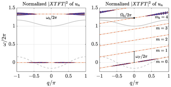
Figure 1. Plot of the $XTFT$ of exact breathers together with the dispersion relations for $u_n$ (continuous line) and $c_n$ (dashed line), the latter only for reference. (Left) Stationary soliton-breather. (Right) Moving soliton-breather, resonant lines and the breather line, $m_b=4$. The breather frequency in the moving frame ${\Omega }_b=m_b{\omega }_F$ and the fundamental frequency ${\omega }_F$ are also marked. In this case the step $s=1$. See Section 4 for details.

Exact traveling wave: 

An exact traveling wave with velocity $V_b$ is characterized by a function or sum of functions of the form:

$$u_n=f(n-V_{b}t,\Omega t),$$

with f a $2\pi$ periodic on its second one, and with the following condition below.

Fundamental time and step: 

There exist a fundamental time $T_F$ and an integer number called the step s, so the profile f repeats exactly after a time $T_F$. The velocity is then $V_b=s/T_F$.

Localized solutions: 

If f is localized in the first variable, it may be a breather, soliton, or kink. We will refer to it as a breather for simplicity. Then, we write the second variable as ${\Omega }_{b}t$. If it is delocalized, it is an exact extended traveling wave.

Fundamental frequency: 

${\omega }_F=2\pi /T_F$. The relevant frequencies are integer multiples of ${\omega }_F$, among which is the frequency associated to the velocity, i.e., the frequency at which a traveler in the moving frame encounters particles $2\pi V_b=s{\omega }_F$.

Frequency in the moving frame: 

$\Omega$ is the frequency in the moving frame, because if an observer moves with the breather, then $n-V_{b}t\approx 0$, and there remains a single frequency $\Omega$, ${\Omega }_b$ for the breather. We do not take into account the variation due to the discreteness.

Exactness: 

The exactness condition implies that $\Omega =m{\omega }_F$ for the integer m, or $m_b$ for the breather.

Harmonic modes: 

The breather, as any function of $(n,t)$, can be expressed as a sum of harmonic waves, also called modes $u_q=A_{q}exp\left(\mathrm{i}[qn-{\omega }_{q}t]\right)$, with ${\omega }_q$ being the laboratory frequency of each mode.

Resonant modes: 

Resonant modes with the breather are all the modes that advance the step s in the time $T_F$, that is, they are also exact with the same step and fundamental frequency. They can be written as $A_{q}exp\left(\mathrm{i}[(qn-V_{b}t)-m{\omega }_{F}t]\right)$.

Resonant lines: 

Therefore, the laboratory frequencies of the resonant modes are given by ${\omega }_q=m{\omega }_F+q{V}_b$. They form parallel straight lines called resonant lines, with slope $V_b$, and cross the vertical axis ($q=0$) at ${\Omega }_m=m{\omega }_F$, for the m integer. All modes in a resonant line travel with speed $V_b$ and have the same frequency in the moving frame ${\Omega }_m=m{\omega }_F$.

Breather line: 

All the modes in the spectrum of the localized exact solution $u_n$ are within one resonant line, with $m=m_b$, that is, the breather line. Note that the breather line ends at $q=\pi$ and reappears at $q=\pi -2\pi =-\pi$ as a different resonant line.

Breather frequency in the moving frame: 

The breather line crosses the vertical axis ($q=0$) at ${\Omega }_b=m_b{\omega }_F$, the frequency of the breather in the moving frame.

Transformation to the moving frame: 

Changing the frame of reference to the one moving with the breather, it is equivalent to the transformation $\omega \to {\omega }_{MF}=\omega -q{V}_b$. The resonant lines and the breather line become horizontal lines with the frequencies in the moving frame.

Soliton or kink: 

If ${\Omega }_b=0$, the excitation is a kink or soliton, that is, a static profile in the moving frame.

Wing: 

If a resonant line crosses the dispersion band, there is a resonant phonon, i.e., a solution to the linearized equation, that may bring about a wing. It is an extended wave that travels with the localized solution, becoming a pterobreather, pterosoliton, or pterokink. The wing may be an integral part of the solution to the nonlinear dynamical equations, that is, it will not exist without the wing [42].

Commensurability condition: 

The breather line frequency change for $\Delta q=2\pi$ is $\Delta {\Omega }_b=V_b\Delta q=2\pi V_b$, the velocity frequency, which is given by $s{\omega }_F$. Then,

$$\frac{{\Omega }_b}{\Delta {\Omega }_b}=\frac{{\Omega }_b}{2\pi V_b}=\frac{m_b}{s}$$

(17)

is a rational number. This important property allows for the determination of $m_b$, s, ${\omega }_F$, ${\Omega }_b$, and $V_b=\Delta {\Omega }_b/2\pi$, by simple inspection of the breather spectrum. $\Delta {\Omega }_b$ is also the difference in frequency between the breather line and its continuation when $\pi \to -\pi$. The moving frame frequency and the velocity frequency are commensurate.

5. Linear Approximations

In this section we obtain, the linearized equations corresponding to the dynamical Equations (8) and (9). We will use them to obtain the dispersion relations (DRs), also called the phonon bands, both for the variables $u_n$ and $c_n$, while there is no dispersion relation for ${\rho }_n={\left|c_n\right|}^2$. They provide the vibrational modes at small amplitude, the phonons, and they are necessary to understand the spectrum of larger-amplitude polarobreathers formed with modes that separate from the linear ones, as observed in Section 9 and Section 10. In general, the larger the amplitude, the larger the separation from the phonon band.

The dispersion relations are also useful for the tail analysis used in Section 6 and Section 7, which supposes that a localized nonlinear solution has a core of large amplitude that decreases at sites further away from the core, forming a tail of decreasing amplitude. A few sites away from the core, when the amplitude is small enough, the lattice variables would abide by the linear dispersion relations, with a decreasing exponential solution valid only to one side of the core and at some distance from it. This simple method is extremely useful for predicting the properties of nonlinear excitations, such as the increase or decrease in frequency with respect to phonons with the same wavenumber. In this way, the properties of the polarobreathers in Section 9 and Section 10 can be easily understood.

If we expand the terms in the dynamical Equations (8) and (9) to the first order in their variables, using ${\omega }_0^2=U^{″}\left(0\right)=4{\pi }^2$, $C=V^{″}\left(1\right)=72\epsilon =3.6$, and

$$\begin{array}{cc}\hfill J(u_{n+1}-u_n)=& J\left(0\right)+J^{\prime }\left(0\right)(u_{n+1}-u_n)+\dots =I_0-\alpha I_0(u_{n+1}-u_n)+\dots ,\hfill \\ \hfill J^{\prime }(u_{n+1}-u_n)=& J^{\prime }\left(0\right)+J^{″}\left(0\right)(u_{n+1}-u_n)+\dots =-\alpha I_0+{\alpha }^2{I}_0(u_{n+1}-u_n)+\dots ,\hfill \end{array}$$

and also seeing (6), we obtain:

$$\begin{array}{cc}\hfill {\ddot{u}}_n=& -{\omega }_0^2{u}_n-C(2u_n-u_{n+1}-u_{n-1})\hfill \\ \hfill & +\alpha I_0[1-\alpha (u_{n+1}-u_n)](c_n^{*}{c}_{n+1}+c_{n+1}^{*}{c}_n)\hfill \\ \hfill & -\alpha I_0[1-\alpha (u_n-u_{n-1})](c_{n-1}^{*}{c}_n+c_n^{*}{c}_{n-1}),\hfill \end{array}$$

(18)

$$\begin{array}{cc}\hfill \mathrm{i}\tau {\dot{c}}_n=& E_n{c}_n-I_0[1-\alpha (u_{n+1}-u_n)]c_{n+1}-I_0[1-\alpha (u_n-u_{n-1})]c_{n-1}.\hfill \end{array}$$

(19)

Keeping only the linear terms in (18) and (19), the lattice and the charge decouple, and we obtain a fully linearized system of equations:

$$\begin{array}{}(20)& \hfill {\ddot{u}}_n=& -{\omega }_0^2{u}_n-C\left(2u_n-u_{n+1}-u_{n-1}\right),\hfill (21)& \hfill \mathrm{i}\tau {\dot{c}}_n=& E_n{c}_n-I_0\left(c_{n+1}+c_{n-1}\right).\hfill \end{array}$$

The solutions of linear equations have an exponential form with imaginary exponents if they are bounded, that is, they have the form $u_n=exp\left(\mathrm{i}[qn-{\omega }_{L}t]\right)$ and $c_n=exp\left(\mathrm{i}[qn-{\omega }_{c}t]\right)$. The substitution of these expressions into the equations above leads to the dispersion relations:

$$\begin{array}{}(22)& \hfill {\omega }_L=& \pm {\left({\omega }_0^2+2C[1-cos\left(q\right)]\right)}^{1/2}=\pm {\left({\omega }_0^2+4C{sin}^2\left(\frac{q}{2}\right)\right)}^{1/2},\hfill (23)& \hfill {\omega }_c=& \frac{E_0}{\tau }-2\frac{I_0}{\tau }cos\left(q\right).\hfill \end{array}$$

We have included these dispersion relations in Figure 1 and in all $XTFT$ plots for reference. Note that the variables $u_n$ and $c_n$ become decoupled at the linear limit. Note also that wavenumbers $q=0$ and $q=\pm \pi$ correspond to stationary solutions. For $q=0$, the particles vibrate in phase with the same frequency, and for $q=\pm \pi$, they vibrate with an alternate pattern.

There could be some doubt about which variables the linearization should be performed in (18), because only the density matrix elements ${\rho }_{n,m}=c_n{c}_m^{*}$ appear. However, the linearization with respect to ${\rho }_{n,m}$ and $u_n$ results in the linear terms on ${\rho }_{n,m}$ becoming zero, and (8) does not change. There is no such problem for (19), as it is already linear in $c_n$ terms.

In Section 6 and Section 7, using the system of linearized Equations (20) and (21), we perform the tail analysis of stationary and moving localized excitations, respectively. We will compare the results in these sections with the present one.

6. Tail Analysis of Stationary Localized Excitations

For the tail of a stationary localized excitation, we propose the ansatz:

$$u_n=exp(-{\xi }_{L}n)exp\left(\mathrm{i}[qn-{\omega }_{L}t]\right),c_n=exp(-{\xi }_{c}n)exp\left(\mathrm{i}[qn-{\omega }_{c}t]\right),{\xi }_{L,c}\in {\mathbb{R}}_{+},$$

(24)

which is valid for $n>0$ (for $n<0$, we change the sign in front of n in the first exponentials). Note that both ${\xi }_{L,c}=0$ implies no localization and extended waves. With the ansatz (24) and assumption of the constant charge energy $E_n=E_0$, for all n, from the Equations (20) and (21) we obtain the following equations for the lattice and charge frequencies:

$$\begin{array}{}\mathrm{(25)}& \hfill {\omega }_L=& \pm {\left({\omega }_0^2+2C[1-cosh\left({\xi }_L\right)cos\left(q\right)]+\mathrm{i}2Csinh\left({\xi }_L\right)sin\left(q\right)\right)}^{1/2},\hfill \mathrm{(26)}& \hfill {\omega }_c=& \frac{E_0}{\tau }-2\frac{I_0}{\tau }\left[cosh\left({\xi }_c\right)cos\left(q\right)-\mathrm{i}sinh\left({\xi }_c\right)sin\left(q\right)\right],\hfill \end{array}$$

respectively, where q is the wavenumber. The momentum is given by $p_c=\overline{\tau }q$, with $\overline{\tau }=\tau /2\pi$ or ℏ in physical units. However, we will use both terms for q when there is no confusion, as they represent the same physical observable in different units.

If the frequencies ${\omega }_{L,c}$ are not real, that will imply decaying solutions; therefore, either both ${\xi }_{L,c}=0$, where we obtain extended solutions and the linear dispersion relations for the lattice and charge (22) and (23), or $sin\left(q\right)=0$, i.e., $q=0$ or $\pm \pi$, and for $q=0$ from (25) and (26), we obtain:

$$\begin{array}{c}\hfill \begin{array}{cc}\hfill {\omega }_L=& \pm {\left({\omega }_0^2+2C[1-cosh\left({\xi }_L\right)]\right)}^{1/2}\mathrm{with}\left|{\omega }_L\right|<{\omega }_0,\hfill \\ \hfill {\omega }_c=& \frac{E_0}{\tau }-2\frac{I_0}{\tau }cosh\left({\xi }_c\right)<\frac{E_0}{\tau }-2\frac{I_0}{\tau }.\hfill \end{array}\end{array}$$

(27)

From (27), it can be seen that the localization drives the frequencies below the linear spectrum (above for negative ${\omega }_L$), and further away the larger the localization is.

For $q=\pm \pi$, there is the opposite effect, i.e., localization increases the frequencies above the linear spectrum (below for negative ${\omega }_L$). From (25) and (26):

$$\begin{array}{c}\hfill \begin{array}{cc}\hfill {\omega }_L=& \pm {\left({\omega }_0^2+2C[1+cosh\left({\xi }_L\right)]\right)}^{1/2}\mathrm{with}\left|{\omega }_L\right|>{\left({\omega }_0^2+4C\right)}^{1/2},\hfill \\ \hfill {\omega }_c=& \frac{E_0}{\tau }+2\frac{I_0}{\tau }cosh\left({\xi }_c\right)>\frac{E_0}{\tau }+2\frac{I_0}{\tau }.\hfill \end{array}\end{array}$$

(28)

Note that the localization parameters ${\xi }_{L,c}$ do not need to be the same in (25) and (26) and (27) and (28) for the lattice and the charge. A good estimate would be $2{\xi }_c={\xi }_L$, as in the lattice Equation (8), the charge amplitude $c_n$ products $c_n{c}_{n\pm 1}^{*}$ appear. Furthermore,

$$c_n=exp(-{\xi }_{c}n)exp\left(\mathrm{i}[\pm \pi n-{\omega }_{c}t]\right)={(-1)}^{n}exp(-{\xi }_{c}n)exp(-\mathrm{i}{\omega }_{c}t)$$

has the same pattern as

$$c_n=exp(-{\xi }_{c}n)exp\left(\mathrm{i}[\pm \pi n+{\omega }_{c}t]\right)={(-1)}^{n}exp(-{\xi }_{c}n)exp\left(\mathrm{i}{\omega }_{c}t\right).$$

As the $\pm \pi$ modes are not actually traveling, the two modes will appear mixed, i.e.,

$$c_n(\pm \pi )=Aexp(-{\xi }_{c}n){(-1)}^{n}exp(-\mathrm{i}{\omega }_{c}t)+Bexp(-{\xi }_{c}n){(-1)}^{n}exp\left(\mathrm{i}{\omega }_{c}t\right),$$

and

$$c_n^{*}(\pm \pi )=A^{*}exp(-{\xi }_{c}n){(-1)}^{n}exp\left(\mathrm{i}{\omega }_{c}t\right)+B^{*}exp(-{\xi }_{c}n){(-1)}^{n}exp(-\mathrm{i}{\omega }_{c}t),$$

where $A,B\in \mathbb{C}$. In this way, we can obtain the time dependence on the charge probability ${\rho }_n={\left|c_n\right|}^2$, i.e.,

$${\rho }_n=exp(-2{\xi }_{c}n)\left({\left|A\right|}^2+{\left|B\right|}^2+A{B}^{*}exp(-2\mathrm{i}{\omega }_{c}t)+A^{*}Bexp\left(2\mathrm{i}{\omega }_{c}t\right)\right).$$

If we write $A{B}^{*}=\left|A\right|\left|B\right|exp\left(\mathrm{i}\delta \right)$ for $\delta =arg\left(A\right)-arg\left(B\right)$, we obtain:

$$\begin{array}{cc}\hfill {\rho }_n=& exp(-2{\xi }_{c}n)\left({\left|A\right|}^2+{\left|B\right|}^2+2\left|A\right|\left|B\right|cos(2{\omega }_{c}t-\delta )\right)\hfill \\ \hfill =& {\left(\right|A|}^2+{\left|B\right|}^2)exp(-2{\xi }_{c}n)+2\left|A\right|\left|B\right|exp(-2{\xi }_{c}n)cos(2{\omega }_{c}t-\delta ).\hfill \end{array}$$

In this way, we will observe in the charge probability spectrum two frequencies: ${\omega }_{\rho }=0$, corresponding to a stationary deformation, and ${\omega }_{\rho }=4\frac{I_0}{\tau }cosh\left({\xi }_c\right)$, where the charge probability spectrum is independent of the $E_0$ value. Note that as $|c_n{|}^2$ is an observable, its frequencies can be measured; from them, we can deduce the difference in frequencies from the $q=\pi$ and $q=0$ modes of $c_n$, but not their actual value, because there are no physical means of knowing which is the shift $E_0/\tau$ of the $c_n$ frequencies. We choose for our convenience the value of $E_0$ that makes $c_n$ periodic with a commensurate period with the lattice one. However, that selection has no physical consequences, and we will plot the $c_n$ spectrum corresponding to $E_0=0$ for simplicity.

7. Tail Analysis of Moving Localized Excitations

We can repeat the tail analysis above for the moving solutions. In this case, the trial solutions in (24) are changed to:

$$\begin{array}{cc}\hfill u_n=& exp(-{\xi }_L[n-V_{b}t])exp\left(\mathrm{i}(q[n-V_{b}t]-{\Omega }_{L}t)\right),\hfill \end{array}$$

(29)

$$\begin{array}{cc}\hfill c_n=& exp(-{\xi }_c[n-V_{b}t])exp\left(\mathrm{i}(q[n-V_{b}t]-{\Omega }_{c}t)\right).\hfill \end{array}$$

(30)

These ansätze are valid for $n>V_{b}t$ or for $n<V_{b}t$ changing ${\xi }_{L,c}\in {\mathbb{R}}_{+}$ to $-{\xi }_{L,c}$. Considering first the ansatz (29) for $u_n$, in the moving frame $n=V_{b}t$, the frequency is ${\Omega }_L$, with

$$u_{n+1}=exp(-{\xi }_L)exp\left(\mathrm{i}q\right)u_n,$$

that is, $u_{n+1}$ is vibrating with the same frequency ${\Omega }_L$ but with a smaller amplitude and a difference of phase q. The general solution for a traveling breather would be a sum of terms as $u_n$ in (29), with the same frequency ${\Omega }_L$ in the moving frame. The parameter ${\xi }_L$ would be also dependent on each mode. The larger ${\xi }_L$ is, the more localized the specific localized mode would be, and likewise for $c_n$ with the ansatz (30).

We also assume that the general solution is exact, that is, it repeats after some fundamental time $T_F$ displaced an integer number of sites $s=V_b{T}_F$, called the step. Then, all the modes (29) have the same properties, that is, $V_b$, $T_F$, and step s. The fundamental frequency is defined as ${\omega }_F=2\pi /T_F$. The exactness condition implies that ${\Omega }_L=m_L{\omega }_F$ for the integers $m_L$ and $V_b=s({\omega }_F/2\pi )$. See Ref. [25] for more details. The fundamental period $T_F$ could, in principle, be different for the lattice and the charge amplitude, but for the common system to be exact, there should be integer multiples of both periods to obtain a common fundamental period $T_F$ and step s.

Substituting the ansatz (29) for $u_n$ into the linear Equation (20), we obtain:

$${\left([q{V}_b+{\Omega }_L]+\mathrm{i}{\xi }_L{V}_b\right)}^2={\omega }_0^2+2C[1-cosh\left({\xi }_L\right)cos\left(q\right)]+\mathrm{i}2Csinh\left({\xi }_L\right)sin\left(q\right).$$

(31)

Compare (31) with Equation (25) of Section 6. Expanding the left hand side of (31), we arrive at two equations for the real and imaginary part:

$$\begin{array}{c}\hfill \begin{array}{cc}\hfill {\omega }_L^2=& {\xi }_L^2{V}_b^2+{\omega }_0^2+2C[1-cosh\left({\xi }_L\right)cos\left(q\right)],\hfill \\ \hfill {\xi }_L{V}_b{\omega }_L=& Csinh\left({\xi }_L\right)sin\left(q\right).\hfill \end{array}\end{array}$$

(32)

For compactness, we use the laboratory frequency:

$${\omega }_L=q{V}_b+{\Omega }_L=q{V}_b+m_L{\omega }_F,$$

of the moving mode with wavenumber q.

For delocalized waves, with ${\xi }_L=0$, from (32), we recover the lattice dispersion relation (22) and the group velocity of the linear extended waves:

$$\begin{array}{cccc}\hfill {\omega }_L^2=& {\omega }_0^2+2C[1-cos\left(q\right)],\hfill & & \mathrm{for} {\xi }_c=0,\hfill \\ \hfill V_b=& \frac{Csin\left(q\right)}{{\omega }_L},\mathrm{equal}\mathrm{to}\frac{\partial {\omega }_L}{\partial q},\hfill & & \mathrm{for} {\xi }_c=0.\hfill \end{array}$$

The latter equation indicates that there is only one mode with a given $V_b$: the one where the slope of the dispersion relation is precisely $V_b$. This is why it is not possible to have a coherent wave at the linear limit, as every mode has a different velocity.

As $cosh\left({\xi }_L\right)\ge 1$ and increases with the localization parameter ${\xi }_L$, in addition, if $\pi /2<\left|q\right|<\pi$, $cos\left(q\right)<0$, and if $0<\left|q\right|<\pi /2$, $cos\left(q\right)>0$, then from the first equation of (32), we find that

$$\begin{array}{cccc}\hfill {\omega }_L{\left({\xi }_L\right)}^2-{\omega }_L{\left(0\right)}^2=& {\xi }_L^2{V}_b^2+4C|cos\left(q\right)|{sinh}^2\left(\frac{{\xi }_L}{2}\right),\hfill & & \mathrm{for} \frac{\pi }{2}\le \left|q\right|\le \pi ,\hfill \\ \hfill {\omega }_L{\left({\xi }_L\right)}^2-{\omega }_L{\left(0\right)}^2=& {\xi }_L^2{V}_b^2-4C|cos\left(q\right)|{sinh}^2\left(\frac{{\xi }_L}{2}\right),\hfill & & \mathrm{for} 0\le \left|q\right|<\frac{\pi }{2}.\hfill \end{array}$$

Therefore, it can be seen that ${\omega }_c^2$ is above the linear frequency for the same $\left|q\right|\in [\pi /2,\pi ]$. However, when $\left|q\right|$ becomes smaller than $\pi /2$, the two terms of the nonlinear correction have different signs, but they are also clearly above the linear frequency in a close proximity to $\left|q\right|=\pi /2$, at which point the negative term is zero. The main conclusion is that a solution such as the one proposed is possible below the linear spectrum, closer to $q=0$, and above the linear spectrum, closer to $\left|q\right|=\pi$. The latter would be the case for our system.

Let us analyze the ansatz for $c_n$, given by (30). The substitution into Equation (21) with the constant $E_n=E_0$ leads to the following equation:

$$\tau {\omega }_c+\mathrm{i}\tau {\xi }_c{V}_b=E_0-2I_0\left[cosh\left({\xi }_c\right)cos\left(q\right)-\mathrm{i}sinh\left({\xi }_c\right)sin\left(q\right)\right],$$

(33)

where the charge amplitude laboratory frequency is given by:

$${\omega }_c=q{V}_b+{\Omega }_c=q{V}_b+m_c{\omega }_F.$$

For the comparison with the stationary case, compare Equation (33) with (26) of the previous section.

Equation (33) leads to two equations for the real and imaginary part:

$$\begin{array}{cc}\hfill E_c=& \tau {\omega }_c=E_0-2I_{0}cos\left(q\right)cosh\left({\xi }_c\right),\hfill \\ \hfill V_b=& 2\frac{I_0}{\tau }sin\left(q\right)\frac{sinh\left({\xi }_c\right)}{{\xi }_c}.\hfill \end{array}$$

The first equation gives the energy of the system, and the second gives the velocity. Note that a change in frequency ${\tilde{\omega }}_c-E_o/\tau$, corresponding to ${\tilde{c}}_n=c_{n}exp(\mathrm{i}{E}_0/\tau )$, is the frequency with the corresponding energy ${\tilde{E}}_c=\tau {\tilde{\omega }}_c-E_0$ for the system with ${\tilde{E}}_0=0$.

For ${\xi }_c=0$, we recover the linear dispersion relation (23) together with the group velocity:

$$\begin{array}{cccc}\hfill E_c=& \tau {\omega }_c=E_0-2I_{0}cos\left(q\right),\hfill & & \mathrm{for} {\xi }_c=0,\hfill \\ \hfill V_b=& 2\frac{I_0}{\tau }sin\left(q\right),\mathrm{equal}\mathrm{to}{V}_b=\frac{\partial {\omega }_c}{\partial q},\hfill & & \mathrm{for} {\xi }_c=0.\hfill \end{array}$$

Again, there is only one linear mode for a given velocity $V_b$, and coherent wave packages of $c_n$ are not possible at the linear limit or close to it.

The modes with a higher localization ${\xi }_c$ value correspond to faster propagating modes compared to the corresponding linear ones, since $sinh\left({\xi }_c\right)/{\xi }_c>1$ for $|{\xi }_c|>0$. From the equivalent considerations above, for $\left|q\right|\in [\pi /2,\pi ]$, the localization energies $E_c\left({\xi }_c\right)$ are above the linear energies $E_c\left(0\right)$, and vice versa for $0\le \left|q\right|<\pi /2$, i.e.,

$$\begin{array}{cccc}\hfill E_c\left({\xi }_c\right)-E_c\left(0\right)=& 4I_0|cos\left(q\right)|{sinh}^2\left(\frac{{\xi }_c}{2}\right)>0,\hfill & & \mathrm{for} \frac{\pi }{2}\le \left|q\right|\le \pi ,\hfill \\ \hfill E_e\left({\xi }_c\right)-E_c\left(0\right)=& -4I_0|cos\left(q\right)|{sinh}^2\left(\frac{{\xi }_c}{2}\right)<0,\hfill & & \mathrm{for} 0\le \left|q\right|<\frac{\pi }{2}.\hfill \end{array}$$

8. Numerical Methods

In this section, we describe numerical methods used to solve the canonical Hamiltonian system (11)–(14) and obtain numerically exact polarobreather solutions.

8.1. Numerical Integration of the Canonical Hamiltonian Equations

To solve the canonical Hamiltonian Equations (11)–(14) numerically, we consider the exact charge probability (4) conserving, second-order semi-implicit splitting method $\mathrm{P}\mathrm{Q}\mathrm{D}\mathrm{W}\mathrm{D}\mathrm{Q}\mathrm{P}$ from the recently proposed splitting method class specifically developed for the semiclassical Hamiltonian dynamics of charge transfer in nonlinear lattices [33]. The symmetric and symplecticity-preserving method $\mathrm{P}\mathrm{Q}\mathrm{D}\mathrm{W}\mathrm{D}\mathrm{Q}\mathrm{P}$ is constructed by splitting the total Hamiltonian (10) in the sum of the following Hamiltonians: $H=H_{\mathrm{Q}}+H_{\mathrm{P}}+H_{\mathrm{D}}+H_{\mathrm{W}}$, where

$$\begin{array}{}\mathrm{(34)}& \hfill H_{\mathrm{Q}}& =\frac{1}{2}\sum _{n=1}^N{p}_n^2,\hfill \mathrm{(35)}& \hfill H_{\mathrm{P}}& =\sum _{n=1}^N\left[U\left(u_n\right)+V(1+u_{n+1}-u_n)\right],\hfill \mathrm{(36)}& \hfill H_{\mathrm{D}}& =\frac{1}{2\tau }\sum _{n=1}^N{E}_n\left(a_n^2+b_n^2\right),\hfill \mathrm{(37)}& \hfill H_{\mathrm{W}}& =-\frac{1}{\tau }\sum _{n=1}^{N}J(u_{n+1}-u_n)\left(a_n{a}_{n+1}+b_n{b}_{n+1}\right).\hfill \end{array}$$

Importantly, corresponding Hamiltonian systems associated to each Hamiltonian (34)–(36) can be solved exactly, and solutions are identified with the analytic symplectic flows ${\varphi }_t^{\mathrm{Q}}$, ${\varphi }_t^{\mathrm{P}}$, and ${\varphi }_t^{\mathrm{D}}$, respectively. Meanwhile, we solve the Hamiltonian system of (37) with the symplectic implicit midpoint rule, whose solution we identify with the flow map ${\psi }_h^{\mathrm{W}}$, where $h>0$ is the time step. Thus, the numerical method $\mathrm{P}\mathrm{Q}\mathrm{D}\mathrm{W}\mathrm{D}\mathrm{Q}\mathrm{P}$ with the flow map ${\psi }_h$ is a symmetric composition of flows ${\varphi }_t^{\mathrm{Q}}$, ${\varphi }_t^{\mathrm{P}}$, and ${\varphi }_t^{\mathrm{D}}$ as well as the flow map ${\psi }_h^{\mathrm{W}}$, i.e.,

$${\psi }_h={\varphi }_{h/2}^{\mathrm{P}}\circ {\varphi }_{h/2}^{\mathrm{Q}}\circ {\varphi }_{h/2}^{\mathrm{D}}\circ {\psi }_h^{\mathrm{W}}\circ {\varphi }_{h/2}^{\mathrm{D}}\circ {\varphi }_{h/2}^{\mathrm{Q}}\circ {\varphi }_{h/2}^{\mathrm{P}},$$

where the symmetry of the method follows from the construction, symplecticity follows from the composition of symplectic maps, and the charge probability conservation (4) follows from the implicit midpoint step ${\psi }_h^{\mathrm{W}}$, which preserves quadratic invariants [43].

Advancing from state $(u_n,a_n,p_n,b_n)$ to a new state $(U_n,A_n,P_n,B_n)$ after one time step h for all $n=1,\dots ,N$, the solution given by the flow ${\varphi }_h^{\mathrm{Q}}$ of the Hamiltonian system associated with the split dynamics (34) reads:

$$U_n=u_n+h{p}_n,A_n=a_n,P_n=p_n,B_n=b_n.$$

Similarly, the solution given by the flow ${\varphi }_h^{\mathrm{P}}$ of the Hamiltonian system associated with the split dynamics (35) reads:

$$\begin{array}{cc}\hfill U_n=& u_n,\hfill \\ \hfill A_n=& a_n,\hfill \\ \hfill P_n=& p_n-h\left[U^{\prime }\left(u_n\right)-V^{\prime }(1+u_{n+1}-u_n)+V^{\prime }(1+u_n-u_{n-1})\right],\hfill \\ \hfill B_n=& b_n.\hfill \end{array}$$

Notice that during the applications of the flow maps ${\varphi }_h^{\mathrm{Q}}$ and ${\varphi }_h^{\mathrm{P}}$, only the lattice variables $u_n$ and $p_n$ get updated, while the charge variables $a_n$ and $b_n$ remain unchanged.

To find the exact expression of the flow ${\varphi }_h^{\mathrm{D}}$ of the Hamiltonian system associated with the Hamiltonian (36), we state the associated system of differential equations:

$$\begin{array}{}\mathrm{(38)}& \hfill {\dot{u}}_n& =0,\hfill \mathrm{(39)}& \hfill {\dot{a}}_n& =\frac{1}{\tau }{E}_n{b}_n,\hfill \mathrm{(40)}& \hfill {\dot{p}}_n& =0,\hfill \mathrm{(41)}& \hfill {\dot{b}}_n& =-\frac{1}{\tau }{E}_n{a}_n,\hfill \end{array}$$

where $n=1,\dots ,N$. From (38)–(41), it is easy to see that we obtain decoupled harmonic oscillator Equations (39) and (41) for the variables $a_n$ and $b_n$, which can be solved exactly for all n and any initial condition $(a_n^0,b_n^0)$, i.e.,

$$\begin{array}{cc}\hfill a_n\left(t\right)& =a_n^{0}cos\left({\omega }_{n}t\right)+b_n^{0}sin\left({\omega }_{n}t\right),\hfill \\ \hfill b_n\left(t\right)& =-a_n^{0}sin\left({\omega }_{n}t\right)+b_n^{0}cos\left({\omega }_{n}t\right),\hfill \end{array}$$

where ${\omega }_n={\tau }^{-1}{E}_n$. Thus, the exact (explicit) solution given by the flow ${\varphi }_h^{\mathrm{D}}$ of the Hamiltonian system (38)–(41) is in the following form:

$$\begin{array}{cc}\hfill U_n=& u_n,\hfill \\ \hfill A_n=& a_{n}cos\left({\omega }_{n}h\right)+b_{n}sin\left({\omega }_{n}h\right),\hfill \\ \hfill P_n=& p_n,\hfill \\ \hfill B_n=& -a_{n}sin\left({\omega }_{n}h\right)+b_{n}cos\left({\omega }_{n}h\right).\hfill \end{array}$$

If all $E_n=0$, then the flow map ${\varphi }_h^{\mathrm{D}}$ is just an identity map.

We conclude this section by listing the explicit representation in the component form of the implicit midpoint map ${\varphi }_h^{\mathrm{W}}$:

$$\begin{array}{}\mathrm{(42)}& \hfill U_n& =u_n,\hfill \mathrm{(43)}& \hfill A_n& =a_n-\frac{h}{\tau }\left(J(u_{n+1}-u_n)\frac{B_{n+1}+b_{n+1}}{2}+J(u_n-u_{n-1})\frac{B_{n-1}+b_{n-1}}{2}\right),\hfill \mathrm{(44)}& \hfill P_n& =p_n-\frac{h}{\tau }\left(J^{\prime }(u_{n+1}-u_n){\zeta }_{n,n+1}-J^{\prime }(u_n-u_{n-1}){\zeta }_{n,n-1}\right),\hfill \mathrm{(45)}& \hfill B_n& =b_n+\frac{h}{\tau }\left(J(u_{n+1}-u_n)\frac{A_{n+1}+a_{n+1}}{2}+J(u_n-u_{n-1})\frac{A_{n-1}+a_{n-1}}{2}\right),\hfill \end{array}$$

where

$${\zeta }_{n,n^{\prime }}=\frac{1}{4}\left[(A_n+a_n)(A_{n^{\prime }}+a_{n^{\prime }})+(B_n+b_n)(B_{n^{\prime }}+b_{n^{\prime }})\right]$$

and the momentum value $P_n$ in (44) gets updated after the linear system of Equations (43) and (45), formed from all $n=1,\dots ,N$, solved for the charge variables $A_n$ and $B_n$. In what follows, all numerical results are obtained with $N=64$ and $h=0.01$.

The authors of [33] also proposed fully explicit structure-preserving splitting methods for the semiclassical Hamiltonian dynamics of charge transfer in nonlinear lattices. While the explicit methods are computationally more efficient compared to the semi-implicit splitting method $\mathrm{P}\mathrm{Q}\mathrm{D}\mathrm{W}\mathrm{D}\mathrm{Q}\mathrm{P}$, they do not exactly conserve charge probability (4), which is essential for obtaining numerically exact polarobreather solutions. Since numerically exact polarobreather solutions are determined for the discrete dynamical system given by the numerical method $\mathrm{P}\mathrm{Q}\mathrm{D}\mathrm{W}\mathrm{D}\mathrm{Q}\mathrm{P}$ with the time step h, the prospect for future research is to extend proposed structure-preserving splitting methods in [33] to computationally efficient higher-order methods [44] for the computation of exact polarobreather solutions in crystal lattice models with realistic potentials [25].

8.2. Numerical Algorithm for Computation of Exact Polarobreathers

The numerical integration method $\mathrm{P}\mathrm{Q}\mathrm{D}\mathrm{W}\mathrm{D}\mathrm{Q}\mathrm{P}$ described above provides a good means to obtain numerical solutions to (11)–(14) at discrete time instances for arbitrary initial conditions, which are prescribed in Section 9 and Section 10. Thus, we can obtain approximate stationary and moving polarobreather solutions with exact charge probability conservation (4) and approximate energy conservation in long-time simulations using the symplectic integrator [43]. For examples, see Section 9.1 and Section 10.1.

The obtained approximate solutions can be used as initial guess solutions for the numerical algorithm presented below to compute numerically exact polarobreather solutions; see Section 9.2 and Section 10.2. The developed algorithm is based on the Gauss–Newton algorithm for nonlinear least squares [45] with constraints:

$$\underset{x,E_0,\lambda }{min}F(x;E_0)+g{\left(x\right)}^T\lambda ,$$

(46)

with the objective function:

$$F(x;E_0)=\frac{1}{2}f{(x;E_0)}^{T}f(x;E_0),$$

where

$$x\left(t\right)={\left(u_1\left(t\right),\dots ,u_N\left(t\right),a_1\left(t\right),\dots ,a_N\left(t\right),p_1\left(t\right),\dots ,p_N\left(t\right),b_1\left(t\right),\dots ,b_N\left(t\right)\right)}^T\in {\mathbb{R}}^{4N}$$

is the solution vector of (11)–(14) at time t with $E_n=E_0$, and $\lambda \in {\mathbb{R}}^M$ is a vector of Lagrange multipliers for M number of constraints; see below (48). $M=N+2$ and $M=2$ for the stationary and moving exact polarobreather calculations, respectively. In addition, we define shift operator ${\mathcal{S}}_s$ acting on the components of vector $x\left(t\right)$, such that

$${\left({\mathcal{S}}_{s}x\left(t\right)\right)}_n=x_{n+s}\left(t\right),$$

taking into account the periodic boundary conditions. Then,

$$f(x;E_0)={\mathcal{S}}_{s}x\left(T_F\right)-x\left(0\right),$$

(47)

where $x\left(T_F\right)$ is the numerical solution of (11)–(14) at time $T_F$ obtained with exact charge probability (4) conserving the splitting method $\mathrm{P}\mathrm{Q}\mathrm{D}\mathrm{W}\mathrm{D}\mathrm{Q}\mathrm{P}$ and time step h of Section 8.1.

We recall that $T_F$ is the fundamental period and the step $s=0$ for the stationary polarobreathers, while $s>0$ if the traveling polarobreather moves to the right and $s<0$ if the traveling polarobreather moves to the left. Note that the objective function in (46) is minimized for x, Lagrange multipliers $\lambda$, and the constant charge shift energy value $E_0$ (parameter value in the system) with the fixed value of $T_F$ and s, which are estimated from the approximate solution spectra; see Section 9 and Section 10.

The vector function $g\left(x\right)\in {\mathbb{R}}^M$ contains imposed constraints such as the charge probability (4) conservation, without the loss of generality $b_N=0$, to eliminate the charge rotational invariance by an arbitrary angle $\theta$, i.e., canonical Hamiltonian Equations (11)–(14) are invariant under the transformation ${\overline{c}}_n=c_{n}exp\left(\mathrm{i}\theta \right)$. Thus,

$$g\left(x\right)=\left[\begin{array}{c}{\displaystyle \sum _{n=1}^N\left(a_n^2+b_n^2\right)-2\tau }\\ b_N\end{array}\right].$$

(48)

For the computation of exact stationary polarobreathers, we also impose, in addition to (48), that all $p_n=0$, which leads to time-periodic stationary polarobreather solutions $p_n\left(T_F\right)=p_n\left(0\right)=0$. The quadratic constraint in (48) demonstrates the necessity for the exact charge probability (4), conserving numerical methods, e.g., the use of $\mathrm{P}\mathrm{Q}\mathrm{D}\mathrm{W}\mathrm{D}\mathrm{Q}\mathrm{P}$.

We consider the damped Gauss–Newton algorithm to solve the optimization problem (46), i.e., (46) is reduced to the regularized linear least squares:

$$\begin{array}{c}\hfill \underset{\Delta x,\Delta E_0,\lambda }{min}\frac{1}{2}{\left(f(x^k;E_0^k)+J(x^k,E_0^k)\left[\begin{array}{c}\Delta x\\ \Delta E_0\end{array}\right]\right)}^T\left(f(x^k;E_0^k)+J(x^k,E_0^k)\left[\begin{array}{c}\Delta x\\ \Delta E_0\end{array}\right]\right)\\ \hfill +{\left(g\left(x^k\right)+G\left(x^k\right)\Delta x\right)}^T\lambda +\frac{1}{2}\mu \left(\Delta x^T\Delta x+{\Delta E_0}^2\right),\end{array}$$

(49)

where $\mu \ge 0$ is the regularization parameter adjusted with each iteration, and k is the iteration index, where $k=0,1,2,\dots$, $x^k$, and $E_0^k$ are the solution and energy $E_0$ value at the k-th iteration, respectively. $J(x^k,E_0^k)\in {\mathbb{R}}^{4N\times 4N+1}$ is the Jacobian matrix of (47), while $G\left(x^k\right)\in {\mathbb{R}}^{M\times 4N}$ is the Jacobian matrix of the constraint vector function $g\left(x\right)$. The Jacobian matrix $G\left(x^k\right)$ can easily be evaluated analytically. However, in theory, the Jacobian matrix $J(x^k,E_0^k)$ can also be evaluated analytically but with high difficulty. Thus, we evaluate it numerically. Accordingly, increments (descent directions) $\Delta x\in {\mathbb{R}}^{4N}$ and $\Delta E_0\in \mathbb{R}$.

The minimum of the linear least squares (49) is the solution to the following linear system of equations:

where I and 0 are identity and zero matrices of appropriate dimensions, and

$$x^{k+1}=x^k+\Delta x,E_0^{k+1}=E_0^k+\Delta E_0.$$

We set the stopping criteria on the maximal absolute errors of functions $f(x;E_0)$ and $g\left(x\right)$ with tolerance ${10}^{-14}$. Thus, the converged solution satisfies (pointwise) time periodicity $T_F$ and the step s conditions (47), as well as the system constraints $g\left(x\right)$, to high numerical accuracy, which are then preserved by the numerical method $\mathrm{P}\mathrm{Q}\mathrm{D}\mathrm{W}\mathrm{D}\mathrm{Q}\mathrm{P}$ to perform spectral analysis.

For all $\mu >0$, $x^k$, and $E_0^k$, the matrix $J{(x^k,E_0^k)}^{T}J(x^k,E_0^k)+\mu I_{4N+1,4N+1}$ is positive definite. If ${\sum }_{n=1}^N{\left(a_n^k\right)}^2+{\left(b_n^k\right)}^2>0$ with $b_N^k=0$, then the Jacobian matrix $G\left(x^k\right)$ has a full row rank and the linear system above has a unique solution such that ${\sum }_{n=1}^N{\left(a_n^{k+1}\right)}^2+{\left(b_n^{k+1}\right)}^2>0$ and $b_N^{k+1}=0$, which implies that the Jacobian matrix $G\left(x^{k+1}\right)$ has a full row rank and the linear system has a unique solution with $x^{k+1}$ and $E_0^{k+1}$. To verify this, assume the opposite: ${\sum }_{n=1}^N{\left(a_n^{k+1}\right)}^2+{\left(b_n^{k+1}\right)}^2=0$. This implies that $a_n^{k+1}=b_n^{k+1}=0$ for all n, i.e., increments $\Delta a_n=-a_n^k$ and $\Delta b_n=-b_n^k$. From the unique solvability of the linear equations with $x^k$ and $E_0^k$, from the linear equations, we obtain:

$$\begin{array}{cc}\hfill 2\sum _{n=1}^N\left(\Delta a_n{a}_n^k+\Delta b_n{b}_n^k\right)& =-\sum _{n=1}^N\left({\left(a_n^k\right)}^2+{\left(b_n^k\right)}^2\right)+2\tau ,\hfill \\ \hfill -2\sum _{n=1}^N\left(a_n^k{a}_n^k+b_n^k{b}_n^k\right)& =-\sum _{n=1}^N\left({\left(a_n^k\right)}^2+{\left(b_n^k\right)}^2\right)+2\tau ,\hfill \\ \hfill \sum _{n=1}^N{\left(a_n^k\right)}^2+{\left(b_n^k\right)}^2& =-2\tau ,\hfill \end{array}$$

which yields a contradiction, since $\tau >0$. Thus, the linear system has a unique solution for all $x^k$ and $E_0^k$ if $x^0$ satisfies all constraints.

To update the regularization parameter $\mu$ after each iteration step in (49), we compute the gain ratio value:

$$\upsilon =2\left(F(x^k;E_0^k)-F(x^{k+1};E_0^{k+1})\right)/{\left[\begin{array}{c}\Delta x\\ \Delta E_0\end{array}\right]}^T\left(\mu \left[\begin{array}{c}\Delta x\\ \Delta E_0\end{array}\right]-J{(x^k,E_0^k)}^{T}f(x^k;E_0^k)\right).$$

The gain ratio value $\upsilon$ allows us to adjust the value of $\mu$ such that it decreases as we approach the minimum of the nonlinear least squares (46). We were able to obtain satisfactory convergence results; the numerical results demonstrated superlinear convergence if good starting $x^0$ and $E_0^0$ values are provided, with the update strategy for $\mu$, that is, double the value of $\mu$, if $\upsilon <0.25$, remaining the same value for the next iteration, unless $\upsilon >0.75$, then a three-times smaller value of $\mu$ is considered. As an initial value, we chose $\mu ={10}^{-6}max\left[\mathrm{diag}\left(J{(x^0,E_0^0)}^{T}J(x^0,E_0^0)\right)\right]$.

9. Stationary Polarobreathers

9.1. Generation of Approximate Stationary Polarobreathers

The methods used to produce polarobreathers in this model (solving (11)–(14)) are extremely efficient; they have been used in previous works in one and two dimensions [33,38,39]. In this section, we present the method for the stationary case; the moving polarobreather case will be presented in the following Section 10.

We introduce nonzero initial conditions only for the velocities or momenta:

$${(p_{n^{*}-1},p_{n^{*}},p_{n^{*}+1},p_{n^{*}+2})}^T=\gamma {(-1,2,-2,1)}^T,\gamma \in {\mathbb{R}}_{\ne 0}.$$

(50)

The parameter $\gamma$ is related with the kinetic energy delivered to the system as $K_E=5{\gamma }^2$. The reference index $n^{*}$ can be arbitrary because the system is periodic, but we usually take $n^{*}=N/2$, for visual plotting purposes. The charge wave function is located initially with probability one, with the pattern:

$${(a_{n^{*}},b_{n^{*}})}^T=\sqrt{\tau }{(1,-1)}^T.$$

(51)

That is, the charge is completely localized at $n^{*}$ with probability one. This combined pattern (50) and (51) proves to be very efficient in obtaining quite good stationary solutions with long life. Other methods and patterns have also been investigated, for example, producing a local compression, which often brings about a stationary breather and two traveling ones in opposite directions. Moreover, different patterns for the positions and momenta have been considered. Many of them work quite well, but this is the preferred one for simplicity and for obtaining results. We describe the results for $\gamma =0.4$, corresponding to the kinetic energy $K_E=0.8$, in scaled units. Other values of $\gamma$ bring about qualitatively similar results.

We perform the 2D discrete Fourier transform in positions and time ($XTFT$) of time-series data on the variables $u_n$, $|c_n{|}^2$, and $c_n$, which are represented in Figure 2-top. For reference, the dispersion relations (22) and (23) for $u_n$ and $c_n$ are also plotted with gray solid and dashed lines, respectively. Numerical results were obtained, setting all $E_n=0$ in (11)–(14).

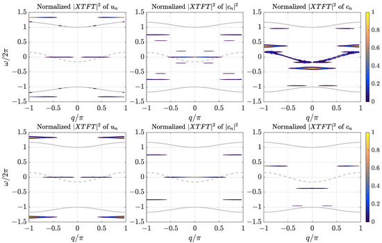
Figure 2. $XTFT$ of the lattice variables $u_n$, charge probability $|c_n{|}^2$, and probability amplitude $c_n$. (Top) Inexact stationary breather generated with $\gamma =0.4$ and kinetic energy $K_E=0.8$. (Bottom) Exact stationary breather obtained using the approximate polarobreather as an initial seed. See text.

As the first two quantities are real, for the $XTFT$ components, it holds that $F(-q,-\omega )$$=F^{*}(q,\omega )$ and $\left|F\right(-q,-\omega \left)\right|=\left|F\right(q,\omega \left)\right|$, which is a symmetry that can be observed in the corresponding two upper plots. Usually, in this case, the negative frequencies are not represented, but here, they are included for comparison with the $XTFT$ of $c_n$, where the symmetry does not hold, as $c_n$ is complex. Some main features from the top plots of Figure 2 can be discerned:

• For the $XTFT$ of $u_n$, there appear two horizontal lines at $\omega =0$, centered around $q=0$, and some frequency ${\omega }_L/2\pi \simeq 1.33$ above the dispersion relation and centered around $q=\pm \pi$. This means that the $u_n$ breather is composed of a soliton, that is, a static deformation with a displacement largely in phase and a staggered vibration above the $u_n$ phonon spectrum, i.e., a nonlinear vibration, as demonstrated in Section 6. The static solution appears due to the asymmetry of the Lennard-Jones potential well, which makes compression harder than expansion, and therefore, oscillations with respect to the equilibrium distance are larger for expansion than for compression.
• For ${\rho }_n={\left|c_n\right|}^2$, two horizontal lines appear, one at zero frequency, a stationary soliton close to $q=0$, that is, with nearest neighbors in phase; and also at frequency ${\omega }_{\rho }/2\pi \simeq 0.75$, close to the modes $q=\pm \pi$, that is, with a staggered profile. The soliton here is necessary, as ${\rho }_n$ is a positive quantity, so the vibration has an alternating pattern around a stationary one. This means that there is a small change in probability between neighboring particles with the frequency ${\omega }_{\rho }$. This was also explained in Section 6. Depending on the nonlinearity and the system, the interchange of probability will be larger or smaller.
• For $c_n$, we find three main frequencies, two of them $\pm {\omega }_c\simeq \pm 0.375$, close to the $c_n$ phonon spectrum, one above and the other below. The upper one is around $q=\pm \pi$, i.e., with a staggered profile; and the lower one is around $q=0$, that is, with a bell profile. These two frequencies are explained in Section 6. The other two are located at $\pm ({\omega }_L-{\omega }_c)$. These appear because the quantum Hamiltonian has the time periodicity of $u_n$, which appears in the transfer matrix elements.
• As deduced in Section 6 the ${\rho }_n={\left|c_n\right|}^2$ frequency is equal to the difference between the phonon frequencies $\pm {\omega }_c$, in this case being ${\omega }_{\rho }=2{\omega }_c$. For $E_n=E_0\ne 0$, the two frequencies would be $E_0/\tau \pm {\omega }_c$. See Section 3 for details.
• There are some other lines of weaker intensity in $XTFT$ of $|c_n{|}^2$, but especially for $c_n$. We can observe some phonons for $u_n$ and even more for $c_n$, where they occupy the whole $c_n$-phonon band, but not for $|c_n{|}^2$, as there is no dispersion relation for $|c_n{|}^2$, because its evolution depends on the other terms of the density matrix ${\rho }_{n,m}=c_n{c}_m^{*}$ [40]. Results on the density matrix for polarobreathers will be discussed and published elsewhere.

9.2. Exact Stationary Polarobreathers

The approximate solution described above is good enough to be used as a seed in the numerical algorithm of Section 8.2 for obtaining numerically exact polarobreathers. The two main frequencies are ${\omega }_L/2\pi \simeq 1.33$ and ${\omega }_{\rho }/2\pi \simeq 0.75$, with corresponding periods: $T_L\simeq 1/1.33$ and $T_{\rho }\simeq 1/0.75$. The frequencies of $c_n$ are analyzed in a different way, which is explained below. We can observe that the periods and frequencies are approximately commensurate: $9T_{\rho }\simeq 12\simeq 16T_L$. Therefore, $T_F=12$ is a good estimate for the common period for both $u_n$ and $|c_n{|}^2$, and it is the fundamental time or period taken for the whole system [25].

We suppose that $E_n=E_0$ in Equations (12) and (14), with initial value $E_0=({\omega }_c^{+}-{\omega }_c^{-})\tau$, where ${\omega }_c^{\pm }$ are the upper and lower frequencies above and below the $c_n$-phonon band; see the top right plot of Figure 2. We recall that the value of $E_0$ also gets adjusted and found in the damped Gauss–Newton method of Section 8.2. This is an essential degree of freedom to obtain exact periodic solutions with the desired numerical accuracy $\sim {10}^{-14}$.

The profile of the exact polarobreathers and their (lack of) change with time for $u_n$ and ${\rho }_n={\left|c_n\right|}^2$ can be seen in Figure 3, where the solution is visualized in time after five fundamental periods. The small asymmetry of ${\rho }_n$ in Figure 3b can be observed. The $XTFT$ of the exact solution is plotted in Figure 2-bottom; the main features are as follows:

Figure 3. Exact stationary polarobreather solution illustrated in time separated by 5 fundamental periods $T_F=12$. (a) Profile of the lattice variables $u_n$. (b) Profile of the charge probability ${\rho }_n={\left|c_n\right|}^2$. The periodicity and asymmetry of the exact solution can be appreciated.

• All the phonons have disappeared from the dispersion bands.
• Extra bands have also disappeared, except for the ones described above, which have become much more defined.
• In the $XTFT$ of $u_n$, the zero-frequency component corresponding to the stationary soliton and the frequency ${\omega }_L$ slightly above the positive phonon band, centered at $\pm \pi$ (also the symmetric band at $-{\omega }_L$), have remained. These features are in accordance with the theory described in Section 6.
• In the $XTFT$ of $c_n$, already shifted to $E_0=0$ by the numerically found $E_0$ value, only two bands—$\pm {\omega }_c$ slightly above the $c_n$ phonon band at $q=\pm \pi$ and below at $q=0$, which correspond to a hard potential case—have remained; see Section 6.
• Furthermore, for the $XTFT$ of $c_n$, there is a weak negative frequency $-({\omega }_L-{\omega }_c)$ corresponding to the forcing by the matrix transfer elements $J(u_{n+1}-u_n)$, which change with $\pm {\omega }_L$, the $u_n$ frequency. The corresponding band is symmetric in q, but does not include $q=0$. This means that it is a stationary wave: the sum of waves traveling in opposite directions with wavenumbers around $q\simeq \pm \pi /3$ or wavelength $\lambda \simeq 6$. With greater initial kinetic energy, the positive frequencies ${\omega }_L$ also appear above the positive phonon band and are centered at $q=\pm \pi$.
• In the $XTFT$ plot of charge probability ${\rho }_n={\left|c_n\right|}^2$, only the bands with frequencies at zero and ${\omega }_{\rho }={\omega }_c^{+}-{\omega }_c^{-}$ have remained, due to the election of $E_0=0$, ${\omega }_{\rho }=2{\omega }_c^{+}$ (as well as $-{\omega }_{\rho }$, due to the symmetry).

We conclude that although ${\omega }_c^{\pm }$ are not observable, their difference ${\omega }_{\rho }$ is indeed observable, and appears in the spectrum of the charge probability. Thus, ${\omega }_{\rho }$ may appear in the spectrum of physical systems, providing a valuable insight into the states of extra electrons or holes of the system.

9.3. Stability of Exact Stationary Solutions: The Switching Mode

We can numerically obtain the Floquet matrix, that is, the $\partial {\mathcal{S}}_{s}x\left(T_F\right)/\partial x\left(0\right)$ at the exact solution. As the system is symplectic, if there is an eigenvalue $\lambda$, then $1/\lambda$ is also an eigenvalue. As the system is also real, if $\lambda$ is an eigenvalue, then so are ${\lambda }^{*}$ and $1/{\lambda }^{*}$ as the conjugate of $1/\lambda$. Therefore, the eigenvalues come in quadruplets if they are complex with $\left|\lambda \right|\ne 1$, and in pairs $\lambda ,{\lambda }^{*}$ if $\left|\lambda \right|=1$, or $\lambda ,1/\lambda$ if $\lambda$ is real. The perturbation of the system with an eigenvector results in the perturbation growing as ${\lambda }^r$ with r periods. Therefore, the (linearized) system is only stable if $\left|\lambda \right|=1$ for all eigenvalues. When changing a parameter as the frequency, the complex eigenvalues have to leave the unit circle as a quadruplet; therefore, for nonreal $\lambda$, two pairs of complex eigenvalues in the unit circle have to first collide for an instability to appear. This will be a Hopf bifurcation to a set of solutions with different periods $(arg\left(\lambda \right)\pm 1)T_F/2\pi$. Most of these eigenvalues correspond to phonons outside the core of the polarobreather. However, two eigenvalues colliding at $(-1,0)$ can get out of the unit circle in a period-doubling bifurcation. Two eigenvalues can collide at $(1,0)$ and get out of the circle as two real eigenvalues: one larger than one and another smaller, corresponding to two eigenvectors: one growing and other contracting to conserve the area in the phase space.

The system structurally has four eigenvalues at $(1,0)$, corresponding to two growth modes, i.e., small changes in amplitude in $u_n$ or $c_n$; and two phase modes, corresponding to two small changes in phase or time origin. Their meaning is that solutions also exist with almost the same period and slightly different amplitudes or phases.

There is a peculiarity in our Floquet matrix calculation: it is performed at $T_F=16T_L=9T_{\rho }=12$; therefore, an eigenvalue $\lambda$ for the $u_n$ variables with period $T_L$ appears as ${\lambda }^{16}$, and for $c_n$, it appears as ${\lambda }^9$ compared to the period for $|c_n{|}^2$. This means that instability eigenvalues appear much more grown or contracted than usual, and the numerical imprecision for the eigenvalues at $\lambda =1$ is amplified.

We can observe the eigenvalues of the exact polarobreathers in Figure 4a. The reference circle appears populated with the phonon eigenvalues, and the four structural eigenvalues exist at +1. However, there is also a pair of real instability eigenvalues, which are very unstable, as just explained. For the breather period, they would be reduced to around $1.1$ and $0.9$. The corresponding two eigenvectors appear in Figure 4b for $\rho =|c_n{|}^2$, together with the solution at $t=0$. We observe a small asymmetry in the profile of ${\rho }_n$, and the eigenvectors tend to increase the probability at the neighboring particles away from the center of localization.

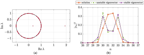
Figure 4. (a) Floquet eigenvalues of an exact stationary polarobreather. The unstable eigenvalues are so large and small because the common period $T_F$ is 16 times the breather period and 9 times the probability period. (b) Profile of the charge probability and the stable and unstable eigenvectors of the charge probability, where the latter corresponds to the switching mode. See text.

Long-time simulations confirm this interpretation. After some time, the polarobreather switches a position; after some time, it switches back, and so on. Therefore, in spite of the instability, which gets stabilized by the nonlinearity of the lattice, the breather and charge probability are stationary. They do not disperse or travel, but experience quasi-periodic switches between two neighboring sites. Figure 5 shows the switching behavior of a polarobreather in a long-time simulation.

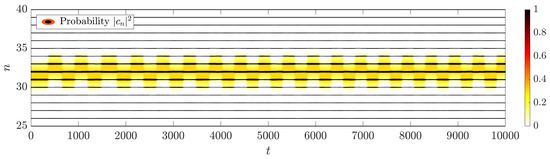
Figure 5. Long-time simulation of an exact stationary polarobreather. The alternating switching of position and charge can be observed.

10. Moving Polarobreathers

In this section, we follow the scheme of the previous section on stationary polarobreathers. In spite of the additional complications by the mobility, this will be easy to explain based on that section.

10.1. Generation of Approximate Moving Polarobreathers

The method used to produce moving polarobreathers in this model is also extremely efficient. We introduce as initial conditions the following initial pattern for the momenta or velocities:

$${(p_{n^{*}-1},p_{n^{*}},p_{n^{*}+1})}^T=\gamma {(-1,2,-1)}^T,\gamma \in {\mathbb{R}}_{\ne 0},$$

while the particle displacements are set at zero. The parameter $\gamma$ is a measure of the modulus of the initial kinetic energy $K_E=3{\gamma }^2$. The charge amplitude function with a probability of one is initially located with the pattern (51).

Figure 6-top shows the $XTFT$ plots obtained with $\gamma =0.6$, $K_E=1.08$. They look very similar to Figure 2-top. As already seen in Section 4, the transformation ${\omega }_L\to {\omega }_M={\omega }_L-q{V}_b$ corresponds to the description of the system in the comoving frame, where all the phonons and excitations traveling at the same velocity $V_b$ appear as horizontal lines, corresponding to a stationary solution with a single frequency. Quite a few bands appear. For $u_n$ and $|c_n{|}^2$, real numbers, we only comment on the positive part of the spectrum due to its symmetry. One necessary objective to obtain moving exact polarobreathers is to identify the common fundamental time $T_F$ and step s.

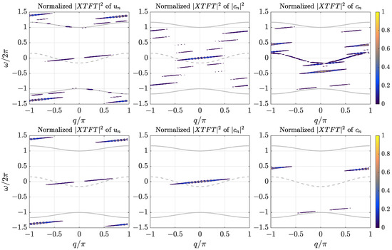
Figure 6. (Top) $XTFT$ of $u_n$, $|c_n{|}^2$ and $c_n$ for an approximate polarobreather generated with $\gamma =0.6$ and kinetic energy $K_E=1.08$. (Bottom) $XTFT$ of $u_n$, $|c_n{|}^2$ and $c_n$ for the exact moving polarobreather obtained using the approximate polarobreather as an initial seed. See text.

• We observe the $XTFT$ of $u_n$. There are three localized waves traveling at the same speed, and some phonons. The three localized waves are a soliton; a breather; and with weaker intensity, what we could call a quasilinear breather, very close to the phonon band. We know that the soliton and main breather are characteristic components of this system, with strong asymmetry in the coupling potential. Therefore, we discard the weaker breather as an effect of the breather not being exact. In Section 4 it is deduced that the breather frequency in the moving frame ${\Omega }_L$ is the frequency of the breather line for $q=0$. The commensurability relation (17) was also obtained:

  $$\frac{{\Omega }_L}{2\pi V_b}=\frac{m_L{\omega }_F}{s_L{\omega }_F}=\frac{m_L}{s_L},$$

  with $m_L$ and the step $s_L$ being the integers we have to find. We measure ${\Omega }_L/2\pi \simeq 1.2257$ and $V_b\simeq 0.3065$; then ${\Omega }_L/2\pi V_b=3.999\simeq 4$. Therefore, the simplest values are

  $$m_L=4,s_L=1,\frac{{\omega }_{F,L}}{2\pi }\simeq 0.3065,T_{F,L}\simeq 3.2626.$$
• For the $XTFT$ of $|c_n{|}^2$, also for positive frequencies, we observe four resonant lines with intensity. One is the soliton, characteristic of the $XTFT$ of a positive quantity. The many lines are a sign of high nonlinearity, which corresponds to a very localized $|c_n{|}^2$, and is therefore close to one for some n. The linear approximation is not at all valid, and there are many harmonic frequencies.
• For the $XTFT$ of $c_n$, we have to observe the frequency differences, as the solution is invariant to a global shift in frequency, as explained in Section 3. We observe many phonons in the dispersion band, two positive bands centered around $q=\pm \pi$, and two negative bands centered at $q=0$. Two bands are very close to the phonon band, indicating a strong interaction with the linear modes. Observing the two truly nonlinear bands, their difference in frequency is ${\Omega }_c/2\pi \simeq 0.715$, corresponding to ${\Omega }_c=m_c{\omega }_{F,c}$. Using the commensurability relation (17) as above and with the same $V_b\simeq 0.3064$, we obtain:

  $$\frac{{\Omega }_c}{2\pi V_b}=\frac{m_c}{s_c}\simeq \frac{7}{3}.$$
  We conclude that

  $$m_c=7,s_c=3,\frac{{\omega }_{F,c}}{2\pi }\simeq 0.1021,T_{F,c}\simeq 9.7911.$$
  Thus, we can set the common step $s=3$ and estimate the fundamental time $T_F=9.79$, i.e.,

  $$T_F=9.79\simeq 3T_{F,L}\simeq T_{F,c},$$

  as well as finding an approximate value of $E_0\simeq 0.0028$ for the computation of the exact moving polarobreathers of the following section.

10.2. Exact Moving Polarobreathers

Using the numerical methods explained in Section 8 and the found step s and fundamental period $T_F$, together with the estimated $E_0$ value, we can obtain numerically exact moving polarobreathers. Their $XTFT$ is shown in Figure 6-bottom. There is a large difference between the approximate moving polarobreather and the exact one.

• For the $XTFT$ of $u_n$, phonons have been eliminated, and only a well localized soliton breather remains.
• For the $XTFT$ of $|c_n{|}^2$, only a soliton remains, meaning that in the moving frame, it is reduced to a static deformation, corresponding to a charge probability traveling without vibration. The other part of the solution is a uniform probability spread through the lattice, indicating a small probability that the charge could appear at any site n.
• For the $XTFT$ of $c_n$, two intensity bands remain: one around $q=0$, and a stronger one centered at $q=\pm \pi$. The difference in frequencies is exactly the breather frequency, indicating that there is no vibration of $c_n$, except the one driven by the change in the transfer elements $J_{n,n+1}$, which depend on $u_n$.

To summarize, there is a common fundamental period $T_F$, during which the polarobreather repeats itself with a shift of $s=3$ sites. In $T_F$, the breather at $u_n$ repeats three times, and in the moving frame performs $m_L=4$ oscillations for each repetition, totaling 12 repetitions. In the same duration of time $T_F$, the $c_n$ variable oscillates $m_c=7$ times, while advancing $s_c=3$ sites. There is no vibration in $|c_n{|}^2$; there is just the translation with velocity $V_b$ of the static profile with about half the probability located at a single site, and the rest is uniformly shared by the rest of lattice particles. The periodicity of the exact polarobreather solution can be appreciated in Figure 7, where the particle displacements $u_n$ (Figure 7a) and the charge probability $|c_n{|}^2$ (Figure 7b) are illustrated in time separated by five fundamental periods $T_F=9.79$.

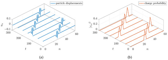
Figure 7. Profiles of an exact moving polarobreather in time separated by 5 fundamental periods $T_F=9.79$. (a) $u_n$, with high localization and staggered profile. (b) $|c_n{|}^2$, corresponding to a charge probability localized at five sites and peaking at one site.

10.3. Stability of Moving Polarobreathers

Most of the properties for the eigenvalues of the Floquet matrix for the moving exact polarobreather are the same as in the stationary case (see Section 9.3), as we are observing the system in the moving frame where it is stationary. Eigenvalues of the Floquet matrix are illustrated in Figure 8. There is also a difference; now, we should expect six structural eigenvalues at the eigenvalue $(1,0)$. They correspond to the growth and phase mode for $u_n$ and $c_n$, and two new eigenvalues associated with a small change of the velocity. The latter imply that there exists another solution with a small change in the velocity $V_b$. This solution will not be an exact solution that will appear with the change in $T_F$ for constant s. The stability of the exact moving polarobreather can be observed in a very long-time simulation, shown in Figure 9.

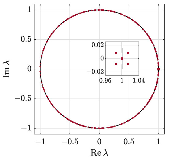
Figure 8. Floquet eigenvalues for the moving exact polarobreather. The six structural eigenvalues at $(1,0)$ can be seen, with some imprecision due to the numerical error and the long time used for the common $T_F$ for all the variables. See text.

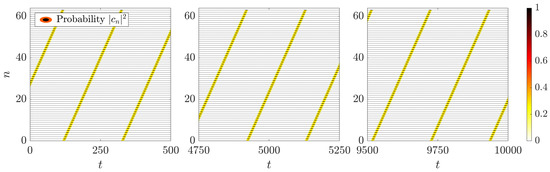
Figure 9. Long-time simulation of an exact moving polarobreather showing its stability.

10.4. Path Continuation

By changing the parameters $T_F$ and keeping the step and the ratio between the $u_n$ and $c_n$ periods, it is possible to obtain exact solutions with similar characteristics with a different fundamental frequency ${\omega }_F$, both for increasing and decreasing frequencies. For the decreasing frequencies, the convergence stops as the $u_n$ frequency approaches the phonon band. For increasing frequencies, the path continuation also eventually stops to converge. These results will be published elsewhere.

11. Conclusions

We considered a classical model without charge that shows long-lived traveling breathers, and used it to construct a semiclassical model adding the coupling to a charged quantum particle—electron or hole. We analyzed the system and advanced its properties through linear and tail analysis. We adapted recent numerical methods developed by the authors to produce efficient symplectic algorithms that preserve symplecticity and charge conservation at every time step. They allow for efficient integration of the dynamical equations without the Born–Oppenheimer approximation, i.e., both the lattice and the charge are out of equilibrium. We constructed initial conditions for the lattice variables and the charge amplitude that bring about long-lived polarobreathers. The analysis of their spectra allows important parameters to be obtained not only for exact stationary solutions, but in particular for traveling ones, such as the step, fundamental frequency, and frequency in the moving frame, both for the lattice and charge variables. We developed a method for obtaining numerically exact polarobreathers, using as an initial seed the approximate solutions and the parameters found in their spectra. An important aspect of this method is dealing with the system invariance under a change in the frequency of the charge amplitude. The spectrum of the exact polarobreathers is much more simplified, leaving only a breather and a soliton for the lattice variables, a soliton for the charge probability, and two breather-like exact solutions for the charge amplitude, with a frequency difference that matches the breather one and corresponds to a soliton and a breather with a frequency shift. However, for approximate polarobreathers that might appear in real systems, the charge probability shows small oscillations with frequencies that can be related to the frequencies of the charge amplitude. The obtained results may allow for the identification of charge coupling and its properties in the spectrum of real systems.

References

- Landau, L.D. Electron motion in crystal lattices. Phys. Z. Sowjetunion 1933, 3, 664. [Google Scholar]
- Landau, L.D.; Pekar, S.I. Effective mass of a polaron. Zh. Eksp. Teor. Fiz. 1948, 18, 419–423, English translation: Ukr. J. Phys. 2008, 53, 71–74. [Google Scholar]
- Holstein, T. Studies of polaron motion: Part I. The molecular-crystal model. Ann. Phys. 1959, 8, 325–342. [Google Scholar] [CrossRef]
- Holstein, T. Studies of polaron motion: Part II. The “small” polaron. Ann. Phys. 1959, 8, 343–389. [Google Scholar] [CrossRef]
- Alexandrov, A.S. Polarons in Advanced Materials; Springer: Dordrecht, The Netherlands, 2007. [Google Scholar]
- Dubinko, V.I.; Selyshchev, P.A.; Archilla, J.F.R. Reaction-rate theory with account of the crystal anharmonicity. Phys. Rev. E 2011, 83, 041124. [Google Scholar] [CrossRef]
- Davydov, A.S. Solitons in Molecular Systems; Mathematics and Its Applications; Springer: Dordrecht, The Netherlands, 1985. [Google Scholar]
- Remoissenet, M. Waves Called Solitons; Advanced Texts in Physics; Springer: Berlin, Germany, 1999. [Google Scholar]
- Sievers, A.J.; Takeno, S. Intrinsic Localized Modes in Anharmonic Crystals. Phys. Rev. Lett. 1988, 61, 970–973. [Google Scholar] [CrossRef]
- Sato, M.; Sievers, A.J. Direct observation of the discrete character of intrinsic localized modes in an antiferromagnet. Nature 2004, 432, 486–488. [Google Scholar] [CrossRef]
- Flach, S.; Gorbach, A.V. Discrete breathers. Advances in theory and applications. Phys. Rep. 2008, 467, 1–116. [Google Scholar] [CrossRef]
- MacKay, R.S.; Aubry, S. Proof of Existence of Breathers for Time-Reversible or Hamiltonian Networks of Weakly Coupled Oscillators. Nonlinearity 1994, 7, 1623. [Google Scholar] [CrossRef]
- Marín, J.L.; Aubry, S. Breathers in Nonlinear Lattices: Numerical Calculation from the Anticontinuous Limit. Nonlinearity 1996, 9, 1501. [Google Scholar] [CrossRef]
- Aubry, S. Breathers in nonlinear lattices: Existence, linear stability and quantization. Physica D 1997, 103, 1–4. [Google Scholar] [CrossRef]
- MacKay, R.S.; Sepulchre, J.A. Stability of discrete breathers. Physica D 1998, 119, 148–162. [Google Scholar] [CrossRef]
- Yoshimura, K.; Doi, Y. Moving discrete breathers in nonlinear lattice: Resonance and stability. Wave Motion 2007, 45, 83–99. [Google Scholar] [CrossRef]
- Butt, I.A.; Wattis, J.A.D. Asymptotic analysis of combined breather-kink modes in a Fermi-Pasta-Ulam chain. Physica D 2007, 231, 165–179. [Google Scholar] [CrossRef]
- Chong, C.; Kevrekidis, P.G.; Theocharis, G.; Daraio, C. Dark breathers in granular crystals. Phys. Rev. E 2013, 87, 042202. [Google Scholar] [CrossRef]
- Koukouloyannis, V. Seminumerical method for tracking multibreathers in Klein-Gordon chains. Phys. Rev. E 2004, 69, 046613. [Google Scholar] [CrossRef]
- Lazarides, N.; Eleftheriou, M.; Tsironis, G.P. Discrete breathers in nonlinear magnetic metamaterials. Phys. Rev. Lett. 2006, 97, 157406. [Google Scholar] [CrossRef]
- Haas, M.; Hizhnyakov, V.; Shelkan, A.; Klopov, M.; Sievers, A.J. Prediction of high-frequency intrinsic localized modes in Ni and Nb. Phys. Rev. B 2011, 84, 144303. [Google Scholar] [CrossRef]
- Hizhnyakov, V.; Haas, M.; Shelkan, A.; Klopov, M. Theory and molecular dynamics simulations of intrinsic localized modes and defect formation in solids. Phys. Scr. 2014, 89, 044003. [Google Scholar] [CrossRef]
- Chechin, G.M.; Dmitriev, S.V.; Lobzenko, I.P.; Ryabov, D.S. Properties of discrete breathers in graphane from ab initio simulations. Phys. Rev. B 2014, 90, 045432. [Google Scholar] [CrossRef]
- Lobzenko, I.P.; Chechin, G.M.; Bezuglova, G.S.; Baimova, Y.A.; Korznikova, E.A.; Dmitriev, S.V. Ab initio simulation of gap discrete breathers in strained graphene. Phys. Solid State 2016, 58, 633–639. [Google Scholar] [CrossRef]
- Archilla, J.F.R.; Doi, Y.; Kimura, M. Pterobreathers in a model for a layered crystal with realistic potentials: Exact moving breathers in a moving frame. Phys. Rev. E 2019, 100, 022206. [Google Scholar] [CrossRef] [PubMed]
- Bajārs, J.; Archilla, J.F.R. Frequency-momentum representation of moving breathers in a two dimensional hexagonal lattice. Physica D 2022, 441, 133497. [Google Scholar] [CrossRef]
- Kalosakas, G.; Aubry, S. Polarobreathers in a generalized Holstein model. Physica D 1998, 113, 228–232. [Google Scholar] [CrossRef]
- Cuevas, J.; Kevrekidis, P.G.; Frantzeskakis, D.J.; Bishop, A.R. Existence of bound states of a polaron with a breather in soft potentials. Phys. Rev. B 2006, 74, 064304. [Google Scholar] [CrossRef]
- Chetverikov, A.P.; Ebeling, W.; Velarde, M.G. Nonlinear soliton-like excitations in two-dimensional lattices and charge transport. Eur. Phys. J.-Spec. Top. 2013, 222, 2531–2546. [Google Scholar] [CrossRef]
- Velarde, M.G.; Ebeling, W.; Chetverikov, A.P. Thermal solitons and solectrons in 1D anharmonic lattices up to physiological temperatures. Int. J. Bifurc. Chaos 2008, 18, 3815–3823. [Google Scholar] [CrossRef]
- Ros, O.G.C.; Cruzeiro, L.; Velarde, M.G.; Ebeling, W. On the possibility of electric transport mediated by long living intrinsic localized solectron modes. Eur. Phys. J. B 2011, 80, 545–554. [Google Scholar]
- Ashcroft, N.W.; Mermim, N.D. Solid State Physics, 1st ed.; Cengage Learning: Boston, MA, USA, 1976. [Google Scholar]
- Bajārs, J.; Archilla, J.F.R. Splitting methods for semi-classical Hamiltonian dynamics of charge transfer in nonlinear lattices. Mathematics 2022, 10, 3460. [Google Scholar] [CrossRef]
- Russell, F.M.; Archilla, J.F.R.; Frutos, F.; Medina-Carrasco, S. Infinite charge mobility in muscovite at 300 K. EPL 2017, 120, 46001. [Google Scholar] [CrossRef]
- Russell, F.M.; Russell, A.W.; Archilla, J.F.R. Hyperconductivity in fluorphlogopite at 300 K and 1.1 T. EPL 2019, 127, 16001. [Google Scholar] [CrossRef]
- Braun, O.M.; Kivshar, Y.S. Nonlinear dynamics of the Frenkel-Kontorova model. Phys. Rep. 1998, 1–2, 1–108. [Google Scholar] [CrossRef]
- Braun, O.M.; Kivshar, Y.S. The Frenkel-Kontorova Model; Springer: Berlin/Heidelberg, Germany, 2004. [Google Scholar]
- Bajars, J.; Eilbeck, J.C.; Leimkuhler, B. Nonlinear propagating localized modes in a 2D hexagonal crystal lattice. Physica D 2015, 301–302, 8–20. [Google Scholar] [CrossRef]
- Bajars, J.; Eilbeck, J.C.; Leimkuhler, B. 2D mobile breather scattering in a hexagonal crystal lattice. Phys. Rev. E 2021, 103, 022212. [Google Scholar] [CrossRef]
- Cohen-Tannoudji, C.; Diu, B.; Laloe, F. Quantum Mechanics, Volume 1: Basic Concepts, Tools, and Applications, 2nd ed.; Wiley-VCH: Weinheim, Germany, 2019. [Google Scholar]
- Archilla, J.F.; Zolotaryuk, Y.; Kosevich, Y.A.; Doi, Y. Nonlinear waves in a model for silicate layers. Chaos 2018, 28, 083119. [Google Scholar] [CrossRef]
- Boyd, J.P. A numerical calculation of a weakly nonlocal solitary wave: The ϕ4 breather. Nonlinearity 1990, 3, 177–195. [Google Scholar] [CrossRef]
- Hairer, E.; Lubich, C.; Wanner, G. Geometrical Numerical Integration: Structure-Preserving Algorithms for Ordinary Differential Equations, 2nd ed.; Springer Series in Computational Mathematics; Springer: Berlin/Heidelberg, Germany, 2006; Volume 31. [Google Scholar]
- Blanes, S.; Casas, F.; Murua, A. Splitting and composition methods in the numerical integration of differential equations. Bol. Soc. Esp. Mat. Apl. 2008, 45, 89–145. [Google Scholar]
- Nocedal, J.; Wright, S.J. Numerical Optimization; Springer Series in Operations Research and Financial Engineering; Springer: New York, NY, USA, 2006. [Google Scholar]
Disclaimer/Publisher’s Note: The statements, opinions and data contained in all publications are solely those of the individual author(s) and contributor(s) and not of MDPI and/or the editor(s). MDPI and/or the editor(s) disclaim responsibility for any injury to people or property resulting from any ideas, methods, instructions or products referred to in the content. |
© 2023 by the authors. Licensee MDPI, Basel, Switzerland. This article is an open access article distributed under the terms and conditions of the Creative Commons Attribution (CC BY) license (https://creativecommons.org/licenses/by/4.0/).