Partially Linear Additive Hazards Regression for Bivariate Interval-Censored Data

Abstract

In this paper, we discuss regression analysis of bivariate interval-censored failure time data that often occur in biomedical and epidemiological studies. To solve this problem, we propose a kind of general and flexible copula-based semiparametric partly linear additive hazards models that can allow for both time-dependent covariates and possible nonlinear effects. For inference, a sieve maximum likelihood estimation approach based on Bernstein polynomials is proposed to estimate the baseline hazard functions and nonlinear covariate effects. The resulting estimators of regression parameters are shown to be consistent, asymptotically efficient and normal. A simulation study is conducted to assess the finite-sample performance of this method and the results show that it is effective in practice. Moreover, an illustration is provided.

1. Introduction

In this article, we discuss a regression analysis using the marginal additive hazards model on bivariate interval-censored data. Interval-censored data refer to failure times that are observed to only belong to an interval rather than being known with absolute certainty. These types of data frequently occur in various areas, including biomedical and epidemiological investigations [1]. It is easy to see that the most commonly studied right-censored data can be seen as a special case of interval-censored data, and it is important to note that the analysis of interval-censored data is typically far more difficult than right-censored data research. Bivariate interval-censored data occur when there exist two correlated failure times of interest and the observed times of both failure events suffer interval censoring. Clinical trials or medical studies on several events from the same individual such as eye disease studies often yield bivariate interval-censored data. The purpose of this article is to propose a flexible regression model which can process bivariate interval-censored data when the main interest is on the risk differential or excess risk.

There are several methods available for regression analysis of univariate interval-censored data arising from the additive hazards model. Refs. [2,3], for example, investigated the problem for case I interval-censored or current state data, a special form of interval-censored data in which the observed time contains zero or infinite. The former discussed an estimating equation approach and the latter considered an efficient estimation approach. More recently, Ref. [4] studied the same issue as Ref. [2] but with some inequality constraints, and Ref. [5] proposed a sieve maximum likelihood approach. Moreover, Ref. [6] developed several inverse probability weight-based and reweighting-based estimation procedures for the situation with missing covariates, while Ref. [7] presented an efficient approach for general situations.

A large number of approaches have been established for modeling bivariate interval-censored survival data and three types of methods are generally used. One is a marginal method that relies on the working independence assumption [8,9]. Another commonly used approach is the frailty-model-based method, which employs the frailty or latent variable to build the correlation among the associated failure times [10,11]. Ref. [12] proposed a frailty model method for multivariate interval-censored data with informative censoring. The third type of method is the copula-based approach, which gives a different, specific way to model two dependent failure times. One advantage of the approach is that it directly connects the two marginal distributions through a copula function to construct the joint distribution and uses the copula parameter to determine the correlation. This distinguishing characteristic makes it possible to represent the margins independent of the copula function. This advantage is appealing for the points of both modeling and interpretation views. Among others, Ref. [13] discussed this approach based on the marginal transformation model with the two-parameter Archimedean copula. Ref. [14] proposed a copula link-based additive model for right-censored event time data. Moreover, Ref. [15] proposed a copula-based model to deal with bivariate survival data with various censoring mechanisms. In the following, we discuss the regression analysis of bivariate cases by employing the method in [13]. More specifically, we propose a kind of semiparametric partly linear additive hazards model.

Partly linear models are becoming more and more common since they combine the flexibility of nonparametric modeling with the simplicity and ease of interpretation of parametric modeling. It is presumptive that the marginally conditional hazard function has nonlinear relationships with some covariates but linear relationships with others [16,17,18]. In practice, nonlinear covariate effects are typical. For instance, in some medication research, the influence of the dosage of a particular medication may reach a peak at a certain dosage level and be maintained at the peak level, or it may diminish after the dosage level. Although there is a fair amount of literature in this field, to the best of our knowledge, there does not seem to exist a study considering this for bivariate interval-censored survival data.

The presented model involves two nonparametric functions, one identifies the baseline cumulative hazard function and another describes the nonlinear effects of a continuous covariate. In the following, the two-parameter Archimedean copula model is employed for the dependence and more comments on this is given below. Moreover, a sieve maximum likelihood estimation approach is developed to approximate two involved nonparametric nuisance functions by Bernstein polynomials. The proposed method has several desirable features: (a) it allows both time-dependent covariates and the covariates that may have nonlinear effects; (b) the two-parameter Archimedean copula model can flexibly handle dependence structures on both upper and lower tails and the strength of the dependence can be quantified via Kendall’s $\tau$; (c) the sieve maximum likelihood estimation approach by Bernstein polynomials can be easily implemented with the use of some existing software; (d) as is seen in the simulation study, the computation is both stable and efficient. Note that the method given by [13] only allows for linear covariate effects.

More specifically, in Section 2, after recommending some notation, assumptions and models that would be used throughout the paper, the resulting likelihood function is presented. In Section 3, we first describe the proposed sieve maximum likelihood estimation approach and then present the asymptotic properties of the proposed estimators. Section 4 presents a simulation study for the assessment of the finite sample performance of the proposed estimation approach, and the results indicate that it works well as expected. In Section 5, an illustration is provided by using a set of data arising from the Age-Related Eye Disease Study (AREDS), and Section 6 gives the conclusion with some discussion and concluding remarks.

2. Assumptions and Likelihood Function

Consider a study consisting of n independent subjects. Define $T_{ij}$ as the failure time of interest associated with the ith subject of the jth failure event. Suppose that for $T_{ij}$, the two observation times are given by $(U_{ij},V_{ij}]$ such that $U_{ij}<T_{ij}\le V_{ij}$. In addition, suppose that for the ith subject, the p-dimensional covariate vectors are possibly time-dependent and denoted by $X_{i1}$ and $X_{i2}$ and the single continuous covariates $Z_{i1}$ and $Z_{i2}$ are related to $T_{i1}$ and $T_{i2}$, respectively. More details on them are given below. Here, we assume that $X_{i1}$ and $X_{i2}$ or $Z_{i1}$ and $Z_{i2}$ could be the same, entirely different, or they also could have some common components. Then, the observed data are as follows:

$$O=\{O_i=\left(U_{ij},V_{ij},X_{ij},Z_{ij}\right);i=1,\dots ,n,j=1,2\}.$$

Note that when $V_{ij}=\infty , T_{ij}$ is right-censored and when $U_{ij}=0, T_{ij}$ is left-censored. Moreover, it is assumed that given the covariates, the interval censoring is independent of the failure times $T_{ij}$ [1].

Given some covariates, define $S_{ij}\left(t_{ij}|X_{ij},Z_{ij}\right)=P\left(T_{ij}>t_{ij}|X_{ij},Z_{ij}\right)$ as the marginal survival function of $T_{ij}$, and

$$S\left(t_{i1},t_{i2}|X_{i1},X_{i2},Z_{i1},Z_{i2}\right)=P\left(T_{i1}>t_{i1},T_{i2}>t_{i2}|X_{i1},X_{i2},Z_{i1},Z_{i2}\right),$$

is the joint survival function of $T_{i1}$ and $T_{i2}$. For the covariate effects, suppose that given $X_{ij}$ and $Z_{ij}$, the marginal hazard function of $T_{ij}$ is defined as follows:

$$h_j(t|X_{ij},Z_{ij})={\lambda }_j(t)+{\beta }^T{X}_{ij}(t)+g(Z_{ij}),$$

where ${\lambda }_j(t)$ denotes an unknown baseline hazard function, $\beta$ is an unknown regression coefficient vector, and $g(·)$ is an unknown, smooth nonlinear regression function. That is, $T_{ij}$ follows a partially linear additive hazards model, in which $Z_{ij}$ represents the covariate that may have nonlinear effects on $T_{ij}$. Correspondingly, $T_{ij}$ has the cumulative hazard

$$H_j(t|X_{ij},Z_{ij})={\int }_0^t{h}_j(s|X_{ij},Z_{ij})ds={\mathsf{\Lambda }}_j(t)+{\beta }^T{W}_{ij}(t)+g(Z_{ij})t,$$

where ${\mathsf{\Lambda }}_j(t)={\int }_0^t{\lambda }_j(s)ds$, $W_{ij}(t)={\int }_0^t{X}_{ij}(s)ds$, and we have that

$$\begin{array}{cc}\hfill & S_{ij}(t|X_{ij},Z_{ij})=exp[-{\int }_0^t{h}_j(s|X_{ij},Z_{ij})ds]=exp[-H_j(t;X_{ij},Z_{ij})]\hfill \\ \hfill & =exp\left[-\{{\mathsf{\Lambda }}_j(t)+{\beta }^T{W}_{ij}(t)+g(Z_{ij})t\}\right],i=1,\cdots ,n,j=1,2,\hfill \end{array}$$

(1)

It is worth noting that for the simplicity of the expressions and calculations, we assume that both linear and nonlinear covariates effects are the same for the two associated failure times of interest [19,20]. It is simple to extend the following method to the situation where the covariate effects are different.

It follows from Sklar’s theorem [21] that if the marginal survival functions $S_{ij}(·)$ are continuous, there exists a unique copula function $C_{\xi }(·,·)$ on ${[0,1]}^2$ such that $C_{\xi }(s_1,0)=C_{\xi }(0,s_2)=0$, $C_{\xi }(s_1,1)=s_1$ and $C_{\xi }(1,s_2)=s_2$, and it gives

$$S\left(t_{i1},t_{i2}|X_{i1},X_{i2},Z_{i1},Z_{i2}\right)=C_{\xi }\left(S_{i1}\left(t_{i1}|X_{i1},Z_{i1}\right),S_{i2}\left(t_{i2}|X_{i2},Z_{i2}\right)\right),t_{i1},t_{i2}⩾0.$$

Here, the parameter $\xi$ generally denotes the correlation or dependence between $T_{i1}$ and $T_{i2}$. As mentioned above, a significant advantage of the copula representation above is that it separates the correlation from the two marginal distributions [22]. There exist many copula functions and among others, one type of the most commonly used copula functions for bivariate data is perhaps the Archimedean copula family. By following [13], we focus on the flexible two-parameter Archimedean copula model given by

$$\begin{array}{cc}\hfill C_{\phi ,\omega }(s_1,s_2)& ={\left[1+{\left\{{\left(s_1^{-1/\omega }-1\right)}^{1/\phi }+{\left(s_2^{-1/\omega }-1\right)}^{1/\phi }\right\}}^{\phi }\right]}^{-\omega }\hfill \\ \hfill & =\mu \left({\mu }^{-1}(s_1)+{\mu }^{-1}(s_2)\right),\phi \in (0,1],\omega \in (0,\infty ),\hfill \end{array}$$

(2)

where $\mu (s)={\mu }_{\phi ,\omega }(s)={\left(1+s^{\phi }\right)}^{-\omega }$ and ${\mu }^{-}$ is the generalized inverse of $\mu$, which is defined as ${\mu }^{-}(y)=inf\{x\in \mathbb{R}:y\le \mu (x)\},y\in \mathbb{R}$. The detailed derivation and more comments can be found in Chapter 5 of [23].

As mentioned before, the two parameters $\phi$ and $\omega$ in the copula function above are the association parameters, representing the correlation in both the upper and lower tails. In particular, when $\phi =1,$ the copula model above is equal to the Clayton copula [24], while if $\omega \to \infty$, the copula model becomes the Gumbel copula [25]. In other words, the two-parameter copula model is more flexible and has the Clayton or Gumbel copula as special cases. It is well-known that another commonly used measure for the correlation is Kendall’s $\tau$, and it has an explicit connection with $\phi$, $\omega$ as

$$\tau =1-2\phi \omega /(2\omega +1).$$

Under the assumptions above, the observed likelihood function has the form

$$\begin{array}{cc}\hfill & L_n\left(S_1,S_2,\phi ,\omega |O\right)=\prod _{i=1}^{n}P\left(U_{i1}<T_{i1}⩽V_{i1},U_{i2}<T_{i2}⩽V_{i2}|Y_{i1},Y_{i2}\right)\hfill \\ \hfill & =\prod _{i=1}^n\left\{P\left(T_{i1}>U_{i1},T_{i2}>U_{i2}|Y_{i1},Y_{i2}\right)-P\left(T_{i1}>U_{i1},T_{i2}>V_{i2}|Y_{i1},Y_{i2}\right)\right.\hfill \\ \hfill & \left.-P\left(T_{i1}>V_{i1},T_{i2}>U_{i2}|Y_{i1},Y_{i2}\right)+P\left(T_{i1}>V_{i1},T_{i2}>V_{i2}|Y_{i1},Y_{i2}\right)\right\}\hfill \\ \hfill & =\prod _{i=1}^n\left\{S\left(U_{i1},U_{i2}|Y_{i1},Y_{i2}\right)-S\left(U_{i1},V_{i2}|Y_{i1},Y_{i2}\right)-S\left(V_{i1},U_{i2}|Y_{i1},Y_{i2}\right)\right.\hfill \\ \hfill & \left.+S\left(V_{i1},V_{i2}|Y_{i1},Y_{i2}\right)\right\}\hfill \\ \hfill & =\prod _{i=1}^n\left\{C_{\phi ,\omega }\left[S_1\left(U_{i1}|Y_{i1}\right),S_2\left(U_{i2}|Y_{i2}\right)\right]-C_{\phi ,\omega }\left[S_1\left(U_{i1}|Y_{i1}\right),S_2\left(V_{i2}|Y_{i2}\right)\right]\right.\hfill \\ \hfill & \left.-C_{\phi ,\omega }\left[S_1\left(V_{i1}|Y_{i1}\right),S_2\left(U_{i2}|Y_{i2}\right)\right]+C_{\phi ,\omega }\left[S_1\left(V_{i1}|Y_{i1}\right),S_2\left(V_{i2}|Y_{i2}\right)\right]\right\},\hfill \end{array}$$

(3)

where $Y_{i1}=(X_{i1},Z_{i1}),Y_{i2}=(X_{i2},Z_{i2})$. Let $\eta =\left(\beta ,\phi ,\omega ,{\mathsf{\Lambda }}_1,{\mathsf{\Lambda }}_2,g\right)$, all unknown parameters. The next section proposes a sieve approach for the estimation of $\eta$.

3. Sieve Maximum Likelihood Estimation

It is well-known that directly maximizing the likelihood function $L_n(\eta |O)=L_n(S_1,S_2,\phi ,$$\omega |O)={\sum }_{i=1}^{n}L(\eta ;O_i)$ can provide an estimate of $\eta$. On the other hand, it is inappropriate for this situation, as it involves infinite-dimensional functions ${\mathsf{\Lambda }}_j(t)$ and $g(·)$. For this, according to [26] and others, we suggest using the sieve method to approximate these functions based on Bernstein’s polynomial first, and then maximize the likelihood function.

Specifically, define $\mathsf{\Theta }=\mathcal{A}\otimes \mathcal{M}\otimes \mathcal{M}\otimes \mathcal{G}$, the parameter space, and

$$\mathcal{A}=\left\{\left(\beta ,\phi ,\omega \right)\in R^p\times R^{(0,1]}\times R^{+},\parallel \beta \parallel +\parallel \phi \parallel +\parallel \omega \parallel \le K\right\},$$

in which ⊗ denotes the Kronecker product, and K is a nonnegative constant. Additionally, $\mathcal{M}$ denotes the subset of all bounded and continuous, nondecreasing, nonnegative functions within $[c_1,d_1]$, $0⩽c_1<d_1<\infty$. Similarly, $\mathcal{G}$ denotes the collection of all bounded and continuous functions within $[c_2,d_2]$, the support of $Z_{ij}$. In practice, $[c_1,d_1]$ is generally valued as the large and minimum values of all observation times. In the following, define the sieve parameter space

$${\mathsf{\Theta }}_n=\left\{{\eta }_n={\left({\beta }^T,\phi ,\omega ,{\mathsf{\Lambda }}_{n1},{\mathsf{\Lambda }}_{n2},g_n\right)}^T\in \mathcal{A}\otimes {\mathcal{M}}_n\otimes {\mathcal{M}}_n\otimes {\mathcal{G}}_n\right\}.$$

In the above,

$${\mathcal{M}}_n=\{{\mathsf{\Lambda }}_{nj}(t)=\sum _{k=0}^{m_1}{\varphi }_{jl}^{*}{B}_l\left(t,m_1,c_1,d_1\right):\sum _{l=0}^{m_1}{\varphi }_{jl}^{*}⩽M_n;0⩽{\varphi }_{j0}^{*}⩽\cdots ⩽{\varphi }_{j{m}_1}^{*};j=1,2\},$$

and

$${\mathcal{G}}_n=\{g_n(z)=\sum _{k=0}^{m_2}{\alpha }_k{B}_k\left(z,m_2,c_2,d_2\right):\sum _{k=0}^{m_2}\left|{\alpha }_k\right|⩽G_n\}$$

with

$$B_k\left(x,m,c,d\right)=\left(\begin{array}{c}m\\ k\end{array}\right){\left(\frac{x-c}{d-c}\right)}^k{\left(1-\frac{x-c}{d-c}\right)}^{m-k},k=0,\cdots ,m,$$

the Bernstein basis polynomial with the degrees $m_1=O\left(n^{{\nu }_1}\right)$ and $m_2=O\left(n^{{\nu }_2}\right)$ for some fixed ${\nu }_1,{\nu }_2\in (0,1)$, and $M_n$ and $G_n$ being some positive constants. To estimate $\eta$, define ${\widehat{\eta }}_n=({\widehat{\beta }}_n,{\widehat{\phi }}_n,{\widehat{\omega }}_n,{\widehat{\mathsf{\Lambda }}}_{n1},{\widehat{\mathsf{\Lambda }}}_{n2},\widehat{g})$ as the value of $\eta$ by maximizing the log-likelihood function

$${\ell }_n(\eta ;O)=log{L}_n(\eta ;O)=\sum _{i=1}^{n}logL\left(\eta ;O_i\right).$$

(4)

Note that one of the main advantages of Bernstein polynomials is that they can easily implement the nonnegativity and monotonicity properties of ${\mathsf{\Lambda }}_j(t)$ by the reparameterization ${\varphi }_{j0}^{*}=e^{{\varphi }_{j0}}$, ${\varphi }_{jl}^{*}={\sum }_{i=0}^l{e}^{{\varphi }_{ji}},\forall 1\le l\le m_1$ [26]. In addition, of all approximation polynomials, they have the optimal shape-preserving properties [27]. By the way, they are easy to use because they do not need interior knots. In the above, for simplicity, the same basis polynomial is used for ${\mathsf{\Lambda }}_1$ and ${\mathsf{\Lambda }}_2$. Moreover, note that this approach can be relatively easily implemented as discussed below, although it may seem to be complicated. In practice, one need to choose $m_j(j=1,2)$. We suggest employing the Akaike information criterion (AIC) defined as

$$\mathrm{AIC}=-2{\ell }_n({\widehat{\eta }}_n)+2\left(p+m_1+m_2+2+2\right).$$

In the above, the form in the second bracket is the number of unknown parameters in the model [28], where p denotes the dimension of $\beta$; $m_1+1$ and $m_2+1$ represent the degree of the Bernstein polynomials (i.e., $m_1+m_2+2$); and the last number denotes the dimension of correlation parameters $\phi$ and $\omega$.

For the maximization of the log-likelihood function $l_n(\eta ;O)$ over the sieve space ${\mathsf{\Theta }}_n$ or the determination of ${\widehat{\eta }}_n={({\widehat{\beta }}_n^T,{\widehat{\phi }}_n,{\widehat{\omega }}_n,{\widehat{\mathsf{\Lambda }}}_{n1},{\widehat{\mathsf{\Lambda }}}_{n2},\widehat{g})}^T$, we suggest first determining the initial estimate of $\eta$ and then applying the Newton–Raphson approach to maximize ${\ell }_n(\beta ,\phi ,\omega ,{\mathsf{\Lambda }}_{n1},{\mathsf{\Lambda }}_{n2},g_n;O)$. In the numerical study section, one can use the R function $nlm$ for the maximization. For the determination of the initial estimates, the following procedure can be applied.

• Step 1: obtain $({\widehat{\beta }}^{(0)},{\widehat{\mathsf{\Lambda }}}_{n1}^{(0)},{\widehat{g}}^{(0)})$ by maximizing the log marginal likelihood function under the observation data on the $T_{i1}$’s;
• Step 2: obtain ${\widehat{\mathsf{\Lambda }}}_{n2}^{(0)}$ by maximizing the log marginal likelihood function under the observation data on the $T_{i2}$’s;
• Step 3: obtain the initial estimates $({\widehat{\phi }}^{(0)},{\widehat{\omega }}^{(0)})$ of $\phi$ and $\omega$ by maximizing the joint sieve log likelihood function ${\ell }_n({\widehat{\beta }}^{(0)},\phi ,\omega ,$${\widehat{\mathsf{\Lambda }}}_{n1}^{(0)},{\widehat{\mathsf{\Lambda }}}_{n2}^{(0)},{\widehat{g}}_n^{(0)})$.

Now, we establish the asymptotic properties of ${\widehat{\eta }}_n$. Define ${\eta }^1= ({\beta }^1,{\phi }^1,$${\omega }^1,{\mathsf{\Lambda }}_1^1,{\mathsf{\Lambda }}_2^1,g^1)\in {\mathsf{\Theta }}_n$ and ${\eta }^2=$ $({\beta }^2,{\phi }^2,{\omega }^2,{\mathsf{\Lambda }}_1^2,{\mathsf{\Lambda }}_2^2,g^2)\in {\mathsf{\Theta }}_n$, and their distance has the form

$$d({\eta }^1,{\eta }^2)={\left\{\parallel {\beta }^1-{\beta }^2{\parallel }^2+|{\phi }^1-{\phi }^2{\parallel }^2+|{\omega }^1-{\omega }^2{|}^2+\parallel {\mathsf{\Lambda }}_1^1-{\mathsf{\Lambda }}_1^2{\parallel }_2^2+\parallel {\mathsf{\Lambda }}_2^1-{\mathsf{\Lambda }}_2^2{\parallel }_2^2+{\parallel g^1-g^2\parallel }_2^2\right\}}^{1/2}.$$

In the above, ${∥{\mathsf{\Lambda }}_j∥}_2^2=$$\int [{\left({\mathsf{\Lambda }}_j(u)\right)}^2+{\left({\mathsf{\Lambda }}_j(v)\right)}^2]d{F}_j(u,v)$ with $F_j(u,v)$ denoting the joint distribution function of the $U_j^{\prime }s$ and $V_j^{\prime }s,j=1,2$. Let the true value of $\eta$ be denoted ${\eta }_0=({\beta }_0,{\phi }_0,{\omega }_0,{\mathsf{\Lambda }}_{10},{\mathsf{\Lambda }}_{20},g_0)$.

Theorem 1 (Consistency).

Suppose that Conditions 1–4 given in Appendix A hold. Then, we have $d({\widehat{\eta }}_n,{\eta }_0)\to$ 0 almost surely as $n\to \infty$.

Theorem 2 (Convergence rate).

Suppose that Conditions 1–5 given in the Appendix A hold. Then,

$$d({\widehat{\eta }}_n,{\eta }_0)=O_p(n^{-min\{q{\nu }_1/2,(1-{\nu }_1)/2,r{\nu }_2/2,(1-{\nu }_2)/2\}}),$$

where ${\nu }_1\in (0,1)$ and ${\nu }_2\in (0,1)$ such that $m_1=o\left(n^{{\nu }_1}\right)$, $m_2=o\left(n^{{\nu }_2}\right)$, and q and r are defined in Condition 4 of Appendix A.

Theorem 3 (Asymptotic normality).

Suppose that Conditions 1–5 given in Appendix A hold. Then, we have

$$n^{1/2}({\widehat{b}}_n-b_0){\to }_{d}N\left\{0,I^{-1}(b_0)\right\},$$

where ${\widehat{b}}_n={({\widehat{\beta }}_n^T,{\widehat{\phi }}_n,{\widehat{\omega }}_n)}^T$, $b_0={({\beta }^{(0)T},{\phi }_0,{\omega }_0)}^T$,

$$I(b_0)=\mathbb{P}{\left\{{\dot{\ell }}_b({\eta }_0)-{\dot{\ell }}_{{\mathsf{\Lambda }}_1}({\eta }_0)[h_{{\mathsf{\Lambda }}_1}^{*}]-{\dot{\ell }}_{{\mathsf{\Lambda }}_2}({\eta }_0)[h_{{\mathsf{\Lambda }}_2}^{*}]-{\dot{\ell }}_g({\eta }_0)[h_g^{*}]\right\}}^{\otimes 2},$$

$w^{\otimes 2}=w{w}^T$ for an arbitrary vector w, and ${\dot{\ell }}_b({\eta }_0),{\dot{\ell }}_{{\mathsf{\Lambda }}_1}({\eta }_0)[h_{{\mathsf{\Lambda }}_1}],{\dot{\ell }}_{{\mathsf{\Lambda }}_2}({\eta }_0)[h_{{\mathsf{\Lambda }}_2}],{\dot{\ell }}_g({\eta }_0)[h_g]$ are the score statistics defined in Appendix A.

We sketch the proofs of the theorems above in Appendix A. Note that based on Theorem 2, one can get the optimal rate of convergence $min(n^{q/2(1+q)},n^{r/2(1+r)})$ with $v_1=1/(1+q)$ and $v_2=1/(1+r)$. Specifically, it becomes $n^{1/3}$ with $r=2$ or $q=2$ and increases while q and r increases. Theorem 3 demonstrates that the suggested estimator of the regression parameter is nonetheless asymptotically normal and effective even when the total convergence rate is less than $n^{1/2}$. It is clear that to give the inference of the suggested estimators, we need to estimate the variance or covariance matrix of $\beta$, $\phi$ and $\omega$. However, it can be seen from Appendix A that obtaining their consistent estimators would be difficult. As a result, we propose using the simple nonparametric bootstrap approach [29], which is well-known for offering a direct and simple tool for estimating covariances when no explicit formula is given. It looks to work well, according to the numerical analysis below.

4. A Simulation Study

In this section, we present some simulation studies conducted to evaluate the finite sample performance of the sieve maximum likelihood estimation approach suggested in the preceding sections. Three scenarios for covariates were taken into account in the study. The first one was to generate the single covariates $X_i$’s to follow the Bernoulli distribution with the success probability 0.5 and $Z_i$’s to follow the uniform distribution over $(0,1)$. In scenario two, we considered the same $Z_i$’s as above but generated a two-dimensional vector of the covariate ${(X_1,X_2)}^T$ with $X_1\sim$ Bernoulli $(0.5)$ and $X_2\sim U(0,1)$. For scenario three, we first generated covariates $X_i$’s and $Z_i$’s as in scenario one and then replaced $X_i$ by $X_{i}exp(t)$. That is, we had time-dependent covariates.

To generate the true bivariate failure times $\left(T_{i1},T_{i2}\right)$ under model (1), one needed to generate $u_{i2}$ and $w_i$ from the uniform distribution over $(0,1)$ independently for the first step and solve $u_{i1}$ from the equation $w_i=h\left(u_{i1},u_{i2}\right)=\partial C_{\xi }\left(u_{i1},u_{i2}\right)/\partial u_{i2}$ for a given copula function $C_{\xi }$. Then, the two dependent survival times $t_{i1}$ and $t_{i2}$ were obtained based on $t_{i1}=S_1^{-1}\left(u_{i1}\right)$ and $t_{i2}=S_2^{-1}\left(u_{i2}\right)$, respectively, with $h_j(t|X,Z)=2+\beta X+sin(\frac{1}{2}\pi Z)$ or $h_j(t|X,Z)=2+\beta X+Z^2$, $j=1,2$. In order to generate the censoring intervals or the observed data, we assumed that each subject was assessed at discrete time points, and the length of two contiguous observation times followed the standard exponential distribution. Then, for every subject, $U_{ij}$ was valued as the last assessment time before $T_{ij}$, and $V_{ij}$ was equal to the first assessment time behind $T_{ij}$. The length of the study was determined to yield about a $20\%$ right-censoring rate. On the Bernstein polynomial approximation, by following [13], we set $m_1=m_2=3$ and ${\varphi }_{1k}={\varphi }_{2k}$ and also took a Kendall’s $\tau$ equal to $0.3$ for the weak dependency and $0.6$ for the strong dependency. The results given below are based on 1000 replications and 100 bootstrap samples for the variance estimation.

Table 1 and Table 2 present the results based on $n=20,50,100,300,400$ given by the proposed estimation procedure on the estimation of the regression parameter $\beta$ and the dependence parameter $\tau$ with the true ${\beta }_0=0$ or $0.5$ and $g(z)=sin(\frac{1}{2}\pi Z)$ or $g(z)=z^2$, respectively. The table consists of the bias of estimates (Bias) determined by the difference value between the mean of the estimates and the real value, the sample standard error (SSE) of the estimates based on 1000 replications, the mean of the estimated standard errors (ESE) (for one replication, we obtained the estimated standard errors based on 100 bootstrap samples and computed the average of the 1000 estimated standard errors), as well as the $95\%$ empirical coverage probabilities (CP). The tables show that the proposed estimator was seemingly unbiased, and the variance estimation procedure seemed to perform well. Moreover, all empirical coverage probabilities were close to the nominal level $95\%$ when the sample sizes were increasing, indicating that the normal approximation to the distribution of the proposed estimator seemed reasonable. Moreover, as expected, the results got better in general with the increasing sample size.

Table 1. Estimation results on $\beta$ and $\tau$ with $g(z)=sin(\frac{1}{2}\pi z)$.

			$\widehat{\mathit{\beta }}$				$\widehat{\mathit{\tau }}$
$\mathit{\tau }$	n	$\mathit{\beta }$	Bias	SSE	ESE	CP	Bias	SSE	ESE	CP
0.3	20	0	−0.047	1.611	2.702	1.000	−0.145	0.477	2.262	0.991
		0.5	0.029	1.747	3.164	0.998	−0.119	0.541	1.842	0.987
	50	0	0.034	0.692	0.831	0.978	−0.061	0.276	0.304	0.982
		0.5	0.021	0.642	0.806	0.988	−0.048	0.286	0.303	0.977
	100	0	−0.008	0.468	0.477	0.952	−0.022	0.145	0.172	0.978
		0.5	0.009	0.469	0.498	0.965	−0.015	0.157	0.179	0.975
	300	0	−0.004	0.254	0.254	0.949	−0.008	0.072	0.079	0.959
		0.5	−0.007	0.271	0.263	0.940	0.003	0.073	0.081	0.961
	400	0	0.003	0.219	0.220	0.951	−0.011	0.063	0.065	0.956
		0.5	−0.005	0.237	0.228	0.940	−0.000	0.061	0.067	0.958
0.6	20	0	−0.080	1.718	3.595	1.000	−0.051	0.413	2.797	0.979
		0.5	0.035	1.751	3.564	1.000	−0.029	0.403	2.639	0.979
	50	0	−0.023	0.578	0.749	0.983	0.015	0.177	0.233	0.980
		0.5	0.025	0.576	0.799	0.990	−0.012	0.202	0.236	0.965
	100	0	−0.012	0.367	0.393	0.962	0.013	0.103	0.132	0.954
		0.5	0.020	0.365	0.418	0.973	0.007	0.114	0.137	0.958
	300	0	−0.007	0.201	0.206	0.956	−0.009	0.064	0.066	0.933
		0.5	0.015	0.206	0.215	0.962	0.005	0.064	0.069	0.931
	400	0	0.006	0.178	0.177	0.949	−0.008	0.055	0.056	0.932
		0.5	0.011	0.188	0.184	0.946	0.001	0.055	0.057	0.945

Table 2. Estimation results on $\beta$ and $\tau$ with $g(z)=z^2$.

			$\widehat{\mathit{\beta }}$				$\widehat{\mathit{\tau }}$
$\mathit{\tau }$	n	$\mathit{\beta }$	Bias	SSE	ESE	CP	Bias	SSE	ESE	CP
0.3	20	0	−0.045	1.737	2.162	1.000	−0.138	0.485	2.536	0.983
		0.5	0.074	1.922	2.941	0.997	−0.108	0.435	1.260	0.987
	50	0	0.045	0.732	0.919	0.983	−0.052	0.215	0.249	0.993
		0.5	0.076	0.767	0.961	0.989	−0.046	0.209	0.248	0.985
	100	0	−0.010	0.509	0.531	0.956	−0.024	0.122	0.149	0.971
		0.5	0.027	0.511	0.552	0.967	−0.019	0.120	0.145	0.979
	300	0	−0.009	0.280	0.285	0.950	−0.013	0.060	0.066	0.956
		0.5	−0.013	0.296	0.296	0.947	−0.005	0.057	0.064	0.968
	400	0	−0.004	0.247	0.245	0.948	−0.010	0.052	0.055	0.960
		0.5	−0.016	0.252	0.253	0.951	−0.003	0.056	0.057	0.956
0.6	20	0	0.157	1.767	2.243	1.000	−0.046	0.361	1.798	0.974
		0.5	0.195	2.134	2.373	0.997	−0.034	0.329	0.636	0.972
	50	0	0.034	0.608	0.815	0.989	−0.029	0.158	0.208	0.984
		0.5	0.025	0.632	0.843	0.979	−0.018	0.170	0.237	0.984
	100	0	−0.008	0.403	0.435	0.965	−0.020	0.096	0.116	0.969
		0.5	0.028	0.417	0.449	0.963	0.014	0.095	0.118	0.970
	300	0	−0.003	0.222	0.225	0.956	−0.016	0.052	0.057	0.960
		0.5	0.020	0.231	0.234	0.953	−0.010	0.057	0.058	0.956
	400	0	−0.001	0.199	0.195	0.957	−0.018	0.046	0.048	0.936
		0.5	0.011	0.195	0.201	0.946	−0.006	0.050	0.052	0.952

The estimation results obtained under scenario two for the covariates are given in Table 3; the sample size was $n=200$ or 400 with the true ${({\beta }_1,{\beta }_2)}^T={(0,0)}^T$ or ${(0.1,0.1)}^T$ and $g(z)=sin(\frac{1}{2}\pi Z)$. Table 4 contains the estimation results obtained with the time-dependent covariates based on ${\beta }_0=0,1$ or $0.5$ as well as $n=200$ or 400, and the other values being the same as in Table 1. They again indicated that the proposed method seemed to perform well for the estimation of the regression and association parameters. Furthermore, the results generally became better when the sample size increased.

Table 3. Estimation results on $\beta$ and $\tau$ with $g(z)=sin(\frac{1}{2}\pi z)$ and two covariates.

		$\mathit{n}=200$				$\mathit{n}=400$
Param	True Value	Bias	SSE	ESE	CP	Bias	SSE	ESE	CP
${\beta }_1$	0	0.010	0.457	0.433	0.950	0.007	0.318	0.299	0.948
${\beta }_2$	0	0.010	0.571	0.550	0.947	0.007	0.392	0.380	0.947
$\tau$	0.3	−0.009	0.089	0.103	0.963	−0.003	0.064	0.065	0.936
${\beta }_1$	0.1	−0.007	0.316	0.321	0.959	0.006	0.218	0.221	0.953
${\beta }_2$	0.1	−0.009	0.532	0.557	0.954	0.006	0.386	0.385	0.951
$\tau$	0.3	−0.005	0.092	0.105	0.967	−0.003	0.063	0.066	0.943
${\beta }_1$	0	−0.015	0.244	0.258	0.960	−0.009	0.176	0.177	0.948
${\beta }_2$	0	−0.015	0.461	0.448	0.938	−0.004	0.300	0.308	0.947
$\tau$	0.6	−0.001	0.081	0.083	0.931	−0.006	0.056	0.058	0.949
${\beta }_1$	0.1	−0.003	0.257	0.261	0.955	0.003	0.183	0.179	0.945
${\beta }_2$	0.1	−0.003	0.434	0.452	0.964	0.003	0.316	0.309	0.941
$\tau$	0.6	0.002	0.080	0.084	0.931	0.001	0.055	0.056	0.938

Table 4. Estimation results on $\beta$ and $\tau$ with the time-dependent covariates.

			$\widehat{\mathit{\beta }}$				$\widehat{\mathit{\tau }}$
n	$\mathit{\tau }$	$\mathit{\beta }$	Bias	SSE	ESE	CP	Bias	SSE	ESE	CP
200	0.3	0	−0.016	0.265	0.270	0.946	−0.025	0.098	0.113	0.974
		0.5	0.027	0.279	0.286	0.948	−0.012	0.098	0.117	0.970
		1	0.023	0.301	0.310	0.954	−0.007	0.102	0.123	0.963
	0.6	0	0.025	0.231	0.234	0.942	−0.016	0.090	0.095	0.940
		0.5	0.046	0.233	0.243	0.957	−0.008	0.092	0.094	0.948
		1	0.042	0.259	0.265	0.945	−0.010	0.093	0.095	0.936
400	0.3	0	0.006	0.222	0.204	0.945	−0.004	0.060	0.070	0.957
		0.5	0.026	0.203	0.198	0.944	−0.003	0.068	0.071	0.959
		1	0.008	0.207	0.214	0.954	0.003	0.070	0.074	0.953
	0.6	0	0.020	0.159	0.165	0.953	−0.010	0.062	0.062	0.941
		0.5	0.038	0.155	0.163	0.952	−0.003	0.060	0.062	0.943
		1	0.028	0.182	0.183	0.946	0.005	0.061	0.063	0.936

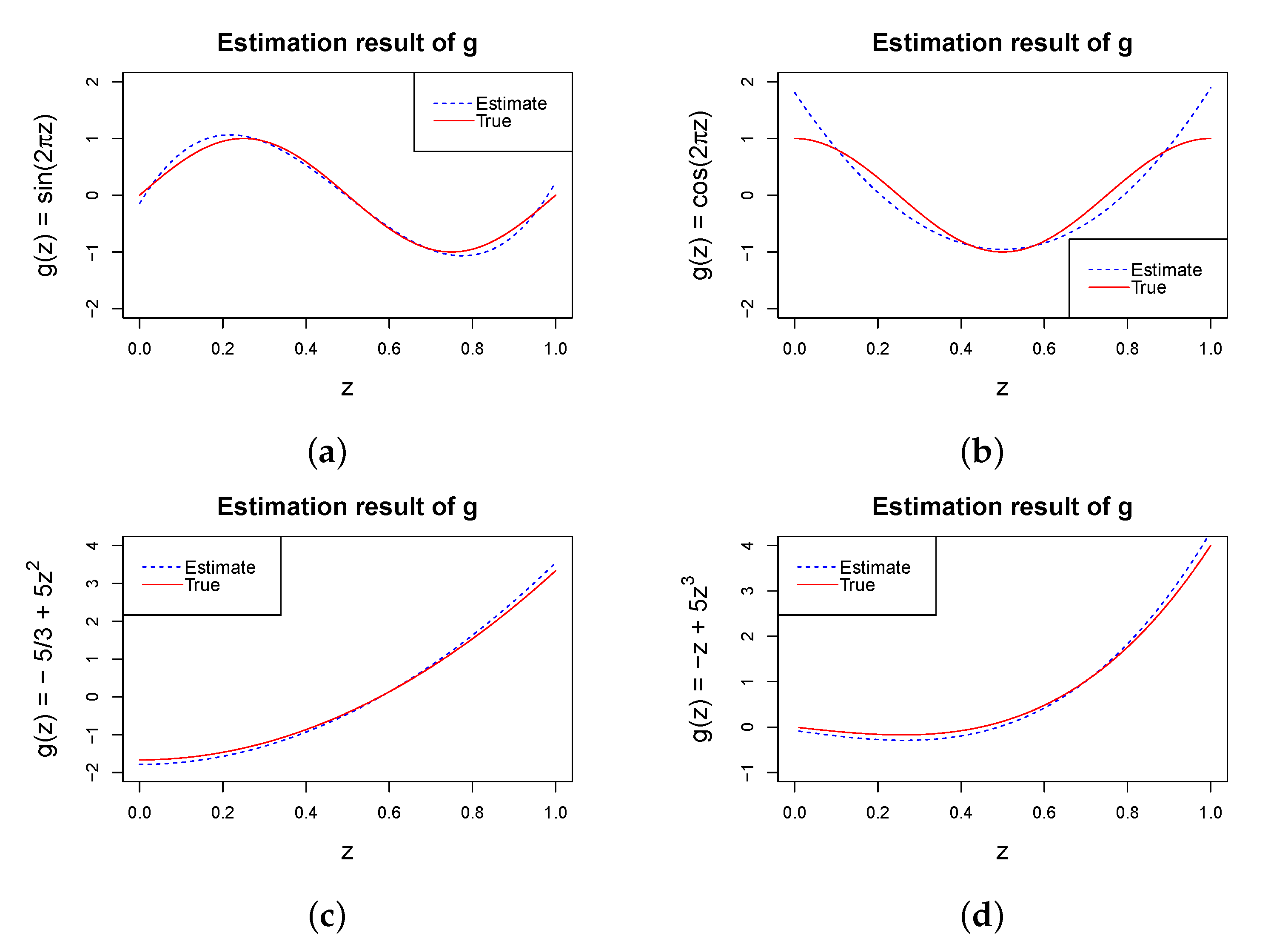
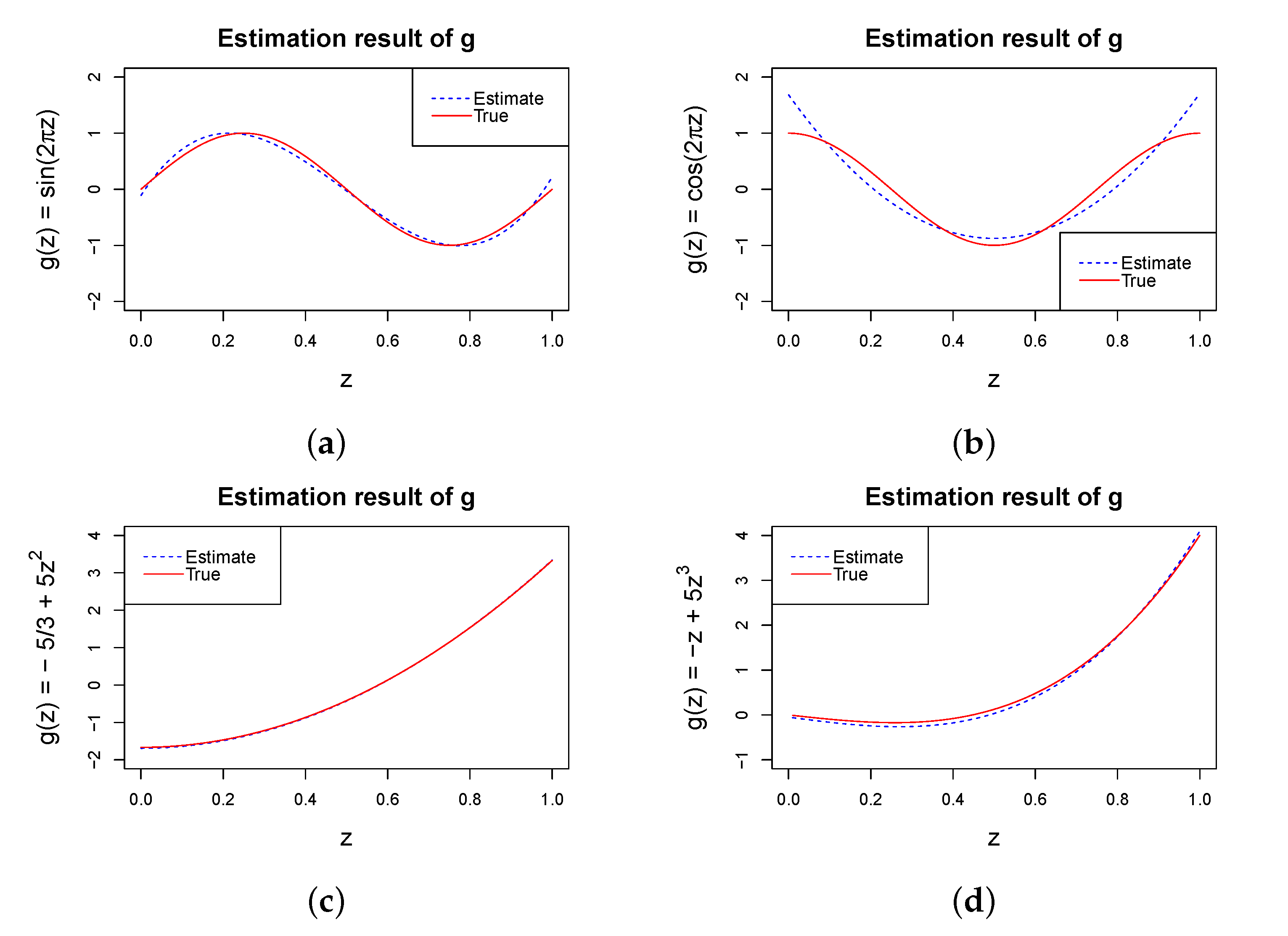
To assess the performance of the proposed method on the estimation of the nonlinear function g, we repeated the study given in Table 1 with four different g functions, $g_1(z)=sin(2\pi z)$, $g_2(z)=cos(2\pi z)$, $g_3(z)=-\frac{5}{3}+5z^2$, and $g_4(z)=-z+5z^3$, and $n=200$. Figure 1 and Figure 2 show the average of the estimated g for each of the four cases with $\beta =0$ and $\tau =0.3$ or $\tau =0.6$, respectively. The solid red lines represent the genuine functions, while the dashed blue lines represent the estimations. They show that the proposed method based on Bernstein polynomials seemed to perform reasonably well for the different Kendall’s $\tau$ considered, including a weak or strong dependency. We also took into account various configurations and got comparable outcomes.

Figure 1. Estimated g with $\beta =0$ and $\tau =0.3$; the solid red lines represent the real functions and the dashed blue lines show the estimated functions. (a) $g(z)=sin(2\pi z)$; (b) $g(z)=cos(2\pi z)$; (c) $g(z)=\frac{5}{3}-5z^2$; (d) $g(z)=-z+5z^3$.

Figure 2. Estimated g with $\beta =0$ and $\tau =0.6$; the solid red lines represent the real functions and the dashed blue lines show the estimated functions. (a) $g(z)=sin(2\pi z)$; (b) $g(z)=cos(2\pi z)$; (c) $g(z)=\frac{5}{3}-5z^2$; (d) $g(z)=-z+5z^3$.

5. An Illustration

In this section, we illustrate the proposed procedure by using the data from the Age-related Eye Disease Study (AREDS) [30], a clinical experiment tracking the development of a bilateral eye disease, age-related macular degeneration (AMD), provided the CopulaCenR package in version 4.2.0 of R software [31]. Each participant in the research was monitored every six months (during the first six years) or once a year (after year 6) for about 12 years. At each appointment, each participant’s eyes were given a severity score on a range of 1 to 12 (a higher number signifying a more serious condition).Moreover, the time-to-late AMD, which is the interval between the baseline visit and the first appointment at which the severity score reached nine or above, was computed for each eye of these subjects. Either interval censoring or right censoring was applied to the observations at both periods.

The data set consisted of $n=629$ subjects and in the analysis below, we focused on the effects of two covariates, SevScaleBL for the baseline AMD severity score (a value between one and eight with a higher value indicating more severe AMD) and rs2284665 for a genetic variant (zero, one and two for GG, GT and TT) of the AMD progression. In order to use the proposed method, we set rs2284665 to be X and SevScaleBL to be Z since the latter could be viewed as continuous. For the identifiability of the model, both X and Z were standardized and thus had the support $[0,1]$. Moreover, various degrees of Bernstein polynomials were considered, such as $m_1=m_2=3,4,5,6$.

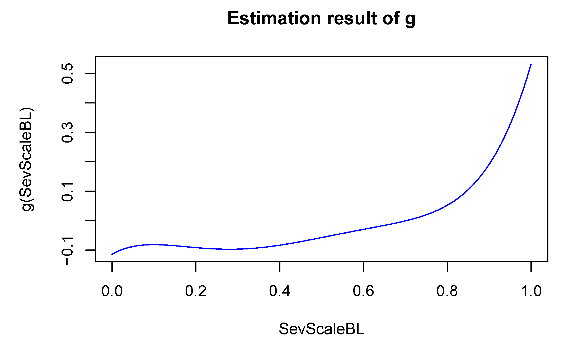
Table 5 gives the analysis results obtained by the suggested estimation approach. They include the estimated effect of the covariate rs2284665 and Kendall’s $\tau$ along with the estimated standard errors and the p-value for testing the effect to be zero. One can see that the results were consistent with respect to the degree of the Bernstein polynomials and suggested that the minor allele (TT) had a significantly “harmful” effect on AMD progression. Moreover, the estimated Kendall’s $\tau$ was $0.389$, suggesting a moderate dependence of the AMD progression between the two eyes. Figure 3 gives the estimated effect of the SevScaleBL, which indeed seemed to be nonlinear. To be more specific, the increased risk of AMD patients was associated with higher severity scores. The findings reached here were in line with those of other researchers who examined this subject [15]. It is worth pointing out that the conclusion of [15] was obtained under the proportional odds model and they could not visualize nonlinear covariate effects as in Figure 3.

Table 5. Analysis results for the AREDS data.

	$\mathit{\beta }$			$\mathit{\tau }$
Bernstein Polynomials	EST	ESE	p-Value	EST	ESE
$m_1=3,m_2=3$	0.041	0.009	<0.000	0.473	0.043
$m_1=4,m_2=4$	0.046	0.008	<0.000	0.416	0.056
$m_1=5,m_2=5$	0.034	0.008	<0.000	0.389	0.048
$m_1=6,m_2=6$	0.024	0.009	0.011	0.388	0.056

Figure 3. Estimated nonlinear effect of SevScaleBL for the illustration.

6. Concluding Remarks

In the preceding sections, the regression analysis of bivariate interval-censored survival data was considered under a family of copula-based, semiparametric, partly linear additive hazards models. As discussed above, one significant advantage of the models was that they only needed to handle the two marginal distributions via a copula function with the copula parameter determining the dependence. For inference, a sieve maximum likelihood estimation procedure with the use of Bernstein polynomials were provided, and it was shown that the resulting estimators of the regression parameters were consistent and asymptotically efficient. Furthermore, the simulation studies suggested that the recommended approach worked effectively in practical situations.

It is worth emphasizing that the main reason for using Bernstein polynomials to approximate the infinite-dimensional cumulative hazard function ${\mathsf{\Lambda }}_j(t)$ and nonlinear covariate effects $g(·)$ was its simplicity. Other smoothing functions, such as spline functions [20], could also be used, and estimation procedures similar to the one described above could be developed. In order to implement the approach, we needed to choose the degrees $m_1$ and $m_2$. As discussed above, a common method is to consider different values and compare the resulting estimators. Certainly, developing a data-driven approach for their selections would also be helpful.

In this paper, we focused on the additive hazards model. Other models, for example, the proportional hazards model, are sometimes more popular. It is well-known that the latter is more suitable for the situation where one is interested in the hazard ratio, whereas the former fits better if the excess risk or the risk differential is what is most important. However, there seems to be little literature on how to choose the better model or develop some model-checking methods, which is attractive research for the future.

References

- Sun, J. The Statistical Analysis of Interval-Censored Failure Time Data; Springer: Berlin/Heidelberg, Germany, 2006. [Google Scholar]
- Lin, D.Y.; Oakes, D.; Ying, Z. Additive hazards regression with current status data. Biometrika 1998, 85, 289–298. [Google Scholar] [CrossRef]
- Martinussen, T.; Scheike, T.H. Efficient estimation in additive hazards regression with current status data. Biometrika 2002, 89, 649–658. [Google Scholar] [CrossRef]
- Feng, Y.; Sun, J.; Sun, L. Estimation of the additive hazards model with linear inequality restrictions based on current status data. Commun. Stat.-Theory Methods 2022, 51, 68–81. [Google Scholar] [CrossRef]
- Wang, P.; Zhou, Y.; Sun, J. A new method for regression analysis of interval-censored data with the additive hazards model. J. Korean Stat. Soc. 2020, 49, 1131–1147. [Google Scholar] [CrossRef]
- Li, H.; Zhang, H.; Zhu, L.; Li, N.; Sun, J. Estimation of the additive hazards model with interval-censored data and missing covariates. Can. J. Stat. 2020, 48, 499–517. [Google Scholar] [CrossRef]
- Wang, T.B.; Yopadhyay, D.; Sinha, S. Efficient estimation of the additive risks model for interval-censored data. arXiv 2022, arXiv:2203.09726. [Google Scholar]
- Tong, X.; Chen, M.H.; Sun, J. Regression analysis of multivariate interval-censored failure time data with application to tumorigenicity experiments. Biom. J. 2008, 50, 364–374. [Google Scholar] [CrossRef] [PubMed]
- Yin, G.; Cai, J. Additive hazards model with multivariate failure time data. Biometrika 2004, 91, 801–818. [Google Scholar] [CrossRef]
- Liu, P.; Song, S.; Zhou, Y. Semiparametric additive frailty hazard model for clustered failure time data. Can. J. Stat. 2022, 50, 549–571. [Google Scholar] [CrossRef]
- Zeng, D.; Cai, J. Additive transformation models for clustered failure time data. Lifetime Data Anal. 2010, 16, 333–352. [Google Scholar] [CrossRef]
- Yu, M.; Du, M. Regression analysis of multivariate interval-censored failure time data under transformation model with informative censoring. Mathematics 2022, 10, 3257. [Google Scholar] [CrossRef]
- Sun, T.; Ding, Y. Copula-based semiparametric regression method for bivariate data under general interval censoring. Biostatistics 2021, 22, 315–330. [Google Scholar] [CrossRef]
- Marra, G.; Radice, R. Copula link-based additive models for right-censored event time data. J. Am. Stat. Assoc. 2020, 115, 886–895. [Google Scholar] [CrossRef]
- Petti, D.; Eletti, A.; Marra, G.; Radice, R. Copula link-based additive models for bivariate time-to-event outcomes with general censoring scheme. Comput. Stat. Data Anal. 2022, 175, 107550. [Google Scholar] [CrossRef]
- Cheng, G.; Zhou, L.; Huang, J.Z. Efficient semiparametric estimation in generalized partially linear additive models for longitudinal/clustered data. Bernoulli 2014, 20, 141–163. [Google Scholar] [CrossRef]
- Lu, X.; Song, P.X.K. Efficient estimation of the partly linear additive hazards model with current status data. Scand. J. Stat. 2015, 42, 306–328. [Google Scholar] [CrossRef]
- Wang, X.; Song, Y.; Zhang, S. An efficient estimation for the parameter in additive partially linear models with missing covariates. J. Korean Stat. Soc. 2020, 49, 779–801. [Google Scholar] [CrossRef]
- Lee, C.Y.; Wong, K.Y.; Lam, K.F.; Xu, J. Analysis of clustered interval-censored data using a class of semiparametric partly linear frailty transformation models. Biometrics 2022, 78, 165–178. [Google Scholar] [CrossRef] [PubMed]
- Chen, W.; Ren, F. Partially linear additive hazards regression for clustered and right censored data. Bulletin of Informatics and Cybernetics 2022, 54, 1–14. [Google Scholar] [CrossRef]
- Sklar, M. Fonctions de repartition an dimensions et leurs marges. Publ. Inst. Stat. Univ. Paris 1959, 8, 229–231. [Google Scholar]
- Nelson, R.B. An Introduction to Copulas; Springer Science and Business Media: Berlin/Heidelberg, Germany, 2006. [Google Scholar]
- Joe, H. Multivariate Models and Dependence Concepts; CRC Press: Boca Raton, FL, USA, 1997. [Google Scholar]
- Clayton, D.G. A model for association in bivariate life tables and its application in epidemiological studies of familial tendency in chronic disease incidence. Biometrika 1978, 65, 141–151. [Google Scholar] [CrossRef]
- Gumble, E.J. Bivariate exponential distributions. J. Am. Statitical Assoc. 1960, 55, 698–707. [Google Scholar] [CrossRef]
- Zhou, Q.; Hu, T.; Sun, J. A sieve semiparametric maximum likelihood approach for regression analysis of bivariate interval-censored failure time data. J. Am. Stat. Assoc. 2017, 112, 664–672. [Google Scholar] [CrossRef]
- Carnicer, J.M.; Pen˜a, J.M. Shape preserving representations and optimality of the bernstein basis. Adv. Comput. Math. 1993, 1, 173–196. [Google Scholar] [CrossRef]
- Burnham, K.P.; Anderson, D.R.; Burnham, K.P.; Anderson, D.R. Practical Use of the Information-Theoretic Approach; Springer: Berlin/Heidelberg, Germany, 1993; pp. 75–117. [Google Scholar]
- Efron, B. Bootstrap methods: Another look at the jackknife. Ann. Stat. 1979, 7, 1–26. [Google Scholar] [CrossRef]
- Age-Related Eye Disease Study Research Group. The age-related eye disease study (AREDS): Design implications AREDS report no. 1. Control. Clin. Trials 1999, 20, 573. [Google Scholar] [CrossRef]
- Sun, T.; Ding, Y. CopulaCenR: Copula based regression models for bivariate censored data in R. R J. 2020, 12, 266. [Google Scholar] [CrossRef]
- Huang, J. Efficient estimation for the proportional hazards model with interval censoring. Ann. Stat. 1996, 24, 540–568. [Google Scholar] [CrossRef]
- Zhang, Y.; Hua, L.; Huang, J. A spline-based semiparametric maximum likelihood estimation method for the cox model with interval-censored data. Scand. J. Stat. 2010, 37, 338–354. [Google Scholar] [CrossRef]
- Huang, J.; Rossini, A. Sieve estimation for the proportional-odds failure-time regression model with interval censoring. J. Am. Stat. Assoc. 1997, 92, 960–967. [Google Scholar] [CrossRef]
- Wen, C.C.; Chen, Y.H. A frailty model approach for regression analysis of bivariate interval-censored survival data. Stat. Sin. 2013, 23, 383–408. [Google Scholar] [CrossRef]
- Van der Vaart, A.; Wellner, J. Weak Convergence and Empirical Processes; Springer: Berlin/Heidelberg, Germany, 1996. [Google Scholar]
- Shen, X.; Wong, W.H. Convergence rate of sieve estimates. Ann. Stat. 1994, 22, 580–615. [Google Scholar] [CrossRef]
- Lorentz, G.G. Bernstein Polynomials; American Mathematical Society: Providence, RI, USA, 2013. [Google Scholar]
Disclaimer/Publisher’s Note: The statements, opinions and data contained in all publications are solely those of the individual author(s) and contributor(s) and not of MDPI and/or the editor(s). MDPI and/or the editor(s) disclaim responsibility for any injury to people or property resulting from any ideas, methods, instructions or products referred to in the content. |
© 2023 by the authors. Licensee MDPI, Basel, Switzerland. This article is an open access article distributed under the terms and conditions of the Creative Commons Attribution (CC BY) license (https://creativecommons.org/licenses/by/4.0/).