Generalized Partially Functional Linear Model with Unknown Link Function

Abstract

In existing models with an unknown link function, the issue of predictors containing both multiple functional data and multiple scalar data has not been studied. To fill this gap, we propose a generalized partially functional linear model, which not only models the relationship between multiple scalar and functional predictors and responses, but also automatically estimates the link function. Specifically, we use the functional principal component analysis method to reduce the dimensionality of functional predictors, estimate the regression coefficients using the maximum likelihood estimation method, estimate the link function using the method of local linear regression, iteratively obtain the final estimator, and establish the asymptotic normality of the estimator. The asymptotic normality is illustrated through simulation experiments. Finally, the proposed model is applied to study the influence of environmental, economic, and medical levels on life expectancy in China. In the study, functional predictors are the daily air quality index, temperature, and humidity of 58 cities in 2020, and scalar predictors are GDP and the number of beds in hospitals. The experimental results indicate that the unknown link function model has a smaller prediction error and better performance than both the model with the known link function and the model without a link function.

1. Introduction

In 1982, Ramsay [1] first proposed the definition of functional data, laying a foundation for the development of functional data analysis. In 2005, Ramsay and Silverman provided a detailed introduction to the general methods and steps of functional data analysis, including functional principal component analysis and functional linear regression models in their book [2]. In 2012, Horváth and Kokoszka [3] focused on the inferential methods in functional data analysis.

In 2009, Shin [4] proposed a partial functional linear model (PFLM), which explores the relationship between a scalar response variable and mixed-type predictors. In 2012, Shin and Lee [5] derived the asymptotic prediction rate of PFLM and compared it with that of other functional regression models.

In 2002, James [6] proposed generalized linear models with functional predictors and applied them to standard missing data problems. In 2005, Müller and Stadtmüller [7] proposed a generalized functional linear regression model where the response variable is a scalar and the predictor is a random function. They also considered the situation where the link and variance functions were unknown. In 2015, Shang and Cheng [8] proposed a roughness regularization approach in making nonparametric inference for generalized functional linear models with known link functions. In 2019, Wong et al. [9] investigated a class of partially linear functional additive models that predict a scalar response by both the parametric effects of a multivariate predictor and the non-parametric effects of a multivariate functional predictor.

In a generalized linear model, sometimes the link function may not be known exactly, but can be assumed to be of some general ‘parametric’ form. In 1984, Scallan et al. [10] showed how generalized linear models can be extended to fit models with such link functions.

In 1994, Weisberg and Welsh [11] used kernel smoothing estimation to estimate the link function and estimated regression coefficients through the link function, then alternated between these two steps, which effectively solves the fitting problem when the link function is unknown. However, kernel smoothing estimation may have problems at the boundary, so local polynomial fitting is introduced, which performs better near the boundary.

In 1998, Chiou and Müller [12] considered the condition of the link and the variance functions to be unknown but smooth. Consistency results for the link and the variance function estimators, as well as the sampling distribution of the regression coefficients, were obtained. In 2005, Chiou and Müller [13] introduced a flexible marginal modeling approach for statistical inference for clustered and longitudinal data under minimal assumptions. The predictor was longitudinal data in the model. The estimated estimating equation approach was semi-parametric. The semi-parametric model proposed was fitted by quasi-likelihood regression. The consistency of the estimates of the link and variance functions and the asymptotic limit distribution of regression coefficients were given. In addition, there are other methods to estimate unknown functions. In 2009, Bai et al. [14] focused on single-index models for longitudinal data. They proposed a procedure to estimate the single-index component and the unknown link function based on the combination of the penalized splines and quadratic inference functions. In 2012, Pang and Xue [15] generalized the single-index models to the scenarios with random effects. The link function was estimated by using the local linear smoother. A new set of estimating equations modified for the boundary effects was proposed to estimate the index coefficients. In 2017, Yuan and Diao [16] developed a sieve maximum likelihood estimation for generalized linear models, in which the estimator of the unknown link function was assumed to lie in a sieve space. Various methods of sieves including the B-spline and P-spline-based methods were introduced.

In 2017, Kokoszka and Reimherr [17] wrote a book that introduced the basic concepts, methods, and applications of functional data analysis. The book provided a clear and systematic overview, covering key areas such as representation, smoothing, interpolation, statistical modeling, and inference for functional data. It also included detailed explanations of practical examples and computational methods. In 2023, Rao and Reimherr [18] introduced a novel neural network-based nonlinear model of functional data designed to exploit the structure of functional data and fit it with a derived function gradient optimization algorithm, demonstrating the effectiveness of these methods in dealing with complex functional models and providing new breakthroughs for deep learning applications in the field of functional data analysis.

The relationship between environmental factors and human health has been a topic of significant research interest in recent years. In 2012, Huang et al. [19] explored the relationship between temperature and years of life lost (YLL). The study found that both high and low temperatures lead to an increase in YLL, with high temperatures having a greater impact. In 2020, Yang et al. [20] applied a generalized additive model to assess the associations between daily PM2.5 exposure and YLL due to respiratory diseases in 96 Chinese cities during 2013–2016. They further estimated the avoidable YLL and potential gains in life expectancy under the assumption that daily PM2.5 level met World Health Organization standards. In 2021, Deryugina and Molitor [21] explored the factors influencing life expectancy across the United States. The study found that individuals living in areas with severe air pollution, poor water quality, and inadequate healthcare facilities generally had shorter life expectancy and poorer health conditions.

In summary, the existing models with unknown link functions have not addressed the issue of the generalized partially functional regression model, which involves regressing the response variable on multiple functional and scalar predictors. To fill this gap, this study proposes a generalized partially functional linear model with an unknown link function. The proposed model avoids the problem of decreased model accuracy caused by selecting an incorrect link function. The predictors in the proposed model include both multiple functional data and multiple scalar data. It reveals the complex relationships between variables and provides a flexible and effective modeling approach. It can achieve better prediction and explanation.

The paper is organized as follows. All the published works and definitions that are referred to in the process of theorem proving are introduced in Section 2. The abbreviations used in the article are introduced in the Section 3.1. The generalized partial functional linear model with unknown link function is proposed in Section 3.2. The estimation of the regression coefficients and the link function is discussed in Section 3.3. In Section 4, asymptotic normality of estimators are derived. Simulation results are reported in Section 5. The average life expectancy study in 58 cities in China is given in Section 6. In Section 7, a brief summary and limitations of the research are provided. Possible applications and future directions are presented in Section 7.

2. Preliminaries

In this section, we provide an overview of the published works and definitions that are relevant to our research. These preliminary concepts and references lay the foundation for a better understanding of the subsequent discussion.

(1) In 1982, Mack and Silverman [22] provided a comprehensive analysis of the weak and strong uniform consistency properties of kernel regression estimates, highlighted their theoretical properties and practical significance in non-parametric regression modeling. In this paper, we directly apply the results of Proposition 4 as Lemma 1 for Theorem 1 in this paper.

(2) In 1995, Masry and Tjøstheim [23] discussed the estimation and identification of nonlinear time series of ARCH type. They provided an estimation method to obtain consistent estimates of the parameters and proved the asymptotic normality. They also explored model identification methods. Their studies are of significant importance for modeling and analyzing financial time series. Theorem 3.3 in their work is used to prove Theorem 1 in this paper.

(3) In 1999, Chiou and Müller [24] focused on the study of non-parametric quasi-likelihood methods. They provided the theoretical derivation process of this method, and explored its applications in statistical inference. Theorem 4.1 in their paper is used to prove Lemma 2 and Lemma 3 for Theorem 2 in this paper.

(4) In 2021, Xiao et al. [25] proposed a generalized partially functional linear regression model where the response variable is 0 or 1 and the predictors were multiple functional and scalar, and the asymptotic property of the estimated coefficients in the model was established. The proof method of Theorem 1 in [25] is used to prove Theorem 2 in this work.

3. Model and Estimation

The data we observe for the i-th subject are $\{Y_i,X_{i1}\left(t\right),X_{i2}\left(t\right),\cdots ,X_{id}\left(t\right),Z_i\},$ $i=1,\dots ,n.$ We assume that these data are independent, identically distributed (i.i.d) copies of $\{Y,X_1\left(t\right),\cdots ,X_d\left(t\right),Z\}$. For $j=1,\cdots ,d,$ the functional predictor $X_j\left(t\right)$ is a random curve. $X_{ij}\left(t\right),i=1,2,\cdots ,n$ are samples of $X_j\left(t\right)$ and $X_{ij}\left(t\right)$ are square integrable on a real bounded interval T, i.e., $X_{ij}\left(t\right)\in L^2\left(T\right)$. $L^2\left(T\right)$ refers to the space of square integrable functions defined on T. And the scalar predictor vector $Z={(Z_1,Z_2,\dots ,Z_q)}^T$ is a q dimensional random vector. The response Y is a real-valued random variable that may be binary or count.

3.1. Abbreviation Introduction

Table 1 is a list of the abbreviations we use in this work along with their corresponding full forms:

Table 1. The abbreviations and their corresponding full forms.

Abbreviation	Full Form
FPCA	Functional principal component analysis
KL expansion	Karhunen–Loeve expansion
RMISE	Root Mean Integrated Square Error
SD	Standard Deviation
GCV	Generalized Cross Validation
MAE	Mean Absolute Error
MSE	Mean Squared Error
TP	True Positive
TN	True Negative
FP	False Positive
FN	False Negative

3.2. Model

We establish a model for the relationship between the response variable $Y_i$ and the predictors $X_{ij}\left(t\right),j=1,2,\cdots ,d$ and $Z_i$:

$$Y_i=g(\sum _{j=1}^d{\int }_T{X}_{ij}\left(t\right){\beta }_j\left(t\right)dt+{Z_i}^T\gamma )+{\epsilon }_i,$$

(1)

where ${\beta }_j(·)$ is the regression coefficient function that needs to be estimated for the functional predictors $X_{ij}\left(t\right)$; $\gamma$ is a q dimensional vector with the elements to be the regression coefficients for the scalar predictors $Z_i$ that need to be estimated, i.e., $\gamma ={({\gamma }_1,{\gamma }_2,\dots ,{\gamma }_q)}^T$. Here ${\epsilon }_i$ is i.i.d copies of $\epsilon$, which is the random error variable and $\epsilon =Y-g\left(\eta \right)$, $E\left[\epsilon \left|X_j\left(t\right),Z\right.\right]=0$, where

$$\eta =\sum _{j=1}^d{\int }_T{X}_j\left(t\right){\beta }_j\left(t\right)dt+Z^T\gamma .$$

The relationship between the response variable Y and $\eta$ is established through $g(·)$, i.e., $E\left[Y\right|X_j\left(T\right),Z]=\mu =g\left(\eta \right)$. $g(·)$ is the link function that is unknown and needs to be estimated in this paper.

Let ${\sigma }^2(·)$ be a variance function that satisfies ${\sigma }^2(·)\ge c>0$ for a constant $c>0$, such that

$$Var\left[Y\right|X_j\left(t\right),Z]={\sigma }^2\left(\mu \right)={\sigma }^2\left(g\left(\eta \right)\right),$$

$$Var\left[\epsilon \right]=E\left[{\epsilon }^2\right]={\sigma }^2\left(E\left[Y\right|X_j\left(t\right),Z]\right).$$

To reduce the dimensionality of the functional predictors $X_{ij}\left(t\right)$, we adopt the method of FPCA in this paper. First, we need to standardize the original data by centering them, so that $E\left[X_{ij}\left(t\right)\right]=0,j=1,\cdots ,d,$ and $E\left[Z_l\right]=0,l=1,\cdots ,q$.

By KL expansion and Mercer’s theorem, $X_{ij}\left(t\right)$ can be expanded as

$$X_{ij}\left(t\right)=\sum _{k=1}^{\infty }{\xi }_{ijk}{\rho }_{jk}\left(t\right),$$

(2)

where ${\xi }_{ijk}$ represents the functional principal component scores, and ${\rho }_{jk}(·)$ are called functional principal components, which are the eigenfunctions of the covariance operator of $X_{ij}\left(t\right)$. Notice that ${\rho }_{jk}(·),k=1,2,\cdots$ form an orthonormal basis for the function space $L^2\left(T\right)$. Then regression coefficient function ${\beta }_j\left(t\right)\in L^2\left(T\right)$ can be expanded as

$${\beta }_j\left(t\right)=\sum _{k=1}^{\infty }{\chi }_{jk}{\rho }_{jk}\left(t\right).$$

(3)

where ${\chi }_{jk}$ represents the functional principal component scores.

After plugging the above two expansions into (1), we have

$$Y_i=g\left(\sum _{j=1}^d\sum _{k=1}^{m_j}{\xi }_{ijk}{\chi }_{jk}+{Z_i}^T\gamma \right)+{\epsilon }_i.$$

(4)

In (4), we truncated the predictors at $m_j$ (depending on sample size n), and $m_j$ increases asymptotically with $n\to \infty$.

3.3. Estimation

Define a parameter vector ${\theta }_0$, where

$${\theta }_0={({\chi }_{11},{\chi }_{12},\cdots ,{\chi }_{1m_1},\cdots ,{\chi }_{d1},{\chi }_{d2},\cdots ,{\chi }_{d{m}_d},{\gamma }_1,\cdots ,{\gamma }_q)}^T.$$

For the estimation of the parameter vector $\theta$ and the link function g, we use an iterative estimation method to obtain the final estimates. Let there exist a constant $c>0$; with this c and n, we can define ${\theta }_n=\{\theta :∥\theta -{\theta }_0∥\le c{n}^{-1/\phantom{-12}2}\}$. The norm of finite dimensional spaces used in this paper is the Euclidean norm. The overall iterative process is briefly described below:

Step 1 To obtain the estimate ${\theta }^{\left(0\right)}$ of ${\theta }_0$ by solving Equation (5), it is assumed that the link function $g(·)$ is known. The link function $g(·)$ is required to be second-order continuously differentiable to ensure the existence of the Hessian matrix, moreover, for the variance function ${\sigma }^2(·)$ is defined on the range of link function and is strictly positive.

$$U\left(\theta \right)=\sum _{i=1}^n(Y_i-{\mu }_i)\frac{g^{\prime }\left({\eta }_i\right)}{{\sigma }^2\left({\mu }_i\right)}{\Delta }_i=0,$$

(5)

where ${\eta }_i={\displaystyle \sum _{j=1}^d}{\displaystyle \sum _{k=1}^{m_j}}{\xi }_{ijk}{\tilde{\chi }}_{jk}+Z_i\tilde{\gamma }$, $\tilde{\chi }$ near $\chi$, $\tilde{\gamma }$ near $\gamma$, ${\mu }_i=g\left({\eta }_i\right)$ and

$${\Delta }_i={({\xi }_{i11},{\xi }_{i12},\cdots ,{\xi }_{i1m_1},\cdots ,{\xi }_{id1},{\xi }_{id2},\cdots ,{\xi }_{id{m}_d},z_{i1},\cdots ,z_{iq})}^T.$$

Here, $\tilde{\chi }$ and $\tilde{\gamma }$ represent the corresponding estimated value in step 1 but not the final estimate.

We introduce the following matrix:

$$D_0=D_{n,q}={\left(z_{il}\right)}_{1\le i\le n,1\le l\le q},$$

$$D_j=D_{n,m_j}={\left({\xi }_{ijk}\right)}_{1\le i\le n,1\le j\le d,1\le k\le m_j},$$

$$D=D_{n,q+{\sum }_{j=1}^d{m}_j}=\left(D_0,D_1,\dots ,D_d\right),$$

$$V=diag\left({\sigma }^2\left({\mu }_1\right),{\sigma }^2\left({\mu }_2\right),\dots ,{\sigma }^2\left({\mu }_n\right)\right),$$

$$G=diag{\left(g^{\prime }\left({\eta }_i\right)\right)}_{1\le i\le n},$$

$$Y={\left(Y_1,Y_2,\dots ,Y_n\right)}^T,$$

$$\mu ={\left({\mu }_1,{\mu }_2,\dots ,{\mu }_n\right)}^T.$$

Then, Equation (5) can be expressed in matrix form, i.e.,

$$D^T{V}^{-1}G\left(Y-\mu \right)=0.$$

We can solve it by the weighted least squares method. A Taylor expansion of $g^{-1}\left(Y\right)$, where

$$\begin{array}{cc}\hfill g^{-1}\left(Y\right)& =g^{-1}\left(\mu \right)+{\left[g^{-1}\left(\mu \right)\right]}^{\prime }(Y-\mu )\hfill \\ \hfill & =\eta +G^{-1}(Y-\mu ),\hfill \end{array}$$

and then we can get

$$D^{T}W\left(g^{-1}\left(Y\right)-\eta \right)=0,$$

where $W=V^{-1}{G}^2$. Simplification yields estimates

$${\tilde{\chi }}_j^{\left(0\right)}={\left(D_j^{T}W{D}_j\right)}^{-1}{D}_j^{T}W{g}^{-1}\left(Y\right),$$

$${\tilde{\gamma }}_j^{\left(0\right)}={\left(D_0^{T}W{D}_0\right)}^{-1}{D}_0^{T}W{g}^{-1}\left(Y\right),$$

where ${\tilde{\chi }}_j^{\left(0\right)}={({\tilde{\chi }}_{j1}^{\left(0\right)},\cdots ,{\tilde{\chi }}_{jm}^{\left(0\right)})}^T,j=1,2,\cdots ,d$, ${\tilde{\gamma }}^{\left(0\right)}={({\tilde{\gamma }}_1^{\left(0\right)},{\tilde{\gamma }}_2^{\left(0\right)},\cdots ,{\tilde{\gamma }}_q^{\left(0\right)})}^T$.

Let

$${\tilde{\theta }}^{\left(0\right)}={({\tilde{\chi }}_{11}^{\left(0\right)},{\tilde{\chi }}_{12}^{\left(0\right)},\cdots ,{\tilde{\chi }}_{1m_1}^{\left(0\right)},\cdots ,{\tilde{\chi }}_{d1}^{\left(0\right)},{\tilde{\chi }}_{d2}^{\left(0\right)},\cdots ,{\tilde{\chi }}_{d{m}_d}^{\left(0\right)},{\tilde{\gamma }}_1^{\left(0\right)},{\tilde{\gamma }}_2^{\left(0\right)},\cdots ,{\tilde{\gamma }}_q^{\left(0\right)})}^T.$$

Step 2 By local linear regression, the estimates $g^{\left(0\right)}$, $g^{\prime \left(0\right)}$ of the link functions g, $g^{\prime }$ are obtained.

Let the bandwidth $b=b_n$ of the kernel function $k(·)$ converge to zero and define $k_b(·)=b^{-1}k\left(·/\phantom{·b}b\right)$. Since the convergence rates of $g(·)$ and $g^{\prime }(·)$ are different, their bandwidth choices should also be different. Let $h_0=h_{0n}$ denote the bandwidth of $g(·)$, and $h_1=h_{1n}$ denote the bandwidth of $g^{\prime }(·)$, but in this paper, for simplicity, the bandwidth $h=h_0=h_1$ is chosen. Let the distributions of both the functional predictors $X_j\left(t\right)$ and the scalar predictors Z belong to a compact support set U, and we have $\mathsf{\Omega }=\{u={\eta }_i\left|X_j\left(t\right),Z\in U\right.\}$. To simplify the expression, we let $g=g(u;\theta )$, $g^{\prime }=g^{\prime }(u;\theta )$. For a fixed $\theta$, apply the method of local linear regression to obtain an initial estimate of ${\tilde{g}}^{\left(0\right)}$ and ${\tilde{g}}^{\prime \left(0\right)}$ for g and $g^{\prime }$, respectively. We minimize the weighted sum of squares at any point u, and the formula for calculating the weighted sum of squares is

$$\sum _{i=1}^n{[Y_i-g-g^{\prime }({\eta }_i-u)]}^2{k}_h({\eta }_i-u).$$

(6)

Through minimizing (6), we can obtain ${\tilde{g}}^{\left(0\right)}$ and ${\tilde{g}}^{\prime \left(0\right)}$, and they can be represented as ${\tilde{g}}^{\left(0\right)}={\displaystyle \sum _{i=1}^n}{\omega }_i(u;\theta )Y_i$, ${\tilde{g}}^{\prime \left(0\right)}={\displaystyle \sum _{i=1}^n}{\tilde{\omega }}_i(u;\theta )Y_i$, where

$${\omega }_i(u;\theta )=\frac{k_h({\eta }_i-u)[{\phi }_{n,2}(u;\theta ,h)-({\eta }_i-u){\phi }_{n,1}(u;\theta ,h)]}{{\phi }_{n,0}(u;\theta ,h){\phi }_{n,2}(u;\theta ,h)-{\phi }_{n,1}^2(u;\theta ,h)},$$

$${\tilde{\omega }}_i(u;\theta )=\frac{k_h({\eta }_i-u)[({\eta }_i-u){\phi }_{n,0}(u;\theta ,h)-{\phi }_{n,1}(u;\theta ,h)]}{{\phi }_{n,0}(u;\theta ,h){\phi }_{n,2}(u;\theta ,h)-{\phi }_{n,1}^2(u;\theta ,h)},$$

$${\phi }_{n,l}(u;\theta ,h)=\frac{1}{n}\sum _{i=1}^n{\left(\frac{{\eta }_i-u}{h}\right)}^l{k}_h({\eta }_i-u),l=0,1,2.$$

Step 3 Using the method of Step 1, the link function is replaced by the estimated link functions ${\tilde{g}}^{\left(\alpha \right)}$ and ${\tilde{g}}^{\prime \left(\alpha \right)}$, where $\alpha =0,1,2,\dots$. To update ${\tilde{\theta }}^{\left(\alpha \right)}$, solve the estimation equation (5) for $\theta$. From this we can obtain the estimated value of ${\tilde{\theta }}^{\left(\alpha \right)}$

$${\tilde{\theta }}^{\left(\alpha \right)}={({\tilde{\chi }}_{11}^{\left(\alpha \right)},{\tilde{\chi }}_{12}^{\left(\alpha \right)},\cdots ,{\tilde{\chi }}_{1m_1}^{\left(\alpha \right)},\cdots ,{\tilde{\chi }}_{d1}^{\left(\alpha \right)},{\tilde{\chi }}_{d2}^{\left(\alpha \right)},\cdots ,{\tilde{\chi }}_{d{m}_d}^{\left(\alpha \right)},{\tilde{\gamma }}_1^{\left(\alpha \right)},{\tilde{\gamma }}_2^{\left(\alpha \right)},\cdots ,{\tilde{\gamma }}_q^{\left(\alpha \right)})}^T.$$

Step 4 Using the method in Step 2, the parameter vector is replaced by the estimated ${\tilde{\theta }}^{\left(\alpha \right)}={({\tilde{\chi }}_{j1}^{\left(\alpha \right)},{\tilde{\chi }}_{j2}^{\left(\alpha \right)},\cdots ,{\tilde{\chi }}_{jm}^{\left(\alpha \right)},{\tilde{\gamma }}_1^{\left(\alpha \right)},{\tilde{\gamma }}_2^{\left(\alpha \right)},\cdots ,{\tilde{\gamma }}_q^{\left(\alpha \right)})}^T$, where $\alpha =1,2,3,\dots$ From this we obtain the estimates ${\tilde{g}}^{\left(\alpha \right)}$ and ${\tilde{g}}^{\prime \left(\alpha \right)}$ for g and $g^{\prime }$, where $\alpha =1,2,3,\dots$

Step 5 Repeat the above steps until $\left|{\tilde{\theta }}^{(\alpha +1)}-{\tilde{\theta }}^{\left(\alpha \right)}\right|$ converge, and stop the iteration.

Step 6 The final estimate of the regression coefficient $\theta$ is obtained as $\widehat{\theta }$, and the estimate of the link function g is obtained as $\widehat{g}$.

4. Asymptotic Properties

To derive the asymptotics of the estimates of the link function $\widehat{g}$ and the regression coefficients $\widehat{\theta }$, some additional assumptions are required:

(C1)

There exists $b=max(4,c)$ for a constant $c>0$, such that $E\left[{\int }_T{∥X_j\left(t\right)∥}^{b}dt\right]<\infty ,j=1,\cdots ,d,E\left[{∥Z∥}^b\right]<\infty ,E\left[\epsilon \right]<\infty .$

(C2)

Let the density function $f(·)$ of ${\eta }_i$ be strictly positive, and $f(·)$ satisfies the first-order Lipschitz condition when $\theta \to {\theta }_0$.

(C3)

The kernel function $k(·)$ satisfies the first-order Lipschitz condition and is a bounded and continuous symmetric probability density function and satisfies ${\int }_{-\infty }^{\infty }{u}^{2}k\left(u\right)du\ne 0,{\int }_{-\infty }^{\infty }{\left|u\right|}^{2}k\left(u\right)du<\infty .$

(C4)

$n{h}^4/{log}^{2}n\to \infty ,n{h}^5=O\left(1\right)$. Here, h is the bandwidth of the kernel function.

(C5)

For $j=1,\cdots ,d$, $m_j{n}^{-1/4}\to 0$ as $n\to \infty$.

Remark 1. 

(C1) It is a necessary condition for the asymptotic normality of the estimator. (C2) Ensures that ${\tilde{g}}^{\left(\alpha \right)}$, ${\tilde{g}}^{\prime \left(\alpha \right)}$ are far from 0 when ${\tilde{\theta }}^{\left(\alpha \right)}$ is close enough to θ. (C3) The usual assumptions about the kernel function. (C4) The usual assumptions about the bandwidth. (C5) Some controls are applied to m in order to make the convergence faster.

4.1. Asymptotic Convergence of $g^{\left(\alpha \right)}$

Lemma 1. 

Let $({\zeta }_1,{\iota }_1),\dots ,({\zeta }_n,{\iota }_n)$ be independent and identically distributed random vectors. Furthermore, assume that for any $s>0$, there exist $E{\left|{\iota }_i\right|}^s<\infty$, $i=1,\dots ,n$ and $\underset{\zeta }{sup}\int {\left|\iota \right|}^{s}f(\zeta ,\iota )d\iota <\infty$ such that $f(·,·)$ is the joint density function of $(\zeta ,\iota )$. Let $k(·)$ be a bounded and strictly positive kernel function that satisfies the Lipschitz condition, we have

$$\underset{\zeta }{sup}\left|\frac{1}{n}\sum _{i=1}^n\left[k_h({\zeta }_i-\zeta ){\iota }_i-E\left[k_h({\zeta }_i-\zeta ){\iota }_i\right]\right]\right|=O_p\left[{\left(\frac{log\left(1/\phantom{1h}h\right)}{nh}\right)}^{\frac{1}{2}}\right].$$

Proof. 

See Proposition 4 in Mack and Silverman (1982) [22]. □

Theorem 1. 

If we assume that (C1)–(C5) holds, for ${\sigma }^2>0$, then we have

$$\sqrt{nh}[{\tilde{g}}^{\left(\alpha \right)}(u;\theta )-g\left(u\right)-I\left(u\right)]\stackrel{D}{\to }N(0,{\vartheta }^2\left(u\right))$$

where $I\left(u\right)=\frac{1}{2}{h}^2{\mu }_2{g}^{″}\left(u\right)$, ${\vartheta }^2\left(u\right)={\nu }_2{\sigma }^2/\phantom{{\nu }_2{\sigma }^2{\sum }_{j=1}^d{f}_j\left(u\right)}{\sum }_{j=1}^d{f}_j\left(u\right)$, and for the kernel function, let

$${\mu }_l=\int u^{l}k\left(u\right)du,{\nu }_l=\int k^l\left(u\right)du,l=1,2.$$

Proof. 

$${\left({\tilde{g}}^{\left(\alpha \right)}(u;{\theta }_0),h{\tilde{g}}^{\prime \left(\alpha \right)}(u;{\theta }_0)\right)}^T={\Gamma }_n^{-1}(u;{\theta }_0){\mathsf{\Phi }}_n(u;{\theta }_0),$$

(7)

where

$${\Gamma }_n(u;{\theta }_0)=\left(\begin{array}{cc}{\phi }_{n,0}(u;{\theta }_0)& {\phi }_{n,1}(u;{\theta }_0)\\ {\phi }_{n,1}(u;{\theta }_0)& {\phi }_{n,2}(u;{\theta }_0)\end{array}\right),$$

$${\mathsf{\Phi }}_n(u;{\theta }_0)={\left({\varphi }_{n,0}(u;{\theta }_0),{\varphi }_{n,1}(u;{\theta }_0)\right)}^T,$$

$${\phi }_{n,l}(u;{\theta }_0)=\frac{1}{n}\sum _{i=1}^n{\left(\frac{{\eta }_{i0}-u}{h}\right)}^l{k}_h({\eta }_{i0}-u),l=0,1,2,$$

$${\varphi }_{n,l}(u;{\theta }_0)=\frac{1}{n}\sum _{i=1}^n{Y_i\left(\frac{{\eta }_{i0}-u}{h}\right)}^l{k}_h({\eta }_{i0}-u),l=0,1,$$

$${\eta }_{i0}=\sum _{j=1}^d\sum _{k=1}^{m_j}{\xi }_{ijk}{\chi }_{jk}+{Z_i}^T\gamma .$$

By expanding ${\phi }_{n,l}(u;\theta )$, $l=0,1,2,3$, we obtain that

$$\begin{array}{cc}\hfill E\left[{\phi }_{n,l}\left(u;\theta \right)\right]& =E\left[\frac{1}{n}\sum _{i=1}^n{\left(\frac{{\eta }_i-u}{h}\right)}^l{k}_h\left({\eta }_i-u\right)\right]\hfill \\ \hfill & =\sum _{j=1}^d{f}_j\left(u\right){\mu }_l+O\left(h\right).\hfill \end{array}$$

(8)

From Lemma 1, it can be proved that for $l=0,1,2,3$

$$\begin{array}{c}\hfill {\phi }_{n,l}(u;\theta )-E\left[{\phi }_{n,l}(u;\theta )\right]=O_p\left[{\left(\frac{log\left(1/\phantom{1h}h\right)}{nh}\right)}^{\frac{1}{2}}\right].\end{array}$$

(9)

Taking (8) into (9), we can obtain that

$${\phi }_{n,l}(u;\theta )=\sum _{j=1}^d{f}_j\left(u\right){\mu }_l+O_p\left[{\left(\frac{log\left(1/\phantom{1h}h\right)}{nh}\right)}^{\frac{1}{2}}+h\right].$$

Then

$${\Gamma }_n(u;\theta )=\Gamma \left(u\right)+O_p\left[{\left(\frac{log\left(1/\phantom{1h}h\right)}{nh}\right)}^{\frac{1}{2}}+h\right],$$

where $\Gamma \left(u\right)={\displaystyle \sum _{j=1}^d}{f}_j\left(u\right)\otimes diag(1,{\mu }_2)$, ⊗ indicates the Kronecker product.

Inverting the matrix ${\Gamma }_n(u;\theta )$, we get

$${\Gamma }_n^{-1}(u;\theta )={\Gamma }^{-1}\left(u\right)+O_p\left[{\left(\frac{log\left(1/\phantom{1h}h\right)}{nh}\right)}^{\frac{1}{2}}+h\right].$$

Let

$$\begin{array}{c}\hfill {\varphi }_{n,l}^{*}(u;\theta )=\frac{1}{n}\sum _{i=1}^n{[Y_i-g\left({\eta }_i\right)]\left(\frac{{\eta }_i-u}{h}\right)}^l{k}_h({\eta }_i-u),\end{array}$$

(10)

where $l=0,1$, and

$${\mathsf{\Phi }}_n^{*}\equiv {\mathsf{\Phi }}_n^{*}(u;\theta )={\left({\varphi }_{n,0}^{*}(u;\theta ),{\varphi }_{n,1}^{*}(u;\theta )\right)}^T.$$

By expanding ${\varphi }_{n,l}^{*}(u;\theta )$, we obtain when $l=0,1,2,$

$$\begin{array}{cc}\hfill E\left[{\varphi }_{n,l}^{*}\left(u;\theta \right)\right]& =E\left[\frac{1}{n}\sum _{i=1}^n\left[Y_i-g\left({\eta }_i\right)\right]{\left(\frac{{\eta }_i-u}{h}\right)}^l{k}_h\left({\eta }_i-u\right)\right]\hfill \\ \hfill & =O\left(n^{-\frac{1}{2}}\right).\hfill \end{array}$$

(11)

From Lemma 1, combined with (10) and (11), we can prove that

$${\varphi }_{n,l}^{*}(u;\theta )=O_p\left[{\left(\frac{log\left(1/\phantom{1h}h\right)}{nh}\right)}^{\frac{1}{2}}+n^{-1/\phantom{12}2}\right].$$

The Taylor expansion of $g\left({\eta }_i\right)$ at u is

$$\begin{array}{c}\hfill {\mathsf{\Phi }}_n-{\mathsf{\Phi }}_n^{*}={\Gamma }_n\left(\begin{array}{c}g\left(u\right)\\ h{g}^{\prime }\left(u\right)\end{array}\right)+\frac{1}{2}{h}^2\left(\begin{array}{c}{\phi }_{n,2}{g}^{″}\left(u\right)\\ {\phi }_{n,3}{g}^{″}\left(u\right)\end{array}\right)+o_p\left(h^2\right),\end{array}$$

(12)

where ${\Gamma }_n={\Gamma }_n(u;\theta )$, ${\phi }_{n,l}={\phi }_{n,l}(u;\theta ),l=2,3$.

Combining (7) and (12), we can obtain

$$\begin{array}{cc}\hfill \left(\begin{array}{c}{\tilde{g}}^{\left(\alpha \right)}-g\\ h[{\tilde{g}}^{\prime \left(\alpha \right)}-g^{\prime }]\end{array}\right)& ={\Gamma }_n^{-1}{\mathsf{\Phi }}_n^{*}+\frac{1}{2}{\Gamma }_n^{-1}{h}^2\left(\begin{array}{c}{\phi }_{n,2}{g}^{″}\left(u\right)\hfill \\ {\phi }_{n,3}{g}^{″}\left(u\right)\hfill \end{array}\right)+o_p\left(h^2\right)\hfill \\ & ={\Gamma }^{-1}\left(u\right){\mathsf{\Phi }}_n^{*}+\frac{1}{2}{h}^2\left(\begin{array}{c}{\mu }_2{g}^{″}\left(u\right)\hfill \\ \frac{{\mu }_3}{{\mu }_2}{g}^{″}\left(u\right)\hfill \end{array}\right)+o_p\left(h^2+n^{-1/2}\right),\hfill \end{array}$$

where

$$\begin{array}{c}\hfill {\tilde{g}}^{\left(\alpha \right)}-g={[\sum _{j=1}^d{f}_j\left(u\right)]}^{-1}{\varphi }_{n,0}^{*}(u;\theta )+\frac{1}{2}{h}^2{\mu }_2{g}^{″}\left(u\right)+o_p(h^2+n^{-1/\phantom{12}2}).\end{array}$$

(13)

Since $∥\theta -{\theta }_0∥=O\left(n^{-1/\phantom{12}2}\right)$, (10) can be transformed into

$${\varphi }_{n,0}^{*}(u;\theta )=\frac{1}{n}\sum _{i=1}^n[Y_i-g\left({\eta }_{i0}\right)]k_h({\eta }_{i0}-u)+O_p\left(n^{-1/\phantom{12}2}\right).$$

Taking it into (13) and combining it with Theorem 3.3 in Masry and Tjøstheim (1995) [23], finally, Theorem 1 can be proved. □

Corollary 1. 

If we further refine the condition in assumption (C4) such that $n{h}^5\to 0$, then it follows that

$$\sqrt{nh}[{\tilde{g}}^{\left(\alpha \right)}(u;\theta )-g\left(u\right)]\stackrel{D}{\to }N(0,{\vartheta }^2\left(u\right)).$$

4.2. Asymptotic Convergence of $\widehat{\theta }$

First, we need to provide some more specific explanations for the estimation iteration process mentioned in “Estimation”, which makes some preparation for Theorem 2.

(1) solving $U\left(\theta \right)$ by Equation (5) given the assumption that the link function is known. Assume $Q_{{\theta }_0}=-\frac{\partial U\left({\theta }_0\right)}{\partial \mu }\frac{\partial \mu }{\partial {\theta }_0^T}$, then it follows that

$$Q_{{\theta }_0}=\sum _{i=1}^n\frac{g^{\prime }{\left({\eta }_{i0}\right)}^2}{{\sigma }^2\left({\mu }_{i0}\right)}{\Delta }_i{\Delta }_i^T+\sum _{i=1}^n(Y_i-{\mu }_{i0})\left[\frac{g^{\prime }\left({\eta }_{i0}\right){\left[{\sigma }^2\left({\mu }_{i0}\right)\right]}^{\prime }}{{\left[{\sigma }^2\left({\mu }_{i0}\right)\right]}^2}-\frac{g^{″}\left({\eta }_{i0}\right)}{{\sigma }^2\left({\mu }_{i0}\right)}\right]{\Delta }_i{\Delta }_i^T.$$

Let $\overline{\theta }\in {\theta }_n$, where

$$\overline{\theta }={({\overline{\chi }}_{j1},{\overline{\chi }}_{j2},\cdots ,{\overline{\chi }}_{j{p}_j},{\overline{\gamma }}_1,\cdots ,{\overline{\gamma }}_q)}^T,j=1,2,\cdots ,d,$$

and satisfies ${\overline{\eta }}_i=\sum _{j=1}^d\sum _{k=1}^{m_j}{\xi }_{ijk}{\overline{\chi }}_{jk}+Z_i\overline{\gamma }$, ${\overline{\mu }}_i=g\left({\overline{\eta }}_i\right)$. Similarly, we can obtain

$$Q_{\overline{\theta }}=\sum _{i=1}^n\frac{g^{\prime }{\left({\overline{\eta }}_i\right)}^2}{{\sigma }^2\left({\overline{\mu }}_i\right)}{\Delta }_i{\Delta }_i^T+\sum _{i=1}^n(Y_i-{\overline{\mu }}_i)\left[\frac{g^{\prime }\left({\overline{\eta }}_i\right){\left[{\sigma }^2\left({\overline{\mu }}_i\right)\right]}^{\prime }}{{\left[{\sigma }^2\left({\overline{\mu }}_i\right)\right]}^2}-\frac{g^{″}\left({\overline{\eta }}_i\right)}{{\sigma }^2\left({\overline{\mu }}_i\right)}\right]{\Delta }_i{\Delta }_i^T.$$

(2) Solving $U^{*}\left(\theta \right)$ given the link function is unknown by

$$U^{*}\left({\theta }_0\right)=\sum _{i=1}^n(Y_i-{\tilde{\mu }}_{i0})\frac{{\tilde{g}}^{\prime \left(\alpha \right)}\left({\eta }_{i0}\right)}{{\sigma }^2\left({\tilde{\mu }}_{i0}\right)}{\Delta }_i=0,$$

where ${\tilde{\mu }}_{i0}={\tilde{g}}^{\left(\alpha \right)}\left({\eta }_{i0}\right)$. Similarly, we can obtain

$$Q_{\overline{\theta }}^{*}=\sum _{i=1}^n\frac{{\tilde{g}}^{\prime \left(\alpha \right)}{\left({\overline{\eta }}_i\right)}^2}{{\sigma }^2\left({\overline{\mu }}_i^{*}\right)}{\Delta }_i{\Delta }_i^T+\sum _{i=1}^n(y_i-{\overline{\mu }}_i^{*})\left[\frac{{\tilde{g}}^{\prime \left(\alpha \right)}\left({\overline{\eta }}_i\right){\left[{\sigma }^2\left({\overline{\mu }}_i^{*}\right)\right]}^{\prime }}{{\left[{\sigma }^2\left({\overline{\mu }}_i^{*}\right)\right]}^2}-\frac{{\tilde{g}}^{″\left(\alpha \right)}\left({\overline{\eta }}_i\right)}{{\sigma }^2\left({\overline{\mu }}_i^{*}\right)}\right]{\Delta }_i{\Delta }_i^T,$$

where ${\overline{\mu }}_i^{*}=g^{\left(\alpha \right)}\left({\overline{\eta }}_i\right)$.

Lemma 2. 

If the assumptions (C1)–(C5) hold, we have

$$\underset{\overline{\theta }\in {\theta }_n}{sup}\frac{1}{n}\left|Q_{\overline{\theta }}^{*}-Q_{\overline{\theta }}\right|=O_p\left(1\right).$$

Proof. 

Let $M_i=\frac{1}{{\sigma }^2\left({\overline{\mu }}_i^{*}\right)}-\frac{1}{{\sigma }^2\left({\overline{\mu }}_i\right)}$, $N_i=\frac{{\left[{\sigma }^2\left({\overline{\mu }}_i^{*}\right)\right]}^{\prime }}{{\left[{\sigma }^2\left({\overline{\mu }}_i^{*}\right)\right]}^2}-\frac{{\left[{\sigma }^2\left({\overline{\mu }}_i\right)\right]}^{\prime }}{{\left[{\sigma }^2\left({\overline{\mu }}_i\right)\right]}^2}$, By Theorem 4.1 of Chiou and Müller [24], we know that $\underset{1⩽i⩽n}{max}\left|M_i\right|=o_p\left(1\right)$ and $\underset{1⩽i⩽n}{max}\left|N_i\right|=o_p\left(1\right)$, then

$$\frac{1}{n}\left|Q_{\overline{\theta }}^{*}-Q_{\overline{\theta }}\right|=A+B+C,$$

(14)

where A, B, and C can be expressed as

$$A=\frac{1}{n}\sum _{i=1}^n\left[\frac{{\tilde{g}}^{\prime \left(\alpha \right)}{\left({\overline{\eta }}_i\right)}^2}{{\sigma }^2\left({\overline{\mu }}_i^{*}\right)}-\frac{g^{\prime }{\left({\overline{\eta }}_i\right)}^2}{{\sigma }^2\left({\overline{\mu }}_i\right)}\right]{\Delta }_i{\Delta }_i^T⩽\frac{1}{n}\underset{1⩽i⩽n}{max}\left|M_i\right|,$$

$$\begin{array}{cc}\hfill B& =\frac{1}{n}\sum _{i=1}^n\left(y_i-{\overline{\mu }}_i\right)\left[\frac{{\tilde{g}}^{\prime \left(\alpha \right)}\left({\overline{\eta }}_i\right){\left[{\sigma }^2\left({\overline{\mu }}_i^{*}\right)\right]}^{\prime }}{{\left[{\sigma }^2\left({\overline{\mu }}_i^{*}\right)\right]}^2}-\frac{g^{\prime }\left({\overline{\eta }}_i\right){\left[{\sigma }^2\left({\overline{\mu }}_i\right)\right]}^{\prime }}{{\left[{\sigma }^2\left({\overline{\mu }}_i\right)\right]}^2}\right.\hfill \\ & \left.-\left(\frac{{\tilde{g}}^{″\left(\alpha \right)}\left({\overline{\eta }}_i\right)}{{\sigma }^2\left({\overline{\mu }}_i^{*}\right)}-\frac{g^{″}\left({\overline{\eta }}_i\right)}{{\sigma }^2\left({\overline{\mu }}_i\right)}\right)\right]{\Delta }_i{\Delta }_i^T\hfill \\ & \le \frac{1}{n}\sum _{i=1}^n\left(y_i-{\overline{\mu }}_i\right)\left(\underset{1\le i\le n}{max}\left|N_i\right|+\underset{1\le i\le n}{max}\left|M_i\right|\right),\hfill \end{array}$$

$$\begin{array}{cc}\hfill C& =\frac{1}{n}\sum _{i=1}^n\left({\overline{\mu }}_i^{*}-{\overline{\mu }}_i\right)\left[\frac{{\tilde{g}}^{\prime \left(\alpha \right)}\left({\overline{\eta }}_i\right){\left[{\sigma }^2\left({\overline{\mu }}_i^{*}\right)\right]}^{\prime }}{{\left[{\sigma }^2\left({\overline{\mu }}_i^{*}\right)\right]}^2}-\frac{{\tilde{g}}^{″\left(\alpha \right)}\left({\overline{\eta }}_i\right)}{{\sigma }^2\left({\overline{\mu }}_i^{*}\right)}\right]{\Delta }_i{\Delta }_i^T\hfill \\ & =o_p\left(1\right).\hfill \end{array}$$

Then. by (14) we can get

$$\frac{1}{n}\left|Q_{\overline{\theta }}^{*}-Q_{\overline{\theta }}\right|=o_p\left(1\right).$$

□

Lemma 3. 

If the assumptions (C1)–(C5) hold, we have

$$\left(\frac{1}{\sqrt{n}}\right)\left|U^{*}\left({\theta }_0\right)-U\left({\theta }_0\right)\right|=o_p\left(1\right).$$

Proof. 

Combining Theorem 1 and $\underset{1⩽i⩽n}{max}\left|M_i\right|=o_p\left(1\right)$ in Lemma 2, we can prove that

$$\begin{array}{cc}\hfill \frac{1}{\sqrt{n}}(U^{*}\left({\theta }_0\right)-U\left({\theta }_0\right))=& \frac{1}{\sqrt{n}}\left[(Y_i-{\mu }_{i0})g^{\prime }\left({\eta }_{i0}\right)\left(\frac{1}{{\sigma }^2\left({\tilde{\mu }}_{i0}\right)}-\frac{1}{{\sigma }^2\left({\mu }_{i0}\right)}\right)\right.\hfill \\ & +\frac{(Y_i-{\mu }_{i0})}{{\sigma }^2\left({\tilde{\mu }}_{i0}\right)}(g^{\prime }\left({\eta }_{i0}\right)-{\tilde{g}}^{\prime \left(\alpha \right)}\left({\eta }_{i0}\right))\left.+\frac{{\tilde{g}}^{\prime \left(\alpha \right)}\left({\eta }_{i0}\right)}{{\sigma }^2\left({\tilde{\mu }}_{i0}\right)}({\tilde{\mu }}_{i0}-{\mu }_{i0})\right]{\Delta }_i\hfill \\ \hfill =& o_p\left(1\right).\hfill \end{array}$$

□

Theorem 2. 

If we assume that (C1)–(C5) hold, we have

$$\left(\begin{array}{c}\frac{n{d}_G^2\left({\widehat{\beta }}_1,{\beta }_1\right)-m_1}{\sqrt{2m_1}}\\ ⋮\\ \frac{n{d}_G^2\left({\widehat{\beta }}_d,{\beta }_d\right)-m_d}{\sqrt{2m_d}}\\ \sqrt{n{o}_1}\left({\gamma }_1-{\widehat{\gamma }}_1\right)\\ ⋮\\ \sqrt{n{o}_q}\left({\gamma }_q-{\widehat{\gamma }}_q\right)\end{array}\right)\stackrel{d}{\to }N(0,I),$$

In the case of truncated models for $m_j$, let ${\widehat{\chi }}_j$ be the estimator of ${\chi }_j={({\chi }_{j1},{\chi }_{j2},\cdots ,{\chi }_{j{m}_j})}^T$, ${\tilde{\mathsf{\Lambda }}}_j=\left({\lambda }_{j,k_1{k}_2}\right),1\le k_1,k_2\le m_j$, where ${\lambda }_{j,k_1{k}_2}=E\left[\frac{g^{\prime }{\left(\eta \right)}^2}{{\sigma }^2\left(\mu \right)}{\xi }_{j{k}_1}{\xi }_{j{k}_2}\right]$. We define ${\overline{\chi }}_j$ = $({\chi }_{j(m_j+1)},$ ${\chi }_{j(m_j+2)}{,\dots )}^T$. Therefore, we have the following expression:

$$d_G^2({\widehat{\beta }}_j,{\beta }_j)={({\widehat{\chi }}_j-{\chi }_j)}^T{\tilde{\mathsf{\Lambda }}}_j({\widehat{\chi }}_j-{\chi }_j)+\sum _{k_1,k_2=m_j}^{\infty }{\lambda }_{j,k_1{k}_2}{{\overline{\chi }}_j}^2,j=1,\dots ,d.$$

Furthermore, let $o_l=E\left[\frac{g^{\prime }{\left(\eta \right)}^2}{{\sigma }^2\left(\mu \right)}{z}_{il}^2\right]$, where $l=1,\cdots ,q$. Here, I represents a $(q+{\displaystyle \sum _{j=1}^d}{m}_j)\times (q+{\displaystyle \sum _{j=1}^d}{m}_j)$ dimensional identity matrix.

Proof. 

By using the Taylor expansion with a suitable mean value $\overline{\theta }$, we can obtain

$$U^{*}\left(\widehat{\theta }\right)=U^{*}\left({\theta }_0\right)-Q_{\overline{\theta }}^{*}(\widehat{\theta }-{\theta }_0)=0.$$

(15)

Then, by Lemmas 2 and 3, (15) can be deformed as

$$U^{*}\left(\widehat{\theta }\right)=U\left({\theta }_0\right)-Q_{\overline{\theta }}(\widehat{\theta }-{\theta }_0)+o_p\left(\sqrt{n}\right)=0.$$

Then, we can get

$$\widehat{\theta }-{\theta }_0=Q_{\overline{\theta }}^{-1}U\left({\theta }_0\right)+o_p\left(\frac{1}{\sqrt{n}}\right).$$

By combining the above equation with

$$U\left({\tilde{\theta }}^{\left(\alpha \right)}\right)=U\left({\theta }_0\right)-Q_{\overline{\theta }}({\tilde{\theta }}^{\left(\alpha \right)}-{\theta }_0)=0,$$

we can get

$$\sqrt{n}(\widehat{\theta }-{\theta }_0)=\sqrt{n}({\tilde{\theta }}^{\left(\alpha \right)}-{\theta }_0)+o_p\left(1\right).$$

(16)

By (16), it can be seen that it transforms the relationship between $\widehat{\theta }$ and ${\theta }_0$ in the case of unknown link functions into the relationship between ${\tilde{\theta }}^{\left(\alpha \right)}$ and ${\theta }_0$ in the case of known link functions, and then combined with Theorem 1 in [25], the proof of Theorem 2 can be obtained. □

4.3. Asymptotic Convergence of $\widehat{g}$

Theorem 3. 

If we assume that (C1)–(C5) hold, for ${\sigma }^2>0$, then we have

$$\sqrt{nh}[\widehat{g}(u;\widehat{\theta })-g\left(u\right)-I\left(u\right)]\stackrel{D}{\to }N(0,{\vartheta }^2\left(u\right)).$$

Proof. 

$$\begin{array}{cc}\hfill \sqrt{nh}[\widehat{g}(u;\widehat{\theta })-g\left(u\right)-I\left(u\right)]=& \sqrt{nh}\left[\widehat{g}(u;\widehat{\theta })-\widehat{g}\left(u;\theta \right)+{\tilde{g}}^{\left(\alpha \right)}\left(u;\theta \right)\right.\hfill \\ & -g\left(u\right)-I\left(u\right)]\hfill \\ \hfill \le & \sqrt{nh}\left[{\widehat{g}}^{\prime }\left(u;\theta \right)\left|\widehat{\theta }-\theta \right|\right]\hfill \\ & +\sqrt{nh}\left[{\tilde{g}}^{\left(\alpha \right)}\left(u;\theta \right)-g\left(u\right)-I\left(u\right)\right]\hfill \\ \hfill =& \sqrt{nh}\left[{\tilde{g}}^{\left(\alpha \right)}\left(u;\theta \right)-g\left(u\right)-I\left(u\right)\right]+op\left(1\right).\hfill \end{array}$$

The above expression transforms the relationship between $\widehat{g}$ and g into the relationship between ${\tilde{g}}^{\left(\alpha \right)}$ and g (i.e., Theorem 1). Therefore, by Theorem 1, we can get Theorem 3. □

Corollary 2. 

If we further refine the condition in assumption (C4) such that $n{h}^5\to 0$, then it follows that

$$\sqrt{nh}[\widehat{g}(u;\widehat{\theta })-g\left(u\right)]\stackrel{D}{\to }N(0,{\vartheta }^2\left(u\right)).$$

Remark 2. 

Let $(e_1,{\lambda }_1),(e_2,{\lambda }_2),\dots ,(e_{m_j},{\lambda }_{m_j})$ represent the eigenvalues and eigenvectors of Ω, where

$$e_k=(e_{j1},\cdots ,e_{j{m}_j}),w_k\left(t\right)=\sum _{j=1}^d{\rho }_{jk}\left(t\right)e_{jk},k=1,2,\dots ,m_j,$$

$$\mathsf{\Omega }=\frac{1}{n}E\left(\frac{{\widehat{g}}^{\prime }{\left({\widehat{\eta }}_i\right)}^2}{{\sigma }^2\left({\widehat{\mu }}_i\right)}{D}_j^T{D}_j\right),i=1,\dots ,n,j=1,\dots ,d.$$

Then, the 95% confidence band for the regression coefficient function ${\widehat{\beta }}_j\left(t\right)$ can be expressed as

$${\widehat{\beta }}_j\left(t\right)\pm \sqrt{r\left(\alpha \right){\sum }_{k=1}^{m_j}\frac{w_k{\left(t\right)}^2}{e_k}},$$

where $r\left(\alpha \right)=[m_j+\sqrt{2m_j}\mathsf{\Phi }(1-\alpha )]$, $\alpha =0.05$, $\mathsf{\Phi }(1-\alpha )=1.96$.

5. Simulation

We consider a binary response and two functional predictors as well as three scalar predictors. The functional predictors $X_{i1}\left(t\right)$ and $X_{i2}\left(t\right)$ ($i=1,\dots ,n$) are observed at 50 equal distant time points on the interval $[0,1]$.

The sample sizes are $n=50,100,300$. Let the score coefficients ${\xi }_{ijk}$ for each functional predictor satisfy the following assumptions:

$${\xi }_{i1k}\sim N(0,{\lambda }_{1k}),k=1,2,3,4,$$

where ${\lambda }_{11}=1,{\lambda }_{12}=\sqrt{2}/\phantom{\sqrt{2}2}2,{\lambda }_{13}=1/2,{\lambda }_{14}=\sqrt{2}/\phantom{\sqrt{2}4}4$.

$${\xi }_{i2k}\sim N(0,{\lambda }_{2k}),k=1,2,3,$$

where ${\lambda }_{21}=1,{\lambda }_{22}=\sqrt{2}/\phantom{\sqrt{2}2}2,{\lambda }_{23}=1/2$.

We define the orthonormal basis functions ${\rho }_{1k}\left(t\right)$ and ${\rho }_{2k}\left(t\right)$, $t\in [0,1]$, which satisfy

$${\rho }_{1k}\left(t\right)=\sqrt{2}\sin (2k\pi t),k=1,2,3,4,$$

$${\rho }_{2k}\left(t\right)=\sqrt{2}\cos (2k\pi t),k=1,2,3.$$

Then, $X_{ij}\left(t\right)$ can be represented through Karhunen–Loeve expansion as follows:

$$X_{i1}\left(t\right)=\sum _{k=1}^4{\xi }_{i1k}{\rho }_{1k}\left(t\right),$$

$$X_{i2}\left(t\right)=\sum _{k=1}^3{\xi }_{i2k}{\rho }_{2k}\left(t\right).$$

Figure 1 shows the 50 trajectories of the two functional predictors $X_1\left(t\right)$ and $X_2\left(t\right)$.

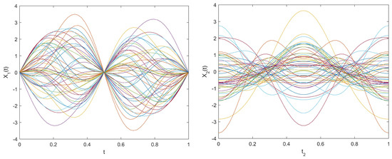
Figure 1. The predictors $X_1\left(t\right)$ and $X_2\left(t\right)$.

The scalar predictor $Z={(Z_1,Z_2,Z_3)}^T$ satisfies the following assumption

$$Z_1\sim N(0,1),Z_2\sim N(0,\frac{\sqrt{3}}{3}),Z_3\sim N(0,\frac{\sqrt{5}}{5}).$$

We assume that the regression coefficient functions of the functional predictors satisfy the following assumption

$${\beta }_1\left(t\right)=\sum _{k=1}^4{\chi }_{1k}{\rho }_{1k}\left(t\right),$$

$${\beta }_2\left(t\right)=\sum _{k=1}^3{\chi }_{2k}{\rho }_{2k}\left(t\right),$$

where ${\chi }_{1k}=\sqrt{\frac{1}{3k}},k=1,2,3,4$ and ${\chi }_{2k}=\sqrt{\frac{1}{3k}},k=1,2,3$. Moreover, we assume that the regression coefficients $\gamma ={({\gamma }_1,{\gamma }_2,{\gamma }_3)}^T$ of the scalar predictors satisfy ${\gamma }_1=\sqrt{2}/\phantom{\sqrt{2}2}2$, ${\gamma }_2=\sqrt{3}/\phantom{\sqrt{3}3}3$, ${\gamma }_3=1/2$.

Define

$$P(X,Z)=g\left(\sum _{j=1}^2{\int }_T{X}_j\left(t\right){\beta }_j\left(t\right)+Z^T\gamma \right).$$

And we select the link function as

$$g\left(x\right)=\frac{exp\left(x\right)}{1+exp\left(x\right)}.$$

We generate binary response

$$Y(X,Z)\sim Binomial\left(P\right(X,Z),1)$$

as pseudo random sequence.

We obtain a sample

$$(Y_i,X_{i1}\left(t\right),X_{i2}\left(t\right),Z_i),i=1,\dots ,n,$$

where n is the sample size. The number of functional principal components that explain 85% of cumulative variation contribution are $m_1=3,3,4$, $m_2=2,3,3$, respectively. We run 100 simulations.

Figure 2 shows the asymptotic behavior of the link function under different sample sizes. The black lines in Figure 2 shows the relationship between $\eta$ and $\mu$, where

$$\eta =\sum _{j=1}^2{\int }_T{X}_j\left(t\right){\beta }_j\left(t\right)dt+Z^T\gamma ,\mu =g\left(\eta \right)=\frac{exp\left(\eta \right)}{1+exp\left(\eta \right)}\in [0,1].$$

The additional colored lines shown in Figure 2 represent the estimated link function $\widehat{g}$ for different sample sizes. These lines are obtained through iterative processes, starting with an initial value of g set to $g\left(\eta \right)=\eta$. The iterative process continues until one of the following conditions is met: 100 iterations have been performed, or the error in the regression coefficients is less than 0.01. The purpose of these lines is to illustrate the relationship between $\widehat{\eta }$ and $\widehat{\mu }$, where

$$\widehat{\eta }=\sum _{j=1}^2{\int }_T{X}_j\left(t\right){\widehat{\beta }}_j\left(t\right)dt+Z^T\widehat{\gamma },\widehat{\mu }=\widehat{g}\left(\widehat{\eta }\right)\in [0,1].$$

Since in this case, both $\widehat{\eta }$ and $\eta$ are in $[-2,2]$, we denote the argument of g and $\widehat{g}$ by $\eta$, and the x-axis in Figure 2 is denoted by $\eta$ and is shown in the interval $[0,1]$. Table 2 presents the estimates of $\widehat{g}$ evaluated through RMISE under different sample sizes. The RMISE is defined as follows:

$$RMISE=\sqrt{\frac{1}{Q}{\int }_{-2}^2{(\widehat{g}\left(\eta \right)-g\left(\eta \right))}^{2}d\eta },$$

where $Q=100$ is the number of simulations here. In summary, Figure 2 and Table 2 demonstrate that as the sample size increases, the estimated link function $\widehat{g}$ becomes closer and closer to the true link function g.

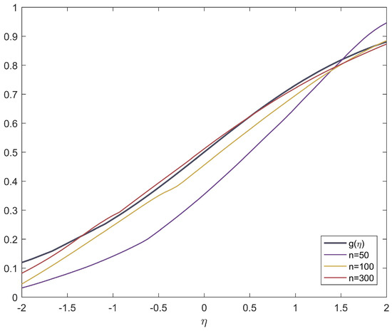
Figure 2. Asymptotic properties of the link function g. The black line in the graph represents the true link function $g=exp\left(\eta \right)/(1+exp(\eta \left)\right)$. The purple, yellow, and red lines in the graph represent the estimated link functions $\widehat{g}$ under sample sizes of $n=50$, $n=100$, and $n=300$, respectively.

Table 2. RMISE of g and $\widehat{g}$ for different sample size n.

n	RMISE
50	0.3540
100	0.2734
300	0.1449

In Table 3, it can be seen that both the SD and RMISE of the estimated regression coefficient functions ${\widehat{\beta }}_1\left(t\right)$ and ${\widehat{\beta }}_2\left(t\right)$ decrease as the sample size n increases.

Table 3. SD and RMISE of the estimated values of ${\widehat{\beta }}_1\left(t\right)$ and ${\widehat{\beta }}_2\left(t\right)$ for different sample sizes n.

	n	SD	RMISE
	50	0.2475	0.3405
${\widehat{\beta }}_1\left(t\right)$	100	0.1344	0.2517
	300	0.0552	0.1204
	50	0.2536	0.3232
${\widehat{\beta }}_2\left(t\right)$	100	0.1261	0.2863
	300	0.0239	0.1033

Figure 3 displays the estimated functional regression coefficients ${\widehat{\beta }}_1\left(t\right)$ and ${\widehat{\beta }}_2\left(t\right)$, as well as their 95% confidence intervals under different sample sizes. The red curve in the figure represents the theoretical values of ${\beta }_1\left(t\right)$ and ${\beta }_2\left(t\right)$, while the blue curve represents the estimated values ${\widehat{\beta }}_1\left(t\right)$ and ${\widehat{\beta }}_1\left(t\right)$. The gray shaded area represents the 95% confidence interval of the estimates. It can be seen that as the sample size increases, the estimated values become closer to the true values.

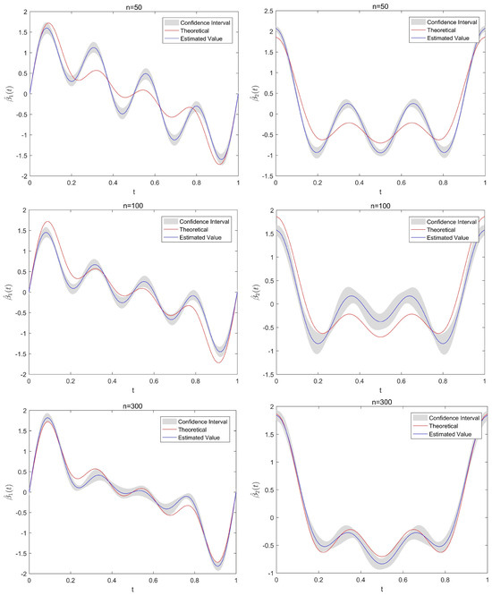
Figure 3. Estimated values of regression coefficient function ${\widehat{\beta }}_1\left(t\right)$, ${\widehat{\beta }}_2\left(t\right)$ (blue curves) and their 95% confidence intervals (grey area) for difference sample size, where the red curves are the theoretical regression coefficient functions ${\beta }_1\left(t\right)$, ${\beta }_2\left(t\right)$.

Table 4 presents the estimated scalar regression coefficient $\widehat{\gamma }$ and corresponding standard deviation under different sample sizes. It can be seen that as the sample size n increases, $\widehat{\gamma }={({\widehat{\gamma }}_1,{\widehat{\gamma }}_2,{\widehat{\gamma }}_3)}^T$ becomes closer to the true values $\gamma ={(\sqrt{2}/2,\sqrt{3}/3,1/2)}^T$. Moreover, as the sample size n increases, the SD becomes smaller, indicating that the estimated values have more certainty.

Table 4. Estimated values of scalar regression coefficients $\widehat{\gamma }$ and their SD in brackets for different sample sizes n.

n	${\widehat{\mathit{\gamma }}}_1$	${\widehat{\mathit{\gamma }}}_2$	${\widehat{\mathit{\gamma }}}_3$
50	0.7298 (0.191)	0.5928 (0.177)	0.5307 (0.232)
100	0.6892 (0.092)	0.5832 (0.071)	0.4894 (0.096)
300	0.7105 (0.019)	0.5732 (0.018)	0.4988 (0.016)

Table 5 presents the M1 and M2 values for different sample sizes, where $M1=\frac{1}{Q}{\sum }_{i=1}^{Q}MAE$, MAE= $\frac{1}{n}{\sum }_{i=1}^n|Y_i-{\widehat{Y}}_i|$, $M2=\frac{1}{Q}{\sum }_{i=1}^{Q}MSE$, MSE = $\frac{1}{n}{\sum }_{i=1}^n{(Y_i-{\widehat{Y}}_i)}^2$, and $Y_i$ and ${\widehat{Y}}_i$ represent the real and the predicted values of the response variable, respectively. We can find that as the sample size increases, the values of M1 and M2 become smaller, indicating that the predictive performance of the model improves.

Table 5. The M1 and M2 values for different sample sizes n.

n	M1	M2
50	0.3182	0.1579
100	0.3028	0.1498
300	0.2921	0.1406

6. Application

As is well known, research on average life expectancy is crucial for social development, health policies, and population management. Studies on average life expectancy can help governments, health departments, and social institutions develop relevant policies and plans to improve people’s quality of life and health conditions. By understanding people’s life expectancy, the efficiency of healthcare systems and the effectiveness of social welfare and public health policies can be evaluated, providing a basis for resource allocation and planning. Additionally, research on average life expectancy can also help people understand population structure and trends, providing references for social-economic development, pension systems, and labor market planning. Therefore, in the application of our proposed model, we investigate factors that influence average life expectancy, including air quality index (AQI), temperature, GDP, and number of beds in hospitals.

6.1. Data Description

We collected average daily temperature (Temp) data for 58 cities in China in 2020 from the National Meteorological Science Data Sharing Service Platform, and average daily Air Quality Index (AQI) data from the National Environmental Monitoring Station. We also collected GDP, number of beds in hospitals, and life expectancy data for each city from local statistical bulletins and government documents. Among them, there are two functional predictive variables, which are daily AQI and temperature from 1 January to 31 December 2020, for 366 days in 58 cities. There are also two scalar predictive variables, which are GDP and number of beds in hospitals for the 58 cities in 2020. The response variable is the life expectancy of residents in each city in 2020.

Figure 4 shows the daily AQI and temperature for 58 cities in 2020.

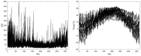
Figure 4. Daily AQI (left plot) and daily temperatures (right plot) for 58 cities in 2020; each curve represents one city.

6.2. Data Analysis

According to a report released by the National Health Commission, the average life expectancy of Chinese residents in 2020 was 77.9 years. Therefore, we divide the response variable as follows: when the life expectancy of a city is greater than 77.9 years, we represent it as 1; otherwise, when the life expectancy is less than 77.9 years, we represent it as 0. For the functional predictors, we first centralize the data. Second, we conduct FPCA and select the number of functional principal components that explain 75% of the variation. The number of components for AQI and temperature is $p_{AQI}=10$ and $p_{Temp}=3$, respectively. We use GCV to demonstrate the predictive accuracy of the estimators. In this application, $GCV=0.135$.

6.3. Results Analysis

By inputting the data into the generalized partially functional linear model, we obtain the regression coefficient function $\widehat{\beta }\left(t\right)$ for the functional predictors and the regression coefficients $\widehat{\gamma }$ for the scalar predictors. The results are shown in Table 6 and Figure 5, respectively.

Table 6. Regression coefficients $\widehat{\gamma }$ and their significance levels.

	Estimate	Std.Error	t Value	Pr (>$\left|\mathit{t}\right|$)
${\widehat{\gamma }}_{GDP}$	0.6776	0.339	1.9988	0.04639
${\widehat{\gamma }}_{Beds}$	0.7354	0.367	2.0038	0.04585

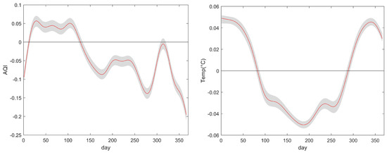
Figure 5. Estimated values of regression coefficient function $\widehat{\beta }\left(t\right)$ and their 95% confidence intervals.

Table 6 presents the estimated values of the regression coefficient $\widehat{\gamma }$ for scalar predictor variables. We can see that both GDP and number of beds in hospitals have a positive relationship with life expectancy, and are significant at the 5% level. This means that when a region has a higher GDP and more hospital beds, the life expectancy in that region is longer. In other words, the better the economic development and medical resources of a region, the longer the life expectancy.

In Figure 5, we see the estimated values of the regression coefficient function $\widehat{\beta }\left(t\right)$. For AQI, we can find a negative relationship between AQI and life expectancy in general. The higher the value of AQI, the more serious the air pollution is, and the lower the life expectancy corresponding to it. However, there is a more obvious positive relationship trend in February to April, which may be influenced by some other external factors. For temperature, we can find that the effect of temperature on life expectancy varies with the change of seasons. In spring, summer, and fall (March to October), the effect of temperature on life expectancy is negatively correlated, and in winter (November to February), it is positively correlated, which is consistent with the conclusion in Huang et al. [19].

To confirm the necessity of considering the unknown link function model, we choose models without a link function and with the logit link function (i.e., $g\left(\eta \right)=\frac{e^{\eta }}{1+e^{\eta }}$) and compare them with our proposed models with unknown link functions. In order to evaluate the prediction performance of the three models, we use MAE, MSE, and $R^2$. Additionally, we calculate the accuracy using the confusion matrix, where we define TP as the number of samples correctly classified as positive, TN as the number of samples correctly classified as negative, FP as the number of samples incorrectly classified as positive, and FN as the number of samples incorrectly classified as negative (missed detections). We obtain the model’s accuracy using the formula

$$Accuracy=\frac{TP+TN}{TP+TN+FP+FN}.$$

When the values of MAE and MSE are smaller, it indicates that the model has a smaller prediction error and better performance. When $R^2$ is closer to 1, it indicates that the model has a stronger ability to explain the response variable. The experimental results are shown in Table 7. It can be seen that the model we proposed has the best performance.

Table 7. Comparison between Unknown Link Function Model, Logit Link Function Model, and Model without a Link Function.

Link Function	MAE	MSE	${\mathit{R}}^2$	Accuracy
Unknown	0.2584	0.1399	0.8916	81.03%
Logit	0.2872	0.2511	0.6673	75.86%
Without	0.4777	0.3146	0.4118	74.14%

7. Conclusions

This article proposes a generalized partially functional linear model for scalar response and predictor variables that include both functional and scalar components, without specifying a link function. We use functional principal component analysis to reduce the dimensionality of functional data, estimate the regression coefficients using the maximum likelihood estimation method, estimate the link function using the method of local linear regression, iteratively obtain the final estimator, and establish the asymptotic normality of the estimator. The accuracy of the proposed model is validated through simulation studies.

The article applies the proposed model to the study of average life expectancy. Using daily AQI, temperature, GDP, and number of beds in hospitals for 58 cities in China in 2020, the study explores the impact of environmental, economic, and medical factors on life expectancy. The results indicate that GDP and number of beds in hospitals have a positive correlation with the life expectancy, while the AQI has an overall negative correlation. Temperature has a negative correlation with the average life expectancy in spring, summer, and autumn, and a positive correlation in winter. Overall, the study concludes that the average life expectancy is higher in areas with better environmental, economic, and medical development.

This model can be used in various fields, including economics, bio-medicine, engineering, etc. However, this model still has certain limitations. For example, the relationship between air quality and temperature needs to be further considered. There is a certain correlation between temperature and air quality. Generally, an increase in temperature can lead to the intensified volatilization and diffusion of pollutants in the air, thereby causing a decline in air quality. In the next phase of research, we will consider the interactions between functional predictors to make results more accurate. In addition, the algorithms and optimization methods of the model can be further improved to enhance computational efficiency. Combining this model with other machine learning methods can further improve predictive performance.

References

- Ramsay, J.O. When the data are functions. Psychometrika 1982, 47, 379–396. [Google Scholar] [CrossRef]
- Ramsay, J.O.; Silverman, B.W. Functional Data Analysis, 2nd ed.; Springer: New York, NY, USA, 2005. [Google Scholar]
- Horváth, L.; Kokoszka, P. Inference for Functional Data with Application; Springer: New York, NY, USA, 2012. [Google Scholar]
- Shin, H. Partial functional linear regression. J. Stat. Plan. Inference 2009, 139, 3405–3418. [Google Scholar] [CrossRef]
- Shin, H.; Lee, M.H. On prediction rate in partial functional linear regression. J. Multivar. Anal. 2012, 103, 93–106. [Google Scholar] [CrossRef][Green Version]
- James, G.M. Generalized linear models with functional predictors. J. R. Stat. Soc. Ser. B 2002, 64, 411–432. [Google Scholar] [CrossRef]
- Müller, H.G.; Stadtmüller, U. Generalized functional linear models. Ann. Stat. 2005, 33, 774–805. [Google Scholar] [CrossRef]
- Shang, Z.F.; Cheng, G. Nonparametric inference in generalized functional linear models. Ann. Stat. 2015, 43, 1742–1773. [Google Scholar] [CrossRef]
- Wong, R.K.W.; Li, Y.; Zhu, Z.Y. Partially Linear Functional Additive Models for Multivariate Functional Data. J. Am. Stat. Assoc. 2019, 114, 406–418. [Google Scholar] [CrossRef]
- Scallan, A.; Gilchrist, R.; Green, M. Fitting Parametric Link Functions in Generalized Linear Models. Comput. Stat. Data Anal. 1984, 2, 37–49. [Google Scholar] [CrossRef]
- Weisberg, S.; Welsh, A.H. Adapting for the missing link. Ann. Stat. 1994, 22, 1674–1700. [Google Scholar] [CrossRef]
- Chiou, J.M.; Müller, H.G. Quasi-likelihood regression with unknown link and variance functions. J. Am. Stat. Assoc. 1998, 93, 1376–1387. [Google Scholar] [CrossRef]
- Chiou, J.M.; Müller, H.G. Estimated estimating equations: Semiparametric inference for clustered and longitudinal data. J. R. Stat. Soc. Ser. B 2005, 67, 531–553. [Google Scholar] [CrossRef]
- Bai, Y.; Fung, W.K.; Zhu, Z.Y. Penalized quadratic inference functions for single-index models with longitudinal data. J. Multivar. Anal. 2009, 100, 152–161. [Google Scholar] [CrossRef]
- Pang, Z.; Xue, L. Estimation for the single-index models with random effects. Comput. Stat. Data Anal. 2012, 56, 1837–1853. [Google Scholar] [CrossRef]
- Yuan, M.; Diao, G. Sieve maximum likelihood estimation in generalized linear models with an unknown link function. Wiley Interdiscip. Rev. Comput. Stat. 2017, 10, e1425. [Google Scholar] [CrossRef]
- Kokoszka, P.; Reimherr, M. Introduction to Functional Data Analysis; CRC Press: Boca Raton, FL, USA, 2017. [Google Scholar] [CrossRef]
- Rao, A.R.; Reimherr, M. Nonlinear Functional Modeling Using Neural Networks. J. Comput. Graph. Stat. 2023, 32, 1248–1257. [Google Scholar] [CrossRef]
- Huang, C.; Barnett, A.G.; Wang, X.; Tong, S. The impact of temperature on years of life lost in Brisbane, Australia. Nat. Clim. Chang. 2012, 2, 265–270. [Google Scholar] [CrossRef]
- Yang, Y.; Qi, J.L.; Ruan, Z.L.; Yin, P.; Zhang, S.Y.; Liu, J.M.; Liu, Y.N.; Li, R.; Wang, L.J.; Lin, H.L. Changes in Life Expectancy of Respiratory Diseases from Attaining Daily PM2.5 Standard in China: A Nationwide Observational Study. Innovation 2020, 1, 100064. [Google Scholar] [CrossRef] [PubMed]
- Deryugina, T.; Molitor, D. The Causal Effects of Place on Health and Longevity. J. Econ. Perspect. 2021, 35, 147–170. [Google Scholar] [CrossRef]
- Mack, Y.P.; Silverman, B.W. Weak and strong uniform consistency of kernel regression estimates. Probab. Theory Relat. Fields 1982, 63, 405–415. [Google Scholar] [CrossRef]
- Masry, E.; Tjøstheim, D. Estimation and Identification of Nonlinear ARCH Time Series: Strong Convergence and Asymptotic Normality. Econom. Theory 1995, 11, 258–289. [Google Scholar] [CrossRef]
- Chiou, J.M.; Müller, H.G. Nonparametric quasi-likelihood. Ann. Stat. 1999, 27, 36–64. [Google Scholar] [CrossRef]
- Xiao, W.W.; Wang, Y.X.; Liu, H.Y. Generalized partially functional linear model. Sci. Rep. 2021, 11, 23428. [Google Scholar] [CrossRef] [PubMed]
Disclaimer/Publisher’s Note: The statements, opinions and data contained in all publications are solely those of the individual author(s) and contributor(s) and not of MDPI and/or the editor(s). MDPI and/or the editor(s) disclaim responsibility for any injury to people or property resulting from any ideas, methods, instructions or products referred to in the content. |
© 2023 by the authors. Licensee MDPI, Basel, Switzerland. This article is an open access article distributed under the terms and conditions of the Creative Commons Attribution (CC BY) license (https://creativecommons.org/licenses/by/4.0/).