Abstract
Most time series from real-world processes are stained with noise. Therefore, much attention should be paid to data noise removal techniques. In this study, we use the family of biorthogonal wavelet, high-pass, and low-pass filters, to investigate the power of the wavelet method in removing noise from time series data. Using the wavelet discrete transformation, the variability of precipitation and sea surface temperature is analyzed for a southern region of the Caspian Sea. At each stage of decomposition, the previous wave is decomposed into two waves. In this research, the SST and precipitation data are decomposed into several levels based on discrete wavelet transformation. In each level of decomposition, the previous wave is decomposed into two waves. This can be done many times and at each stage, reducing the amount of data. This method is reversible, and the original wave can be reconstructed using the decomposed values. In the study of discrete wavelet transforms, it was observed that the analysis based on wavelets leads to more accurate results. The reconstruction error in the proposed method is shown to be very small.
Keywords:
Fourier transform; wavelet analysis; climate data time series; dynamic analysis; southern Caspian Sea; variability MSC:
65T60; 65T50
1. Introduction
Numerous socioeconomic processes are impacted by the hydroclimate variations within a region. Droughts and wet spells are part of the hydroclimate variability. It is crucial to research the causes of historical hydroclimate variability given the potential societal effects of hydroclimate variability. The examination of large data sets and modeling are the two main methods used to understand hydroclimate variability. Time series of climate data can be affected by various disturbances and errors caused by different systems, climate change, and asynchronous issues [1,2,3]. Therefore, it is important to extract the actual time series signals from the noisy data (e.g., natural disasters, pandemics, and financial data [4,5,6,7]).
The wavelet method is very effective in dealing with noisy data due to its multi-resolution nature. The wavelet method is a prominent method that can pave the way in the analysis of different types of data. As a result, wavelet analysis is widely utilized in domains such as astronomy, electronics, and seismology, as well as economics and finance, and it is now being employed for temperature analysis [8].
Studies show that observational climatic time series data have measurement errors that are referred to as climatic data series noise. This makes the analysis and prediction of data less accurate. The wavelet method is used to de-noise the time series of standard climatic data, which is an unstable signal because it can express the signal in both time and frequency ranges (or scales), as well as handle local analysis of the signal.
A common method for noise reduction is the Fourier transform, which is used in signal analysis and processing. Using the Fourier transform, a signal is decomposed into sinusoidal factors, i.e., the frequencies that make up the signal. But this conversion has its limitations. Mathematically, the wave transform provides more information than the raw data [9]. By wave transformation in the frequency domain, we can see better information from the wave. Using the frequency spectrum, one can observe the frequency content of the wave, which represents the rate of change. If the variable is constant over time in the frequency spectrum, its frequency is zero. If the changes are fast, the wave frequencies are high, and if the changes are small, the frequencies are low.
The Fourier transform, with all its capabilities, has its drawbacks. In this method, the base wave is a sine wave that extends uniformly from ∞- to ∞+. While the frequency content of each sine wave is a point, it sometimes causes instability in non-harmonic waves. The Fourier transform essentially identifies the wave’s frequency content and does not reveal when each frequency appears. To solve this problem, a Fourier piecewise transform is used. Although the Fourier piecewise transforms convert the time of occurrence of each frequency, an important parameter in this method is the proper choice of the width and height of the window function. Proper selection of the window function will have a significant effect on the final result. The width of the window, in unstable waves, may destroy the reliability of the selected part. A steady wave is a wave whose constituent frequencies occur the whole time of the wave occurrence, and an unstable wave is a wave that has different frequencies at different moments [10,11].
To solve the problems of the Fourier transform, the wavelet transform method is used. In this method, instead of using harmonic functions, other functions known as mother and scale functions are used [10]. To distinguish various wave frequencies, the mother functions are employed in continuous transforms, while the mother and scale functions are utilized in wavelet discrete transforms. Some mother functions have explicit mathematical relationships, whereas others do not [12].
In this study, the signal from climatic data is first passed through two low and high pass filters, after which two waves, known as the approximate wave and the partial wave, are formed, with and indicated in each stage. The problem is that at each level, using filters, the main wave is split into two waves with the same number of points, thereby doubling the number of wave points.
The down-sampling method is used to address this issue [13]. The number of points on each wave is roughly half that of the main wave in the sampling reduction strategy since one of two subsequent points is maintained and the other is deleted. After this stage, the number of wave points can still be decreased.
Because the highest wave energy in the approximation wave and its shape is similar to those of the main wave, the filtering method is performed on this portion of the wave, and the wave is split into two waves, and , each with about half the number of points as the wave.
Although this can be done in a hypothetical order (N is the number of wave points), dynamic analysis requires a wave that is very similar to the original wave and has a minimal number of points. According to research, implementing this approach in three stages reduces the dynamic analysis error by less than 10% and the analysis time by around 90% [14,15].
Wavelet discrete transformation acts as a filter bank. A filter bank is a set of low and high pass filters that, by combining them simultaneously with each other, can decompose a wave into its constituent frequencies or reconstruct the wave from its constituent frequencies. In this research, the Mallat method is used [16].
In the analysis of multi-resolution problems, we can refer to the work of Vasilios et al., which used wavelets to analyze the temperature relationship in 22 patients with and without fever at different frequency scales [17]. They realized that the temperature rises and falls over different frequency scales due to the intensity and decrease in fever. Zahavi and Rosenstein modeled temperature dynamics using wavelets in the Ornstein–Olenbeck process with constant oscillation [18]. Qixuan used the multicellular wavelet method for the non-standing measurement of temperature series in the province of Alberta [19]. In this research, the study of severe temperature fluctuations observed in winter due to unpredictable winds can be considered one of the important reasons for insurance. Manimaran et al. used the wavelet multi-resolution method to analyze time series at critical temperatures [20]. Schleswig et al. used wavelet transformation to analyze the average annual air temperature with time-varying time series data [21]. Wavelet transform-based noise removal to reduce the temperature error of temperature sensors was also performed by Wang et al. [22]. More examples of the application of the multi-resolution wavelet method can be found in Xiaomei et al. [23], Emmanuel et al. [24], Longo et al. [25], Zhang et al. [26], Gallegati et al. [27], and Tamilselvi and Thangaraj [28], while the application of multi-resolution can be seen in Tan & Qiu [29], and other studies.
Nalley et al. carried out wavelet analysis using a discrete wavelet transform to detect surface temperatures in Ontario, Quebec, and Canada as a whole [30]. Fredriksen investigated the linear conversion of wavelet variance logarithms to estimate the Hearst parameter in temperature time series [31]. Kwon et al. used wavelet coefficients as inputs of a self-reversing model to provide time-frequency, temperature, and precipitation characteristics [32]. Finally, a third type of application that deals with the elimination of raw data noise can also be found in several articles. Nason’s work examined the issue of threshold parameter selection for estimating wavelet functions [33]. Camps and Tarongi considered the wavelet threshold techniques to eliminate noise to reduce microwave hazards [34]. Schimmack et al. used wavelet packets to eliminate bus temperature sensor noise [35]. Anctil and Coulibaly used wavelets to describe the climatic diversity of southern Quebec using the first component in a local climate cycle [36].
Abdolkarim et al. demonstrate the utility of wavelets in temperature data noise reduction [37]. A key reference on how wavelets can be employed in the study of water surface temperature time series and heat flow components of a hydroelectric reservoir was provided in [38]. A recent paper by Xiaohong et al. combined a wavelet transform model and support a cutting machine developed to predict temperature time series, which works especially well with rainfall and temperature time series [39]. By converting wavelets to other times and scales, we may decompose time series and identify their attributes in different frequency bands, such as time [40]. In multi-resolution time series analysis, this strategy is typically employed [41].
In this research, we focus on two important parameters, sea surface temperature (SST) and precipitation, as the most effective factors affecting the climate of the Caspian Sea investigated in the recent literature. Then, we present the results of the use of the wavelet transform to demonstrate new insights gained from the use of wavelet transforms.
2. Materials and Methods
2.1. Materials
We made use of ERA5′s monthly mean SST and precipitation data. The examined dataset, ERA5, has a high geographic resolution of 0.25° latitude/longitude and is the most recent reanalysis data available from the European Centre for Medium-Range Weather Forecasts (ECMWF) [42]. The data used in the research area—the South Caspian Sea—cover a 42-year time span beginning in 1979 and ending in 2021.
The Caspian Sea is the largest landlocked water body in the world and has three main geomorphological and oceanographic districts: the southern, middle, and northern regions (Figure 1). The area of the southern Caspian Sea, our study area, is about 148,640 square kilometers, which includes approximately 39.3% of the total area and 65.5% of the total volume of the sea. The average depth of the South Caspian Sea is about 345 m and its volume is less than two-thirds of the Caspian Sea as a whole. The physical environment of the Caspian Sea, as well as atmospheric cycles passing over the heights of its coastlines, influence its climate. Due to its location in low latitudes, the Caspian Sea receives a considerable amount of sunshine.
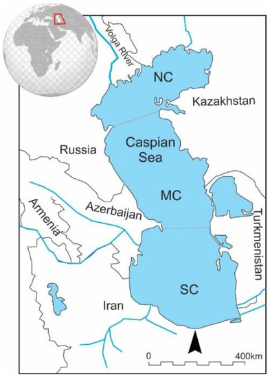
Figure 1.
General map of the Caspian Sea and its location (the inset). SC: south Caspian Sea, MC: Middle Caspian Sea, and NC: North Caspian Sea domains.
On the Caspian Sea, the annual total solar energy intake is around 3700 kWh. This has an impact on the climate of the Caspian Sea, particularly in the southern and western regions of the Alborz and Caucasus mountains, as well as the steppes and deserts in the eastern part. The Caspian Sea region’s climate is influenced by the cold Arctic and humid air masses of the Atlantic Ocean, the dry and cold continental region of Kazakhstan, and the tropical tropics traveling through the Mediterranean Sea and Iran.
In most circumstances, the sea is warmer on average than the coast, except in the second part of spring and summer, when the opposite is true. In the western and central regions of the Caspian Sea, February is when it becomes coldest [3].
The temperature of the Caspian Sea is not constant across all areas due to its large area. Water temperatures vary annually in the northern, central, and southern parts. Changes in water temperature occur not only at the surface but also different depths. There are two main reasons for the temperature difference in the Caspian Sea: one is the latitude and the other is the different depths of the sea. The water temperature changes with latitudes. The temperature difference decreases in spring in the northern and southern parts of the Caspian Sea. This decrease is more evident in early summer, and, at this time, the sea surface water temperature is almost the same in all three parts of the Sea. While in the northern Caspian Sea average sea surface temperature ranges between freezing temperature in winter to >25 °C in summer, the SST of the southern Caspian Sea oscillates between >7 °C in winter and >25 °C during summer.
Our study area was limited to the southern region of the Caspian Sea. The meteorological information used in this study was taken from ECMWF-ERA5, which was continuously updated in real time. These datasets offer monthly data from 1979 through 2020 together with long-term time series [42].
2.2. Methods
The time series of the SST and precipitation in the South Caspian Sea for the average of two seasons, summer and winter, was chosen. For summer, we take the average of the June, July, and August data and for the winter we choose the average of the December, January, and February data.
Herein, we detail the wavelet discrete transform procedure for time series data decomposition. Approximate and partial wave coefficients of climatic data waves are obtained using Equations (1) and (2):
where k is an integer, and stand for low-pass filter and high-pass filter, respectively, is the vector of the climate data time series, n is the number of climate data, and j denotes the number of the decomposition stage. Equations (3)–(6) are applied to derive values for and from one stage to the next:
The above relationships demonstrate the method’s resemblance to the filter hypothesis and wavelet discrete transform, which correspond to the filter bank decomposition and composition, respectively. Equation (7) can also be used to rebuild the main wave:
where corresponds with but they must be equal to each other. The difference between the initial wave and the reconstructed wave is very small (Table 1). Filters , , , , which are used for wave decomposition and reconstruction, are obtained using Equation (8) [16]:

Table 1.
Maximum error in reconstruction for SST and precipitation time series.
Also, QMF is assumed as Equation (9):
Additionally, in this research, for the scaling function , we assume Equations (10) and (11) [13]:
3. Wavelet
Wavelets are mathematical functions that separate the data into their constituent frequency components and define each component by the power of separation or resolution corresponding to the scale of that component. The main advantage of the wavelet transform compared to the Fourier transform is its high power of analysis in situations where the data has discontinuities and rapid jumps. In the theory of wavelets, if the study window is large, the general characteristics of the time series can be seen, and if the study window is small, the details will be more informative. In this transformation, the data is analyzed by using the basic wavelet and by scaling and time shifting this wavelet. The larger the scale used, the more the fundamental wavelet is stretched, and the analysis will be done on the low-frequency components of the information. Conversely, the smaller the scale used, the more the fundamental wavelet is compressed, and the analysis is performed on the high-frequency components. Wavelet transform is the decomposition of a function based on wavelet functions. Wavelets are shifted and scaled samples of a function (mother wavelet) with finite length and strongly damped oscillation.
3.1. Wavelet Discrete Transformation
A signal can be divided into numerous dimensions using the wavelet transform, and each dimension can be treated independently. The idea of a band-pass filter is similar including how Fourier transforms process independent signals into different frequency sine waves [14]. Wavelet analysis can reveal signal characteristics in both the temporal and frequency domains.
The following is the definition of the wavelet transform [43,44,45]. Given a function , where is the space composed of a square integral function in real space, make a displacement τ before making an inner product with the signal that is to be analyzed in different dimensions. The wavelet transform of is:
The discrete wavelet transform is significant and necessary when dealing with real-time signals. In many other applications, we make each dimension binary discrete. The wavelet equation will be as follows if we assume ,:
Suppose that , then the discrete wavelet transform equation becomes:
For decomposing the signal to obtain the binary wavelet coefficient in various dimensions, we must first decompose the sampling signal into N dimensions using the suitable wavelet basis function. In this study, we deconstruct and reconstruct signals using biorthogonal wavelet bases, such as “coif”, “Symlet”, and others.
An efficient method for decomposing a wave into high and low frequencies is the use of filters [16]. The Mallat algorithm is a well-known classical scheme in wave processing and is known as two-channel encryption. In this method, one wave enters, and two waves, which contain the main wave coefficients, exit.
The low-frequency content is the most vital component of the wave, whereas the high frequency represents the wave’s specific features.
For example, if a signal’s high-frequency components are not included, although the new signal is different, it will still behave in the same way as the original signal, and its properties can be analyzed. However, if a signal is sufficiently removed from the low frequencies, the new signal is no longer recognizable and has new components from which the characteristics of the original signal cannot be accessed.
We frequently discuss the approximation and partial waves when discussing wavelet discretization. The low-frequency portion of the wave is represented by the approximation wave and the high-frequency portion by the partial wave. The main S wave is put through two complimentary high and low pass filters in this procedure, resulting in the creation of two additional waves. The wave that represents the low frequencies is called the approximate wave () and the wave that represents the high frequencies is called the partial wave ().
By carrying out this process on a wave signal, the number of wave points is doubled. For example, if the original wave has N points, each of the output signals will have N points and the total number of points will increase to 2N points.
One approach for lowering the number of points is to use the sampling reduction method. In this method, the points are removed one by one. By doing this operation, the number of wave points is halved, and the sum of the number of points of the two waves is equal to that of the original wave. The waves produced at this stage ( and ) each have approximately N/2 points. To better understand this process, the separating a wavelet transform of a wave is shown in Figure 2. In this example, the principal wave resembles a sine function to which high-frequency noise is added.
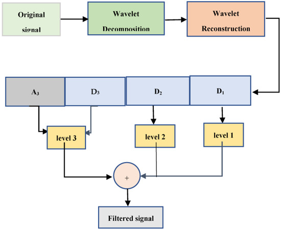
Figure 2.
Signal decomposition and reconstruction process.
It is clear from Figure 2 that the partial coefficients of small and noise include high frequencies. Although at this stage the approximate coefficients () have a small amount of noise, this is much less than that of the main wave and can be reduced by repeating this process.
3.2. Multistage Decomposition
The decomposition process described above can be repeated and the approximate wave obtained in each step can be decomposed into two waves. This is called wavelet step decomposition (Figure 3). Theoretically, this decomposition can be done in a number order. However, in dynamic analysis, we require a wave that is highly similar to the original wave and has a small number of points.
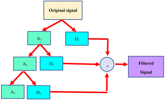
Figure 3.
Wavelet multistage decomposition of the decomposed signal’s information.
The ability of the wavelet transform to function as a digital filter under the right conditions is a crucial attribute that was uncovered throughout the experiments. Figure 2 illustrates the signal breakdown and reconstruction methods.
3.3. Choosing the Proposed Filter Using the Wavelet Function
In this study, the wavelet transform serves as a digital filter. In order to locate the wavelet function with the fewest coefficients and least amount of signal distortion after filtering, it was decided to conduct a study. The energy of each wavelet function served as our initial criterion for selection.
The function to be applied would be the one with the lowest coefficients and the highest average amount of stored energy. In the experiment, a collection of epileptiform occurrences was applied using well-known wavelet functions. In common with Symlets, Coiflets, and other wavelet families, we adopted biorthogonal wavelet function families.
4. Wave Reconstruction
The signal wave can be rebuilt using this method without losing the original wave information. Inverse discrete wavelet transformation is the name of the reconstruction method. For wave decomposition and reconstruction, the sampling reduction method is applied, and we also apply the method of increasing sampling (upsampling) (↑). In this process, the number of data is increased by adding zeros in the data [44].
Cumulative reflective filters consist of high-pass and low-pass decomposition filters (L and H) that are dependent on reconstruction filters. The total number of decomposition and reconstruction filters resembles a mirrored image.
The main wave can be reconstructed using approximate and partial wave coefficients (Figure 3). Due to the low effect of partial wave coefficients (D) on wave reconstruction, only approximate coefficients (A) can be used and zero is used in place of D coefficients. Although this removes a lot of the main wave’s high frequencies, the difference between the generated wave and the main wave is not significant and can be ignored [45].
The time series signal is decomposed and reassembled into three levels in this investigation, providing an approximation level as well as six levels of detail, , , and . The degree of decomposition of the decomposed signal is used to categorize each frequency component of the original signal.
When a signal is recreated from a specified level of approximation or detail, only the frequencies that specifically cover this level will be used to imitate it. In other words, certain bands from the original signal have been divided into secondary reconstructed signals (, , , and ). The reconstructed signals are combined to create the original signal. Conversely, comparing them produces a signal with no particular frequencies. These factors led to the development of a digital filter that could be used in localization and object recognition processes for preparing time series data signals using the wavelet transform.
In the initial testing with epileptiform episodes, the signals were broken down and reassembled into three levels, producing the levels of detail and the level of approximation . Each level of specificity was examined independently.
The features of the generated signal were observed to be its morphology, amplitude, and repeatability at the detail level, which produces the largest number of reconstructed signals that are morphologically similar to the original signal. In the level of detail , , and , we noticed a recurrent pattern that corresponded to the frequency band defined for the epileptiform occurrences.
The low frequencies of the original signal were preserved via the approximation according to experiments. This was eventually validated by studies. The epileptiform event frequencies are included in the signal generated as a result of this technique. Therefore, the signal is devoid of the noise frequencies and contains all the frequencies needed for accurate epileptiform event reconstruction (Figure 3). To collect a signal devoid of interference, such as baseline and low-frequency oscillations, as well as high-frequency interference, this filter is intended to add levels of detail.
5. Results
This section presents the results of the analysis of the wavelet functions that work best with the suggested filter. The experiments consisted of calculating correlations using a set of epileptiform data time series.
5.1. Decomposition of Climate Data Time Series
Table 1 shows the amount of wave reconstruction error and the data time series decomposition of the various seasons in various stages. We show the wavelet decomposition of data time series over three levels. The signal begins with a leap, which is followed by a smooth wave of rising frequency. The smooth part’s singularity and frequency can be seen in the discrete wavelet transform (DWT).
5.1.1. Decomposition of SST Data
The time series of the SST in the South Caspian Sea for the averages DJF and JJA are shown in Figure 4. Figure 5, Figure 6 and Figure 7 represent the decomposition of the data time series from the first to third stages. As can be seen, the A coefficients curve is extremely similar to the wave of the previous stage and contains the main wave information.
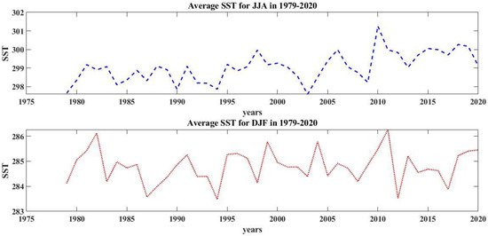
Figure 4.
Average SST for JJA and DJF months in the period 1979–2020.
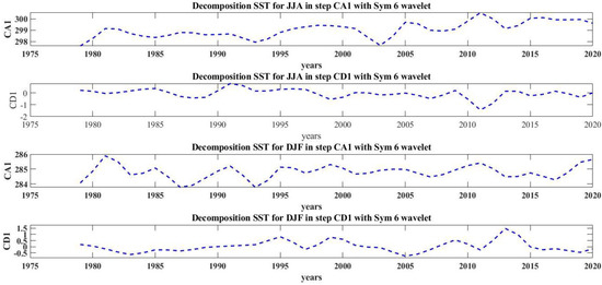
Figure 5.
Level−1 decomposition for SST in the JJA and DJF months.
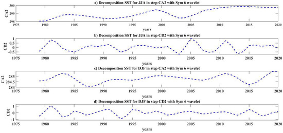
Figure 6.
Level−2 decomposition for SST in the JJA and DJF months.
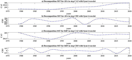
Figure 7.
Level−3 decomposition for SST in the JJA and DJF months.
5.1.2. Decomposition of Precipitation Data
The time series of the precipitation in the South Caspian Sea for the averages DJF and JJA are shown in Figure 8. Figure 9, Figure 10 and Figure 11 show the decomposition of the first to third stages of the data time series. As can be seen, the A coefficient curve includes the majority of the wave’s information and is extremely similar to the wave from the step before.
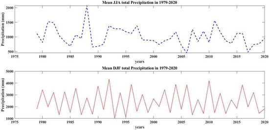
Figure 8.
Average JJA and DJF total precipitation (mm) in the period 1979−2020.
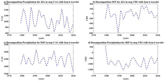
Figure 9.
Level−1 decomposition for precipitation in the JJA and DJF months.
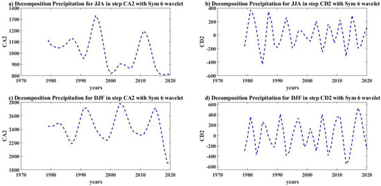
Figure 10.
Level−2 decomposition for precipitation in the JJA and DJF months.
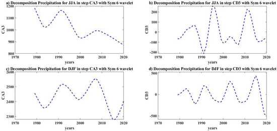
Figure 11.
Level−3 decomposition for precipitation in the JJA and DJF months.
Using the results obtained from the analysis in the previous data, it is observed that at each stage the A curve is very similar to the A curve in the previous stage, and only its partial fractures are removed. In dynamic analysis, the moment-by-moment analysis time is sometimes reduced by reducing the number of data points. This sometimes removes important points from the data time series. Using each of the As, the structure can be dynamically analyzed and then reconstructed dynamically with a reverse process. If great care is taken, the signal can be analyzed against D and the final solution can be obtained by combining the A and D responses. Research in this field has shown that with the removal of D, the signal response will remain largely the same.
The influence of the combination of multiple frequency factors on the temperature fluctuation structure may be seen in the calculated trend values of the approximation component compounds. On an annual basis, two frequency combinations dominate as oscillation patterns.
These findings suggest that temperature oscillates under the influence of both high and low frequencies at the same time and in a complicated manner. The effect of short-term events on temperature fluctuation behavior, such as the amount of solar radiation, the angle of radiation, and so on, are linked to high frequencies. Low and high frequencies suggest the presence of relatively rare events.
This scenario is mirrored in the findings of a seasonal and yearly time series analysis, with the major frequency in seasonal data being the combined component of high and low frequencies, but it is more frequent in annual data. Given the long-term time base of annual data (in comparison to seasonal and short-term data), a combination of low and long-term frequencies seems suitable.
The low-frequency behavior of the JJA and DJF seasons is more similar, which is understandable in the study of temperature data in different seasons. This could indicate that in these seasons, the behavior of temperature limitations (which is influenced by low and long-term frequencies) is more similar. The existence of a high-frequency component in all these seasons is significant.
5.2. Wavelet Function Selection for Use with the Suggested Filter
In this paper, the wavelet transform serves as a digital filter. In order to determine the wavelet function that would work best with the filter—one with few coefficients and little signal distortion after filtering—a study was conducted.
The energy of each wavelet function served as our initial criteria for selection. The function to be used would be the one with the lowest number of coefficients and the highest average amount of collected energy. The experiment involved using existing wavelet functions to apply a set of epileptiform occurrences. We employed the same biorthogonal wavelet function families as Symlets, Coiflets, and others.
Each of the wavelet functions chosen for this investigation was subjected to all epileptiform episodes. Each deconstructed epileptiform event’s energy was calculated, then accumulated and used to calculate the energy average of each wavelet function used. Seven functions with the highest cumulative average energy were chosen for testing with the suggested filter. Table 2 shows the results.

Table 2.
Visualization of the seven wavelet functions with the highest energy values and their respective number of coefficients for the epileptiform events used.
A period of the data time series signal containing an epileptiform event, low-frequency oscillations, high frequency, and noise was utilized to test the generated function. The filtered signals are shown in Figure 12 and Figure 13 after this signal was subjected to the Coiflet functions from Table 2.
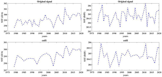
Figure 12.
Wavelet filtering for SST time series in JJA and DJF with Coiflet functions.
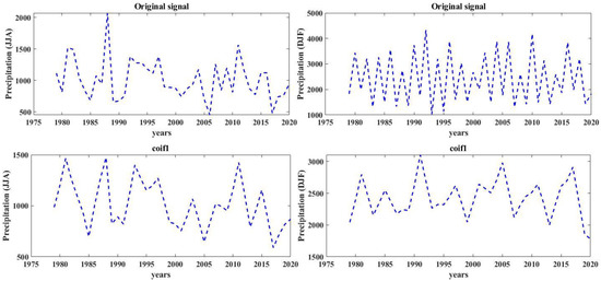
Figure 13.
Wavelet filtering for precipitation time series in JJA and DJF with Coiflet functions.
5.3. Wavelet Analysis
Figure 14 shows the time series of yearly SST data in mean warm and cold seasonal data alongside the wavelet power spectrum related to SST data from 1979 to 2020. For both time series graphs (Figure 14a,b), SST trends are ascending, while the warm season slope is steeper than that of the cold season (which is linked to global warming). The results confirm the pick signals of the power spectrum analysis by revealing that events between data periods are completely different, exception for four to eight periods between 2007 to 2016. For the warm season, pick signals are observed for between three- and six-year periods from 2000 to the end of the data period. Conversely, energetic annual and semi-annual scale signals only are observed in the years 2010 to 2012 (Figure 14c). For the cold season mean, energetic signals are lower than the warm season mean, i.e., pick signals are observed in the warm season but the number of energetic signals occurrences is greater in the cold season mean. They occurred in four- to eight-year periods before the year 2000 and fewer than six-year periods after 2000. Generally, it can be observed that annual and semi-annual signals were observable from 1999 to the end of the measurement period.
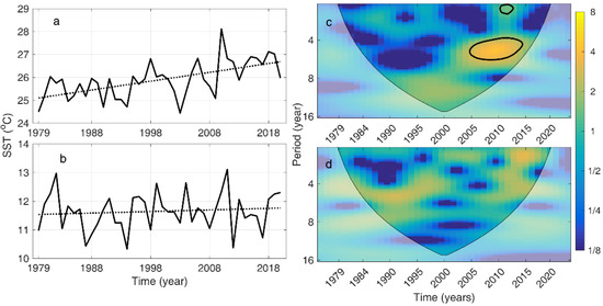
Figure 14.
Yearly time series of SST and related trends in (a) JJA and (c) DJF and Morlet wavelet power spectrum of the SST in (b) JJA and (d) DJF.
Wavelet coherency results between synchronous yearly SST and precipitation from 1979 to the end of 2020 are shown in Figure 15. The effects of precipitation are observed in different time scales and years for both warm and cold mean SST. Regions with low coherence coincide with low wavelet power in the SST and are therefore expected. For about 11 years (from 1984 to 1995), high coherence is observed in both warm and cold seasons for annual and semi-annual scales. Another high coherence is observed for less than two years scale in the warm season (Figure 15a) suggesting that precipitation passively mirrors SST. For the warm season, the first significant sector is located at periodicities of 1–36 months, between 1984 and 1999. The second one is located for an up to two years period between 2008 and 2016. Arrows indicate an anti-phase relationship in the latter. Another significant coherency between SST and precipitation is located in four– to six-year periods from 2010 to 2017 led by . Unlike the warm season, precipitation improves SST in the time scale of six to eight years, from 1984 to 2007 during the cold season (Figure 15b). In the time scale of four to six years, it was mostly in phase from 1984 to 1998, the SST lead precipitation by from 1998 to 2003, and, finally, from 2003 to 2010 precipitation improves SST again in a time scale of about six years. Generally, precipitation had a different effect on SST in the two different seasons.
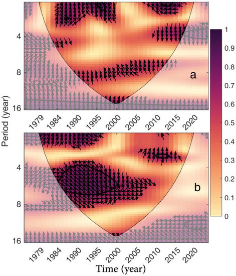
Figure 15.
Wavelet coherence and the phase difference between the yearly SST data and precipitation, (a) in JJA, and (b) DJF.
6. Conclusions
Using the wavelet discrete transform method, high and low frequencies of data time series can be easily obtained. This can be done many times. Obviously, the further the decomposition goes, the lower the frequencies of the data time series. This method is reversible and the original wave can be reconstructed from the approximate and partial waves. The reconstruction error in this method is very low. It is obvious that having separate frequencies of data time series (low and high frequencies), makes it easier to analyze the system against high and low frequencies and, if necessary, the signal can be analyzed for each of these frequencies.
The results revealed that the original signal’s low-frequency oscillations and high-frequency noise were reduced, leaving just the epileptiform episodes to be highlighted. However, due to the properties of each wavelet function, the event takes on different shapes depending on which one is employed.
Various tests were run to see which wavelet function best kept the form of the epileptiform episodes after processing, while also attenuating high- and low-frequency noise. In order to assess these differences between the original signals and the filtered signals, the corresponding error with the change in the signal’s morphology was evaluated. The method was revealed to be very powerful for analyzing time series originated from real-world processes.
Author Contributions
Data collection, M.M.-A.; study conception, J.A., analysis and interpretation of results, M.M.-A. and O.N., editing, A.M.L. and A.N.B. All authors have read and agreed to the published version of the manuscript.
Funding
This research received no external funding.
Data Availability Statement
Not applicable.
Acknowledgments
We are grateful that we were allowed to use the ERA5 due to the license to use Copernicus Products according to regulation (EU) No. 377/2014 of the European Parliament and to the reviewers who provided suggestions on how to improve the manuscript.
Conflicts of Interest
The authors declare no conflict of interest.
References
- Arpe, K.; Molavi-Arabshahi, M.; Leroy, S.A.G. Wind variability over the Caspian Sea, its impact on Caspian seawater level and link with ENSO. Int. J. Climatol. 2020, 40, 6039–6054. [Google Scholar] [CrossRef]
- Lau, W.K.M.; Kim, K. The 2010 Pakistan Flood and Russian Heat Wave: Teleconnection of Hydrometeorological Extremes. J. Hydrometeorol. 2021, 13, 392–403. [Google Scholar] [CrossRef]
- Molavi-Arabshahi, M.; Arpe, K.; Leroy, S.A.G. Precipitation and temperature of the southwest Caspian Sea region during the last 55 years: Their trends and teleconnections with large-scale atmospheric phenomena. Int. J. Climatol. 2015, 35, 2156–2172. [Google Scholar] [CrossRef]
- Yang, C.; Sha, D.; Liu, Q.; Li, Y.; Lan, H.; Guan, W.W.; Hu, T.; Li, Z.; Zhang, Z.; Thompson, J.H.; et al. Taking the pulse of COVID-19: A spatiotemporal perspective. Int. J. Digit. Earth 2022, 13, 1186–1211. [Google Scholar] [CrossRef]
- Pagnottoni, P.; Spelta, A.; Flori, A.; Pammolli, F. Climate change and financial stability: Natural disaster impacts on global stock markets. Phys. A Stat. Mech. Its Appl. 2022, 599, 127514. [Google Scholar] [CrossRef]
- Yu, M.; Yang, C.; Li, Y. Big Data in Natural Disaster Management: A Review. Geosciences 2018, 8, 165. [Google Scholar] [CrossRef]
- Pagnottoni, P.; Spelta, A.; Pecora, N.; Flori, A.; Pammolli, F. Financial earthquakes: SARS-CoV-2 news shock propagation in stock and sovereign bond markets. Phys. A: Stat. Mech. Its Appl. 2021, 582, 126240. [Google Scholar] [CrossRef]
- Yun, H.; Jun, L. Teleconnection between climate oscillations and riverine nutrient dynamics in Southeast China based on wavelet analysis. Environ. Sci. Pollut. Res. 2021, 28, 41807–41820. [Google Scholar] [CrossRef]
- Morlet, J. Sampling Theory and Wave Propagation. In Issues in Acoustic Signal—Image Processing and Recognition; NATO ASI Series (Series F: Computer and System Sciences); Chen, C.H., Ed.; Springer: Berlin/Heidelberg, Germany, 1983; Volume 1. [Google Scholar] [CrossRef]
- Sunjay, S. Sequence Stratigraphy by Wavelet Analysis of Well Logging Data. In Proceedings of the International Conference on Recent Develop-ments in Stratigraphy, Pune University, Pune, India, 12–18 December, 2013. [Google Scholar]
- Torrence, C.; Compo, G.P. A Practical Guide to Wavelet Analysis. Bull. Am. Meteorol. Soc. 1998, 79, 61–78, Retrieved 28 October 2022. [Google Scholar] [CrossRef]
- Jiangtao, X.; Pingpinfg, L. Application of Wavelet Analysis in the Prediction of Telemetry Data. Int. J. Adv. Netw. Monit. Control. 2019, 4, 28–34. [Google Scholar] [CrossRef]
- Strang, G.; Nguyen, T. Wavelets and Filter Banks; Wellesley-Cambridge Press: New York, NY, USA, 1996. [Google Scholar]
- Pandey, B.K.; Tiwari, H.; Khare, D. Trend analysis using discrete wavelet transform (DWT) for long-term precipitation (1851–2006) over India. Hydrol. Sci. J. 2017, 62, 2187–2208. [Google Scholar] [CrossRef]
- Timoshevskaya, O.; Londikov, V.; Andreev, D.; Samsonenkov, V.; Klets, T. Digital data Processing Based on wavelet transforms. In Proceedings of the Environment Technology Resources Proceedings of the International Scientific and Practical Conference, 17–18 June 2021; Volume 2, pp. 174–180. [Google Scholar] [CrossRef]
- Mallat, S. A theory for multiresolution signal decomposition: The wavelet representation. IEEE Tran. Pat. Anal. Mach. Intel. 1989, 11, 674–693. [Google Scholar] [CrossRef]
- Papaioannou, V.E.; Chouvarda, I.G.; Maglaveras, N.K.; Pneumatikos, I.A. Temperature variability analysis using wavelets and multiscale entropy in patients with systemic inflammatory response syndrome, sepsis, and septic shock. Crit. Care 2012, 16, R51. [Google Scholar] [CrossRef] [PubMed]
- Zahavi, G.; Rosenstein, Y. Weather Derivative Pricing with Nonlinear Weather Forecasting. 21 May 2012. ACRN Journal of Finance and Risk Perspectives. ISSN 2305-7394. Available online: https://ssrn.com/abstract=2204179 (accessed on 22 May 2011). [CrossRef]
- Qixuan, Z. Dynamic Moment Analysis of Non-Stationary Temperature Data in Alberta. Master’s Thesis, Faculty of Management, University of Lethbridge, Lethbridge, AB, Canada, 2008. [Google Scholar]
- Manimaran, P.; Panigrahi Prasanta, K.; Parikh Jitendra, C. Wavelet analysis and scaling properties of time series. Phys. Rev. E J. 2005, 72, 046120–046125. [Google Scholar] [CrossRef]
- Sleziak, P.; Hlavčová, K.; Szolgay, J. Advantages of a Time Series Analysis Using Wavelet Transform as Compared with a Fourier Analysis. Slovak J. Civ. Eng. 2015, 23, 30–36. [Google Scholar] [CrossRef]
- Wang, Z.; Lv, G.; Chang, J.; Zhang, S.; Luo, S.; Jia, C.; Jiang, S.; Sun, B.; Liu, Y.; Liu, X. An Improved Denoising Method in RDTS Based on Wavelet Transform Modulus Maxima. IEEE Sens. J. 2015, 15, 1061–1067. [Google Scholar] [CrossRef]
- Xiaomei, S.; Xu, Y.; Yan, C. Wavelet Analysis of Rainfall Variation in the Yellow River Basin. Acta Scicentiarum Nat. Univ. Pekinesis 2006, 42, 503–509. [Google Scholar]
- Emmanuel, C.N.; Gerardo, R.J.; Anatoly, M. Wavelet analysis for spectral inversion of seismic reflection data. J. Appl. Geophys. 2020, 177, 104034. [Google Scholar] [CrossRef]
- Longo, C.; Burr, T.; Myers, K. Change Detection Using Wavelets in Solution Monitoring Data for Nuclear Safeguards. Axioms 2013, 2, 271–285. [Google Scholar] [CrossRef]
- Zeng, K.; Chen, D.; Ouyang, G.; Wang, V.; Liu, X.; Li, X. An EEMD-ICA Approach to Enhancing Artifact Rejection for Noisy Multivariate Neural Data. IEEE Trans. Neural Syst. Rehabil. Eng. 2016, 24, 630–638. [Google Scholar] [CrossRef] [PubMed]
- Gallegati, M.; Ramsey, J.B.; Semmler, W. Time Scale Analysis of Interest Rate Spreads and Output Using Wavelets. Axioms 2013, 2, 182–207. [Google Scholar] [CrossRef]
- Tamilselvi, P.R.; Thangaraj, P. Noise suppression and improved edge texture analysis in kidney ultrasound images. In Proceedings of the International Conference on Innovative Computing Technologies (ICICT), Karur, India, 12–13 February 2010; pp. 1–6. [Google Scholar] [CrossRef]
- Tan, M.; Qiu, A. Spectral Laplace-Beltrami Wavelets with Applications in Medical Images. IEEE Trans. Med. Imaging 2012, 34, 1005–1017. [Google Scholar] [CrossRef] [PubMed]
- Nalley, D.; Adamowski, J.; Khalil, B.; Ozga-Zielinski, B. Trend detection in surface air temperature in Ontario and Quebec, Canada during 1967–2006 using the discrete wavelet transform. Atmos. Res. 2013, 132–133, 375–398. [Google Scholar] [CrossRef]
- Fredriksen, H.B. Long-Range Memory in Earth Surface Temperatures: Spatial Scale Dependence and Land-Sea Differences. Master’s Thesis, Faculty of Science and Technology, Department of Physics and Technology, University of Tromsø, Tromsø, Norway, 2013. [Google Scholar]
- Kwon, H.H.; Lall, U.; Khalil, A.F. Stochastic simulation model for nonstationary time series using an autoregressive wavelet decomposition: Applications to rainfall and temperature. Water Resour. Res. 2007, 43, W05407. [Google Scholar] [CrossRef]
- Nason, G.P. Choice of the Threshold Parameter in Wavelet Function Estimation. In Wavelets and Statistics. Lecture Notes in Statistics; Antoniadis, A., Oppenheim, G., Eds.; Springer: New York, NY, USA, 1995; Volume 103. [Google Scholar] [CrossRef]
- Camps, A.; Tarongi, J.M. RFI Mitigation in Microwave Radiometry Using Wavelet. Algorithm 2009, Algorithm 2, Algorithm 1248, Algorithm 1249, Algorithm 1250, Algorithm 1251, Algorithm 1252, Algorithm 1253, Algorithm 1254, Algorithm 1255, Algorithm 1256, Algorithm 1257, Algorithm 1258, Algorithm 1259, Algorithm 1260, Algorithm 1261 and Algorithm 1262 2009, 2, 1248–1262. [Google Scholar] [CrossRef]
- Schimmack, M.; Nguyen, S.; Mercorelli, P. Implemented Wavelet Packet Tree based Denoising Algorithm in Bus Signals of a Wearable Sensorarray. J. Phys. Conf. Ser. 2015, 659, 1–9. [Google Scholar] [CrossRef]
- Anctil, F.; Coulibaly, P. Wavelet Analysis of the Interannual Variability in Southern Quebec Streamflow. J. Clim. 2004, 17, 163–173. [Google Scholar] [CrossRef]
- Abdul Karim, S.A.B.; Ismail, M.T.; Hasan, M.K.; Sulaiman, J. Denoising the temperature data using wavelet transform. Appl. Math. Sci. 2013, 7, 5821–5830. [Google Scholar] [CrossRef][Green Version]
- de Alcântara, E.H.; Stech, J.L.; Lorenzzetti, J.A.; de Moraes, E.M.L. Time series analysis of water surface temperature and heat flux components in the Itumbiara Reservoir (GO), Brazil. Acta Limnol. Bras. 2011, 23, 245–259. [Google Scholar] [CrossRef][Green Version]
- Xiaohong, L.; Shujuan, Y.; Li, L. Prediction of Temperature Time Series Based on Wavelet Transform and Support Vector Machine. J. Comput. 2012, 7, 8. [Google Scholar] [CrossRef][Green Version]
- Tangborn, A. Wavelet approximation of error covariance propagation in data assimilation. Tellus A Dyn. Meteorol. Oceanogr. 2004, 56, 16–28. [Google Scholar] [CrossRef]
- Jianmin, F.; Xu, L.; Zhi, Z. Analysis on Multi-Scale Features of Precipitation in East and Middle Part of Northwest China and West Mongloia. Sci. Meteorol. Sin. 2005, 25, 474–482. [Google Scholar]
- Hersbach, H.; Bell, B.; Berrisford, P.; Biavati, G.; Hor_anyi, A.; Muñoz, S.J.; Nicolas, J.; Peubey, C.; Radu, R.; Rozum, I.; et al. ERA5 monthly averaged data on single levels from 1979 to present. Copernicus Climate Change Service (C3S) Climate Data Store (CDS) 2020, [Data Set]. Available online: https://doi.org/10.24381/cds.f17050d7 (accessed on 28 October 2022).
- Colombo, F.; Magazu, S.; Caccamo, M.T. Wavelet Analysis as a Tool for Characterizing Trends in Climatic Data. January 2018. Available online: https://hdl.handle.net/11570/3126996 (accessed on 28 October 2022).
- Akujuobi, C.M. Wavelets and Wavelet Transform Systems and Their Applications; Springer: Cham, Switzerland, 2022. [Google Scholar]
- Bhatnagar, N. Introduction to Wavelet Transforms. Chapman and Hall/CRC: New York, NY, USA, 2020. [Google Scholar]
Disclaimer/Publisher’s Note: The statements, opinions and data contained in all publications are solely those of the individual author(s) and contributor(s) and not of MDPI and/or the editor(s). MDPI and/or the editor(s) disclaim responsibility for any injury to people or property resulting from any ideas, methods, instructions or products referred to in the content. |
© 2022 by the authors. Licensee MDPI, Basel, Switzerland. This article is an open access article distributed under the terms and conditions of the Creative Commons Attribution (CC BY) license (https://creativecommons.org/licenses/by/4.0/).