Application of the Methodology of Multi-Valued Logic Trees with Weighting Factors in the Optimization of a Proportional Valve

Abstract

Hydraulic valves are used to determine the set values of hydraulic quantities (flow rate, pressure, or pressure difference) in a hydraulic system or its part. This is achieved through the appropriate throttling of the stream flowing through the valve, which is automatically set by the operator (e.g., opening the throttle valve). The procedures for determining its static and dynamic properties were described using the example of modeling a two-stage proportional relief valve. Subsequently, the importance of the design and operational parameters was determined using multi-valued logic trees. Modeling began with the determination of equations describing the flow and movement of moving parts in a valve. Based on the equations, a numerical model was then created, e.g., in the Matlab/Simulink environment (R2020b). The static characteristics were obtained as the result of a model analysis of slow changes in the flow rate through the valve. Various coefficients of logical products have not been taken into account in the separable and common minimization processes of multi-valued logic equation systems in any available literature. The results of the model tests can be used to optimize several types of hydraulic valve constructions.

1. Introduction

In recent years, intensive development in the field of hydraulic valves has been observed. This development is mainly related to the integration of electronics designed to control the valves. Modern hydraulic valves—especially those controlled via the proportional technique—are often equipped with various types of sensors, e.g., an inductive spool-position sensor inside the body of a proportional valve. The integration of classic hydraulics with electronics and sensors creates new, previously unattainable possibilities for using hydraulic proportional valves [1]. The course of the control signal of proportional valves is shown in the form of a block diagram in Figure 1.

An analog electrical signal with a voltage value typically not greater than 10 V is fed to an electronic amplifier. From the electronic amplifier, the electric control signal is fed through wires with a current that usually does not exceed 1.5 A per coil of a proportional electromagnet. Depending on the type of proportional electromagnet, a force or displacement of the proportional electromagnet armature is generated. If the valve uses a proportional solenoid with an adjustable stroke, a displacement of the electromagnet armature is generated proportionally to the value of the control current. This affects the proportional valve’s control element (e.g., a spool-bushing pair or seat plug), causing its displacement (x). If the valve uses a proportional solenoid with a regulated force, the F force is generated proportionally to the value of the control current on the armature of the proportional solenoid. This force is transmitted to the valve control, which is usually a poppet in the proportional pressure valve. With a change in the displacement of the valve actuator or the force acting on it, the Q flow rate or the p pressure functionally vary depending on if a proportional valve is controlling the flow rate or pressure. These parameters control the operation of the hydraulic receiver where the current determines the n or v speed of the hydraulic receiver and the pressure determines the external M or F load.

There are no significant differences in terms of the mechanical design between conventionally controlled valves and proportionally controlled valves. The main difference relies on the fact that, in proportional valves, instead of a spring, hand wheel, lever, or conventional solenoid, there are one or more proportional solenoids. There are two types of proportional electromagnets: force-adjustable and stroke-adjustable. Their use depends on the type and function of the proportional valve and is determined by its characteristics. The benefits of using proportional valves include combining several functions in one valve, a smooth control of flow and pressure parameters, the ability to program the valve and the receiver controlled by it, and the reduction of dynamic surpluses [2]. Proportional valves also have some disadvantages in comparison to conventional ones, including a higher price, stricter requirements regarding purity of the working liquid, and sensitivity to operating conditions (moisture, salinity of the environment, and external mechanical vibrations). Technically speaking, proportional valves were initially a bridge between conventionally (mechanically or electrically) controlled valves and servo valves. Presently, the latest proportional control valves have dynamic parameters equal to those of servo valves and sometimes even surpass them [3]. For example, it can be stated that the limit frequency of a two-stage servo valve is 240–270 Hz depending on the manufacturer, and the limit frequency of the latest-generation proportional valve with VCD (Voice Coil Drive) technology is 350 Hz. Several years ago, this frequency was 6–10 Hz for a single-stage proportional valve [4]. In many industries, particularly mechanical engineering, proportional relief valves with one—or more often, two—stages are widespread. An example of the use of proportional valves is their use in the hydraulic system for lifting and lowering loads with significant masses [5] such as agricultural machinery [6], CNC machine tools, hydraulic presses, wheel loaders, and ships.

Related Work

The research to determine the importance of hydraulic valves’ design and/or operational parameters is still ongoing. For example, study [7] optimized the relief valve by minimizing partial multi-valued logic functions. Multi-valued logical equations which constituted design guidelines for the entire series of types of such valves were used. The analysis of the stability of hydraulic elements based on the systems of multi-valued logical equations and the method of multi-valued logical trees, taking into account weighting factors, allows for the consideration of the conditions of global stability. The most favorable result is the relationship specification, which binds the design and operational parameters limitations. In addition, the conditions that limit the parameters of the valve and the system are brought to a simple analytical and graphical relationship. Overall, it is limited to a relief valve system operated directly, general stability conditions, and a computerized time-course solution with different variable coefficients.

The modeling of hydraulic systems usually uses ordinary differential equations. From these equations a system of equations is created, initial conditions are assumed, and, after parameterization of the equations, the equations are solved to obtain time courses of the relevant parameters of the hydraulic system, e.g., pressure as a function of time or the velocity of the receiver as a function of time. These are models with focused parameters. One hydraulic system sometimes exhibits wave phenomena that lead to hydraulic resonance. This is referred to as a hydraulic long line. In such cases, partial differential equations are used for modeling and the method of characteristics (MOC) is used to solve them. This paper considers a system in which no wave phenomena occur and uses ordinary differential equations to describe the valve state. Decision-support systems are also applied to hydraulic and pneumatic systems [8,9,10,11,12,13,14,15,16]. The paper [8] mainly presents related methods, from classical clustering and classification topics to database methods (e.g., association), and from database methods (e.g., association rules, data cubes) to newer and more advanced topics (e.g., SVD/PCA, wavelets, support vector machines). The work of [9,10,11,12] focused on concepts for integrating decision-support systems of poorly structured data with a data warehouse based on relational or multidimensional structures. In [13], a framework was developed to evaluate different rainwater-discharge options for urban areas in arid regions. The modeling of rainfall runoff was carried out using the Hydrological-Engineering-Centre and Hydrological-Modelling-System (HEC-HMS). Hydraulic modeling was carried out using SewerGEM to evaluate the effectiveness of the various alternatives for a given design flood [14,15]. The authors of [14,15] presented further applications of multi-criteria decision support methods. In particular, in the work [15] of the Geospatial Information System (GIS), a multi-criteria decision-making system (MCDM) was applied to logic. The decision-making Trial and Evaluation Laboratory (DEMATEL) approach was used to create a network of relationships between criteria. The author of [17] described a model-driven decision-support system (software tool) implementing a model-based online leak-detection and localization methodology that is useful for a large class of water distribution networks.

The present work presents the use of multi-valued logical trees with multivalent weighting factors in the analysis of a two-stage proportional relief valve and a nozzle-aperture preliminary stage [18,19,20]. A significant amount of literature exists on the applications of decision trees in decision-making systems. However, there are only a small number of publications on their application in design methodology. Cognitive decision theories seek sufficient and effective solutions for so-called real-world problems and well-defined problems. There are a number of decision-support methods that are familiar to the authors and, in particular, have already been used by the authors to solve a number of problems in decision-support areas, e.g., in the use of special types of parametric dependency graphs [21,22]; inductive decision trees [23,24]; and in particular multi-valued logic trees [25]. Specifically, the recent paper has shown how methods based on multi-valued logic trees can be very beneficial when other methods are ineffective. However, multi-valued logic tree methods have plenty of advantages in design methodology and are still being developed. The advantage of the method of multi-valued logical trees is that the measurement data can be recorded by means of appropriate formal notations and it is even possible to combine complex quantitative and qualitative features with different degrees of detail according to the rules of the multi-valued morphological array. The canonical alternative normal form (KAPN) of a bivariate or multi-valued logical function describes all variants, i.e., true (realizable) solutions of a given problem obtained according to the rules of the morphological table, as the full array of combinations of values of logical variables describes all theoretical variants. As a result of minimization (after applying the Quine–McCluskey algorithm), one obtains from the realizable solutions the true sub-solutions as a shortened alternative normal form of the SAPN of the logical function. In this way, the real sub-solutions of the problem are appropriately grouped and therefore the computational time required to obtain the most important real sub-solutions is reduced.

2. The Tested Object

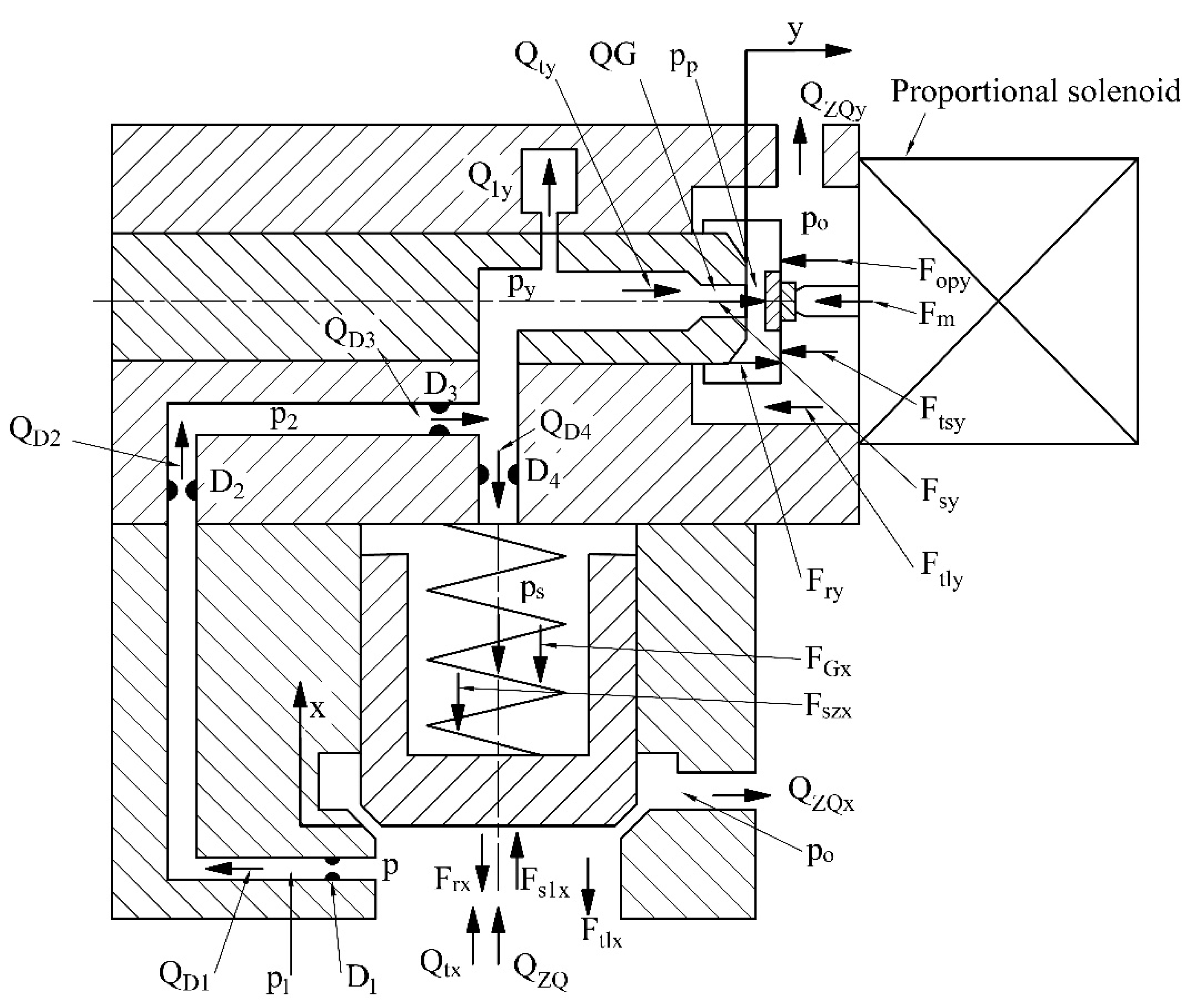
The tested object is a two-stage proportional relief valve with a preliminary nozzle-aperture stage (Figure 2) [23]. Figure 2 demonstrates a two-stage proportional relief valve. The main stage is pressure controlled, while the pilot is controlled by a proportional solenoid. Changing the pressure in the chamber above the main-stage spool is possible by throttling the fluid flowing out of the pilot. This throttling is altered by changing the position of the diaphragm driven by the proportional solenoid.

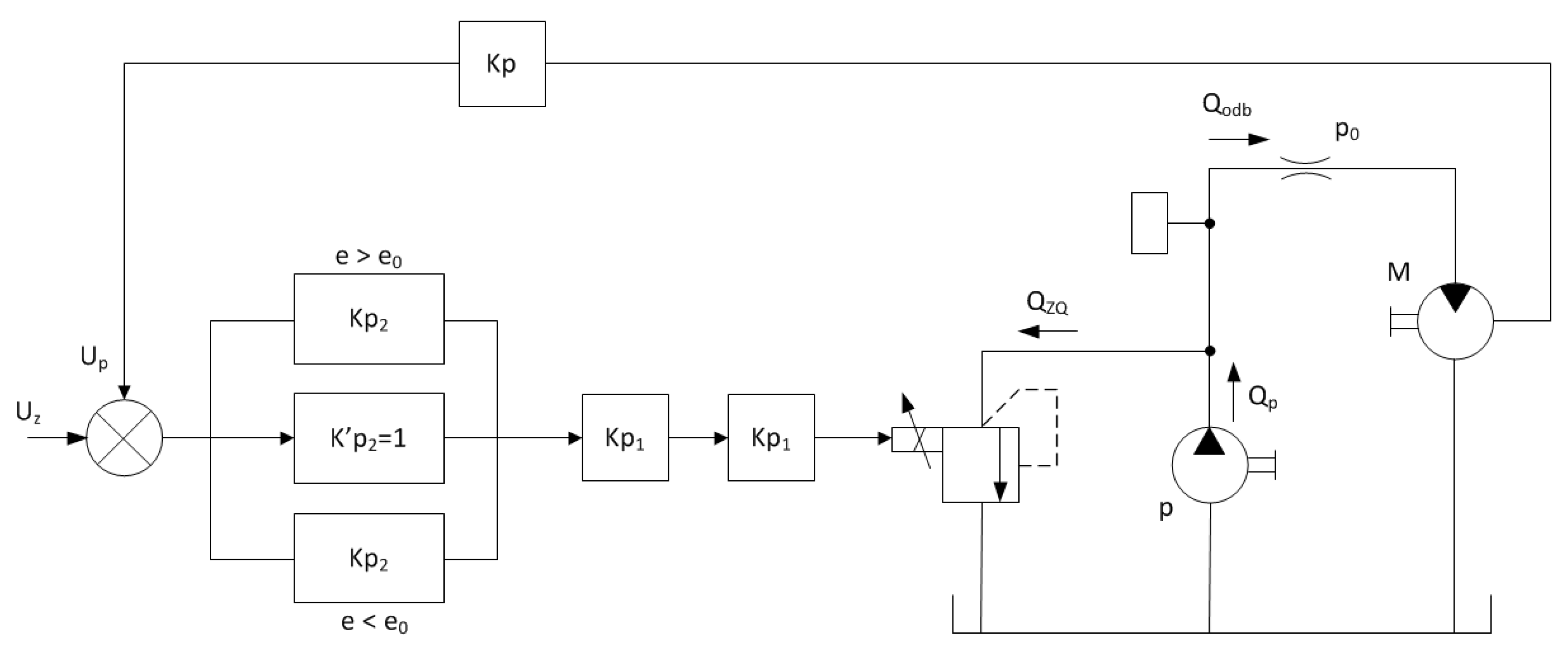
Figure 3 shows the drive system with a proportional valve and a receiver.

The receiver in the analyzed system is a throttle valve whose performance characteristics are described as follows:

$$\left\{\begin{array}{l}p\le 1 MPa:Q_{odb}=1.2446666\cdot {10}^{-10}p,\\ 1 MPa\le p\le 6 MPa:Q_{odb}=0.3533333\cdot {10}^{-10}p+0.8913333\cdot {10}^{-4},\\ p\le 6 MPa:Q_{odb}=0.2425893\cdot {10}^{-10}p+14.55\cdot {10}^{-5}.\end{array}\right.$$

(1)

where Q_odb is the hydraulic actuator flow rate.

In order to describe the flow through a proportional valve it is necessary to consider the value of the loss factor as a function of the displacement of the moving element. The actual course is similar to the solution of a second-order differential equation with a variable throttling factor. This relationship is described in the following form [26]:

$$\begin{array}{l}{k}_{vx}=0.82\cdot [1{-}^{}\exp (-b\cdot {10}^3\cdot \frac{x}{2})\cos ({10}^3\sqrt{-\mathrm{\Delta }})],\\ \mathrm{\Delta }<0\end{array}$$

(2)

where:

$$\begin{array}{l}b=5+\frac{5\cdot {10}^7}{p};\\ \mathrm{\Delta }=b^2-100{\pi }^2,\\ \mathrm{\Delta }>0\end{array}$$

(3)

and

$$k_{vx}=0.82[1{-}^{}\exp (-b-\sqrt{-\mathrm{\Delta }}){10}^3\frac{x}{2}].$$

(4)

The following course was used in the control stage ($\mathrm{\Delta }y<0$):

$$\begin{gathered} k_{vy}=0.75\left[1-\exp \left(-b_y·{10}^3·\frac{y}{2}\right)\cos \left({10}^{3}y\sqrt{-\mathrm{\Delta }y}\right)\right] \\ \mathrm{\Delta }y>0 \end{gathered}$$

(5)

where:

$$\begin{array}{l}{b}_y=40+\frac{1.5\cdot {10}^8}{p_y+{10}^5},\\ \mathrm{\Delta }y=b_y^2-100{\pi }^2.\end{array}$$

(6)

The force generated by the electromagnetic transducer used in the valve is described as follows:

$$\begin{array}{l}{F}_m=73.19631(i-0.045),\\ di=\frac{1}{T_m}(\frac{U}{18}-i)dt,\end{array}$$

(7)

where $T_m=15 \mathrm{ms}$ when i increases $\left(\frac{U}{18}-i>0\right)$ and $T_m=7.5 \mathrm{ms}$ when i decreases $\left(\frac{U}{18}-i<0\right)$.

Mathematical Model of the Tested Valve

The mathematical model of the valve under consideration was built on the basis of ordinary differential equations of the second order. The first equation of the system of equations is the flow rate balance equation, which takes into account the compressibility of the working fluid (its capacitance).

The flow balance of the drive system can be written as [23]:

$$Q_p=Q_{zQ}+Q_{1x}+Q_{odb}.$$

(8)

The flow balance through the main valve stage is described as:

$$Q_{zQ}=Q_{zQx}+Q_{D1}+Q_{tx}.$$

(9)

The flow through the nozzle is described as:

$$Q_{D1}=Q_{D2}=Q_{D3},$$

(10)

$$Q_{DG}=Q_{zQY}+Q_{tY}.$$

(11)

The flow balance through the control stage is described as:

$$Q_{D3}=Q_{1Y}+Q_{zQY}+Q_{tY}.$$

(12)

In addition, the flow rate is distinguished in the main stage as:

$$Q_{1x}=\frac{V_x}{B}\cdot \frac{dp}{dt}=\frac{4.33735\cdot {10}^{-3}}{1.4\cdot {10}^9}\frac{dp}{dt}=3.098107\cdot {10}^{-12}\frac{dp}{dt},$$

(13)

and at the control stage as:

$$Q_{1y}=\frac{V_y}{B}\cdot \frac{dp}{dt}=\frac{1.2\cdot {10}^{-6}}{1.4\cdot {10}^9}\frac{dp}{dt}=0.857\cdot {10}^{-15}\frac{dpy}{dt},$$

(14)

The flow rate through the valve is represented as:

$$\begin{array}{l}{Q}_z=\sqrt{\frac{2}{\rho }\cdot }k(k_{v}x)\sqrt{p-p_0},\\ \mathrm{with}\\ p_0\ll p,\end{array}$$

(15)

• through the main stage:

$$Q_{zQx}=\sqrt{\frac{2}{892}}\cdot \pi \cdot 22\cdot {10}^{-3}\cdot \sin 30°(k_{vx}\cdot x)\sqrt{p},$$

(16)

$$Q_{zQx}=1.6355097\cdot {10}^{-3}(k_{vx}\cdot x)\sqrt{p},$$

(17)

• through the control stage:

$$Q_{zQy}=\sqrt{\frac{2}{892}}\cdot \pi \cdot 1.8\cdot {10}^{-3}(k_{vy}\cdot y)\sqrt{p},$$

(18)

$$Q_{zQy}=0.2676292\cdot {10}^{-3}(k_{vy}\cdot y)\sqrt{p}.$$

(19)

Ultimately, the flow rates are represented as:

• through the nozzle D₁:

$$Q_{D1}=a_1(p-p_1)=0.2370513\cdot {10}^{-10}(p-p_1).$$

(20)

• through the nozzle D₃:

$$Q_{D3}=a_3(p_2-p_y)=0.2370486\cdot {10}^{-10}(p_2-p_y).$$

(21)

An additional equation described is the equilibrium equation of the forces acting on the valve control element (according to d’Alembert’s principle) on the main stage and the secondary stage. This equation takes into account the forces of inertia, spring stiffness, frictional force, and the hydrodynamic reaction force associated with the change in momentum of the fluid stream.

Forces in the valve:

Dynamic loads:

$$F_d=m\frac{d^{2}x}{d{t}^2},$$

(22)

In the main stage:

$$F_{dx}=\left[0.675+\frac{1}{3}(0.008+0.00439)\right]\frac{d^{2}x}{d{t}^2}=0.70631\frac{d^{2}x}{d{t}^2},$$

(23)

where the following values indicate:

• 0.0675—the mass of the main stage slider;
• 0.008—spring mass;
• 0.00439—the mass of the associated liquid.

In the control stage:

$$F_{dy}=0.03\frac{d^{2}y}{d{t}^2}.$$

(24)

Sticky friction:

$$F_{t1}=\frac{A_{st}\cdot \mu }{L_0}\cdot \frac{dx}{dt},$$

(25)

• forces in the main stage:

$$F_{t1x}=\frac{\pi \cdot 22\cdot {10}^{-3}\cdot 10.5\cdot {10}^{-3}\cdot 0.06265}{5\cdot {10}^{-6}}=9.0885102\frac{dx}{dt},$$

(26)

• forces in the control stage:

$$F_{t1y}=\frac{32\cdot {10}^{-6}\cdot 0.06265}{12\cdot {10}^{-6}}\frac{dy}{dt}=0.1670666\frac{dy}{dt}.$$

(27)

Forces of the hydrodynamic reaction are described as follows:

• of the main stage:

$$F_{rx}=2k_x\cos \theta (k_{vx}x)p=2\cdot \pi \cdot 22\cdot {10}^{-5}\cdot \sin 30°\cdot 1\cdot \cos 35°(k_{vx}x)p,$$

(28)

$$F_{rx}=56.59033\cdot {10}^{-6}\cdot (k_{vx}x)p,$$

(29)

• of the nozzle-aperture pair:

$$F_{ry}=\frac{16A_y{(k_{vy}y)}^2}{d_{DG}^2}{P_p}^{\prime }$$

(30)

$$F_{ry}=\frac{16\cdot \pi /4(1.65\cdot {10}^{-3})}{{(1.5\cdot {10}^{-3})}^2}{\left(k_{vy}y\right)}^2=15.1976{\left(k_{vy}y\right)}^2{P}_p.$$

(31)

The dynamic equations of the proportional valve forces are described at any point in the transient state after the introduction of the step function:

of the main stage:

$$F_{dx}=-F_{t1x}-F_{rx}-F_{szx}-F_{Gx}+F_{s1x}-F_{s2x}.$$

(32)

of the control stage:

$$F_{dy}=-F_{t1y}+F_{ry}+F_{sy}-F_{tsy}-F_{opy}-F_m.$$

(33)

The feedback loop equation is written as follows:

when U_z − U_p − e₀ < 0,

$$\frac{du}{dt}=K_M⌈K_{p1}(U_z-U_p)+K_{p2}\left(U_z-U_p-e_0\right)⌉,$$

(34)

when U_z − U_p + e₀ < 0,

$$\frac{du}{dt}=K_M⌈K_{p1}(U_z-U_p)+K_{p2}\left(U_z-U_p+e_0\right)⌉,$$

(35)

if none of these conditions are met:

$$\begin{gathered} -e_0<U_z-U_p<e_0, \\ \mathrm{to} \\ \frac{du}{dt}=K_M{K}_{p1}\left(U_z-U_p\right). \end{gathered}$$

(36)

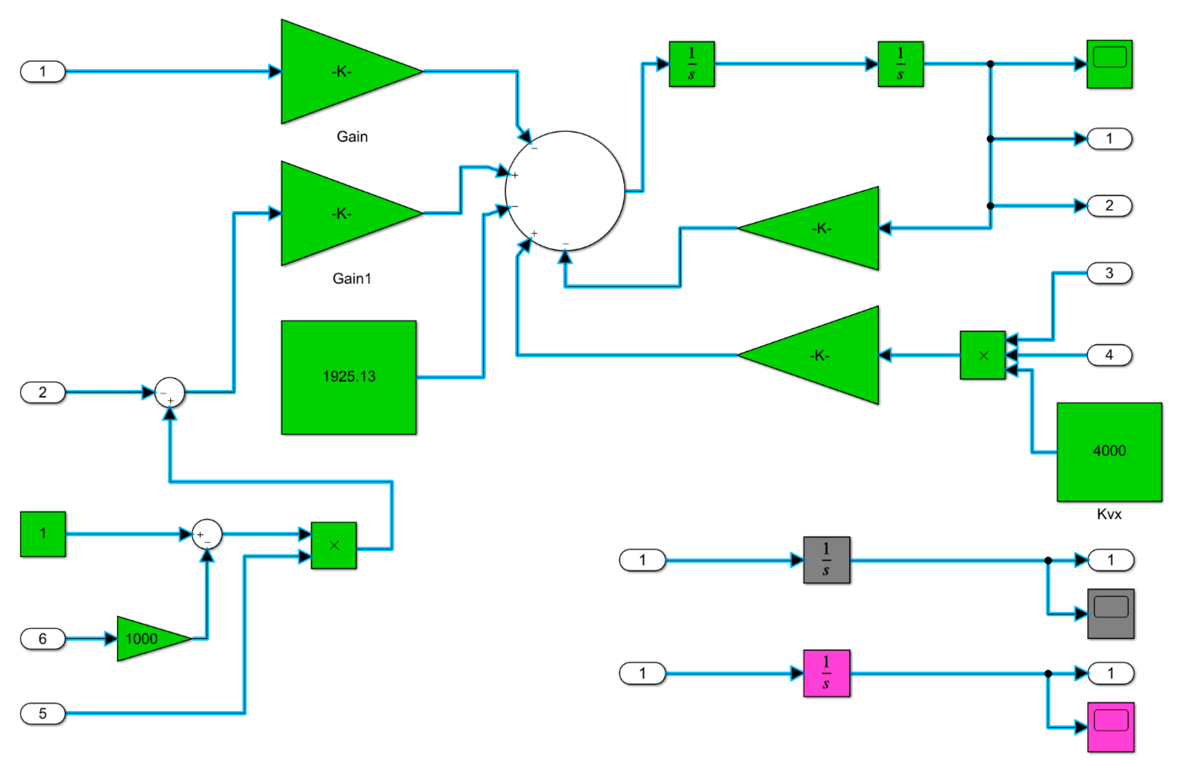
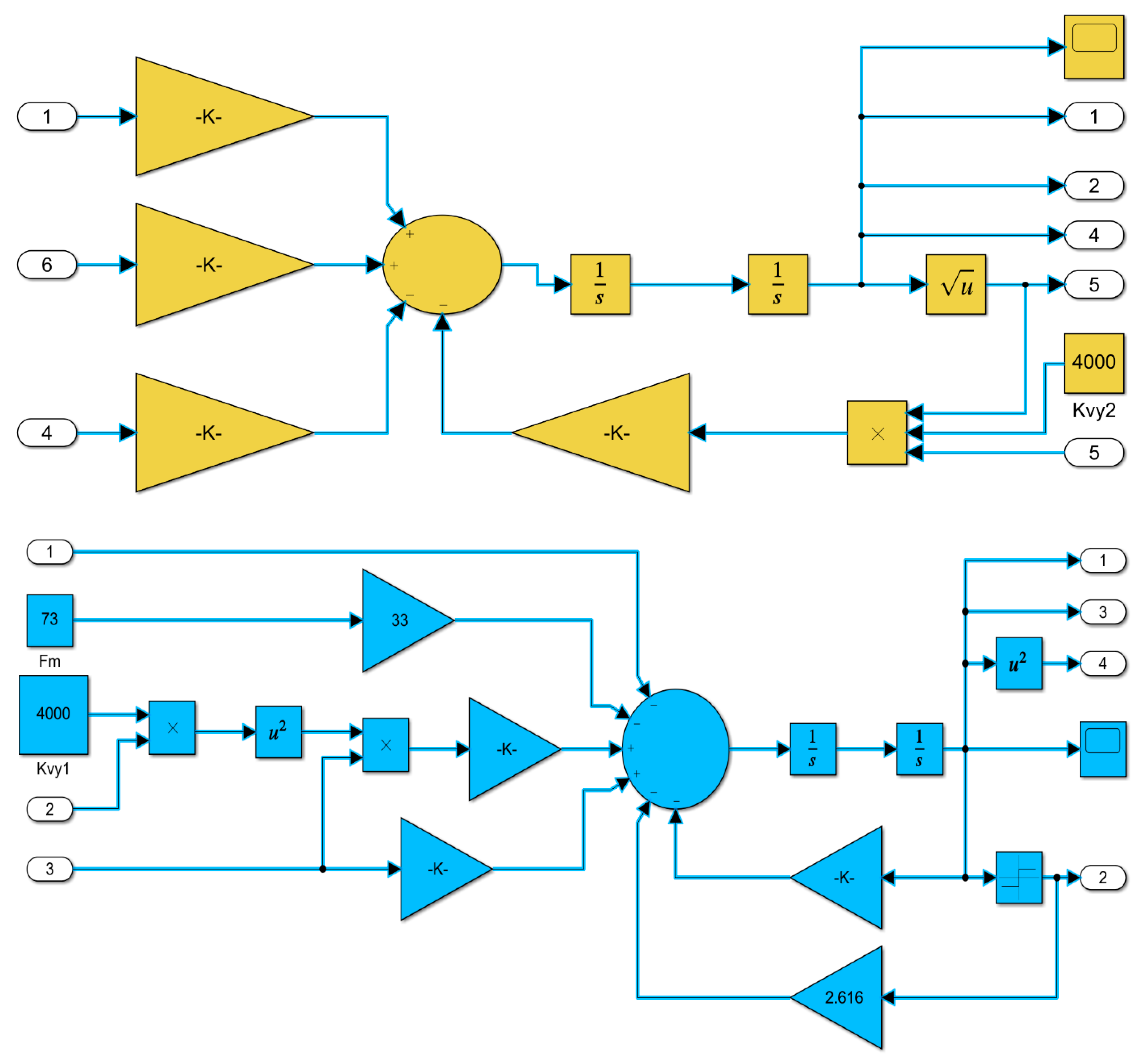
The output equations for the computer simulation of the operation of the hydraulic part are shown in Appendix A.

3. Methodology of Multi-Valued Logic Trees with Weight Coefficients as Discrete Optimization

The methodology presented is based on two algorithms:

• The Quine–McCluskey method of minimizing partial multi-valued logical functions,
• The Quine–McCluskey method of minimising partial multi-valued logical functions with multi-valued weighting factors.

3.1. Quine-Mc Cluskey Algorithm for the Minimization of Partial Multi-Valued Logical Functions

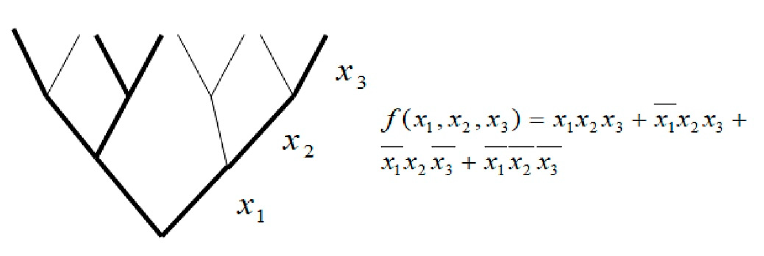
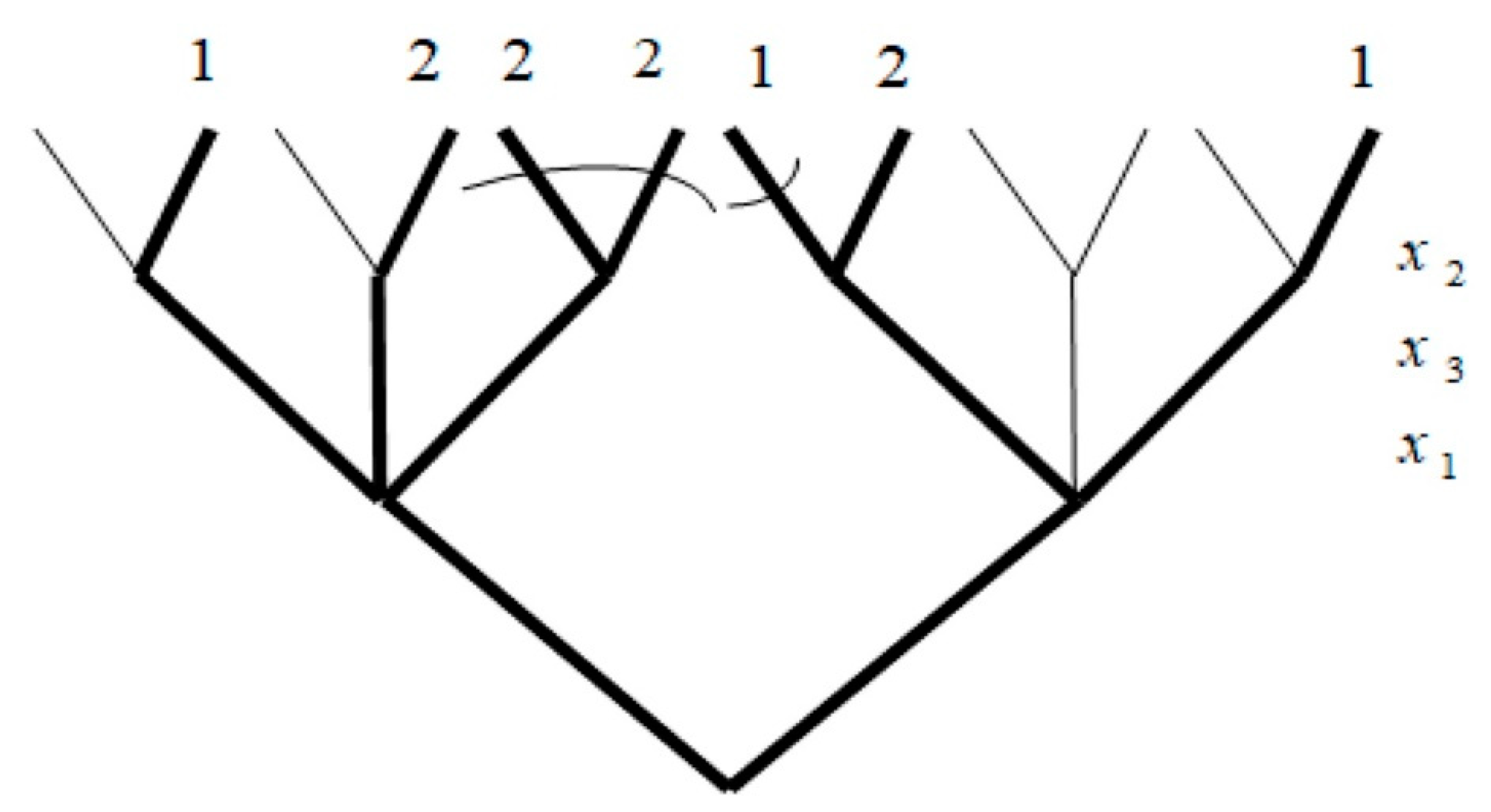
In the case of logic trees, the logical values of the variables are encoded on the branches of the tree. There can only be one Boolean variable per level of the tree, with the number of floors being equal to the number of independent variables of a given Boolean function. Representing a given Boolean function written in canonical alternative normal form (KAPN) on a logic tree involves encoding the individual canonical products on a tree path from the root to the end vertex. An individual path on the tree (from root to vertex) is a component of the singularity of the logical function, describing the realization of one possible solution. On the contrary, the set of paths is the set of all possible solutions. Figure 4 shows a logic tree in which a fixed Boolean function of three variables is encoded.

In the Quine–McCluskey algorithm, a truncated alternative normal form (SAPN) and eventually a minimum alternative normal form (MAPN) are obtained by simplifying the Boolean functions encoded in KAPN (Figure 5).

A minimized form of the output function (with a minimum number of literals) is subsequently obtained. However, given that so-called isolated branches exit, this is not the minimum decision form, meaning that there is no continuity between the root and the vertices. In the case of multi-valued logical functions—as in Boolean functions—the notions of incomplete gluing and elementary absorption, which are applied to the APN of a given logical function, play a fundamental role in the search for prime implicants.

A gluing operation is called a transformation:

$$A{j}_o\left(x_r\right)+ \dots +A{j}_{m_r-1}\left(x_r\right)=A.$$

(37)

where $r=1, \dots , n$ and $A$ denotes an elementary partial product, of which, variables of the individual literals belong to the set $\left\{x_1,\dots ,x_{r-i},x_{r+i},\dots ,x_n\right\}$.

An incomplete gluing operation is called a transformation:

$$A{j}_o\left(x_r\right)+ \dots +A{j}_{m_r-1}\left(x_r\right)=A+A{j}_o\left(x_r\right)+ \dots +A{j}_{m_r-1}\left(x_r\right),$$

(38)

where $r=1, \dots , n$ and $A$ denotes a partial product of which the variables of the individual literals belong to a set of $\left\{x_1,\dots ,x_{r-i},x_{r+i},\dots ,x_n\right\}$.

An elementary absorption operation is called a transformation:

$$A{j}_u\left(x_r\right)+A=A,$$

(39)

where $0\le u\le m_r-1, 1\le r\le n,$ and $A$ denotes a partial product of which the variables of the individual literals belong to a set of $\left\{x_1, \dots , x_{r-1}, x_{r+1},\dots , x_n\right\}$. If the above equation holds, then A absorbs $A{j}_u\left(x_r\right)$. Signs (v) denote that a given partial product of the elementary, written using the digits of the system $\left(m_1, \dots ,m_n\right)$-positional, takes part in the gluing with those products that have a sign (v) in the same column. The notation marks of the gluing operation are entered separately in the columns and not in a single column as was the case in previous literature studies of bivalent cases. In the case of equal, multivalued variables $x_1, \dots , x_n$ of a given logical function, the set of first implicants is obtained as a special case from different multi-valued variables.

Example 1.

Using the relationship:

$$A{j}_0\left(x_r\right)+ \dots +A{j}_{m-1}\left(x_r\right)=A, A{j}_u\left(x_r\right)+A=A,$$

(40)

where$A=A\left(x_1,\dots ,x_{r-1},x_{r+1},\dots ,x_n\right)$,

$$j_u\left(x_r\right)=\left\{\begin{array}{cccc}m-1& ,& u=x_r& \\ & & & 0\le u\le m-1\\ 0& ,& u\ne x_r& \end{array}\right.;$$

(41)

The successive steps of minimizing a multi-valued logical function can be represented as follows:

0	2	0					0	2	-
1	0	1					2	0	-
2	0	0					1	-	1
0	2	1					2	1	-
1	1	1					-	2	1
2	0	1					2	-	1
2	1	0
0	2	2
1	2	1
2	0	2
2	1	1
2	1	2
2	2	1
		020		200	101	021		201	210		111	022	121	202	211	212	221
02-		∗				∗						∗
20-				∗				∗						∗
1-1					∗						∗		∗
21-									∗						∗	∗
-21						∗							∗				∗
2-1								∗							∗		∗

Finally, two NAPNs and MAPNs of a given logic function are obtained, written using m-position system numbers: {(02-), (20-), (1-1), (21-), (-21)} and {(02-), (20-), (1-1), (21-), (2-1)}.

The rank of importance of successive decision variables is determined using complex alternative normal forms through the swapping of floors in logical decision trees. The swapping of logical tree floors in complex, multi-valued logical functions establishes the rank of importance of logical variables from the most important (at the root) to the least important (at the top). There is a generalization of a bivariate quality indicator to a multivariate one; (C_k − k_im_i) + (k_i + K_i), where C_k represents the number of branches of the k-th floor, k_i is the simplification factor on the k-th floor of the m_i-value variable, and K_i represents the number of branches (k − 1)-th floors from which the non-simplifying branches of the k-th floor are formed. In this way, it is possible to obtain the minimum complexity alternative normal form (MZAPN) of a given logical function without isolated branches on the decision tree and with a concomitant minimum number of real (realizable) branches, which in particular can be considered to be elementary design guidelines. All transformations refer to the so-called Quine—McCluskey algorithm for minimising individual partial multi-valued logical functions.

Example 2.

A multi-valued logical function f(x₁, x₂, x₃), where x₁, x₂and x₃are 0, 1 and 2, respectively; with a numerically recorded KAPN: 100, 010, 002, 020, 101, 110, 021, 102, 210, 111, 201, 120, 022, 112, 211, 121, 212, 221 and 122; and with one MZAPN after applying the Quine—McCluskey algorithm for minimising individual partial multi-valued logical functions has 13 literals:

$$\begin{array}{l}f\left(x_1,x_2,x_3\right)=j_o\left(x_1\right)\left(j_o\left(x_2\right)j_2\left(x_3\right)+j_1\left(x_2\right)j_o\left(x_3\right) +j_2\left(x_2\right)\right)+\\ \hspace{1em}\hspace{1em}\hspace{1em}\hspace{1em}+j_1\left(x_1\right)+j_2\left(x_1\right)\left(j_o\left(x_2\right)j_1\left(x_3\right)+j_1\left(x_2\right) +j_2\left(x_2\right)j_1\left(x_3\right)\right).\end{array}$$

(42)

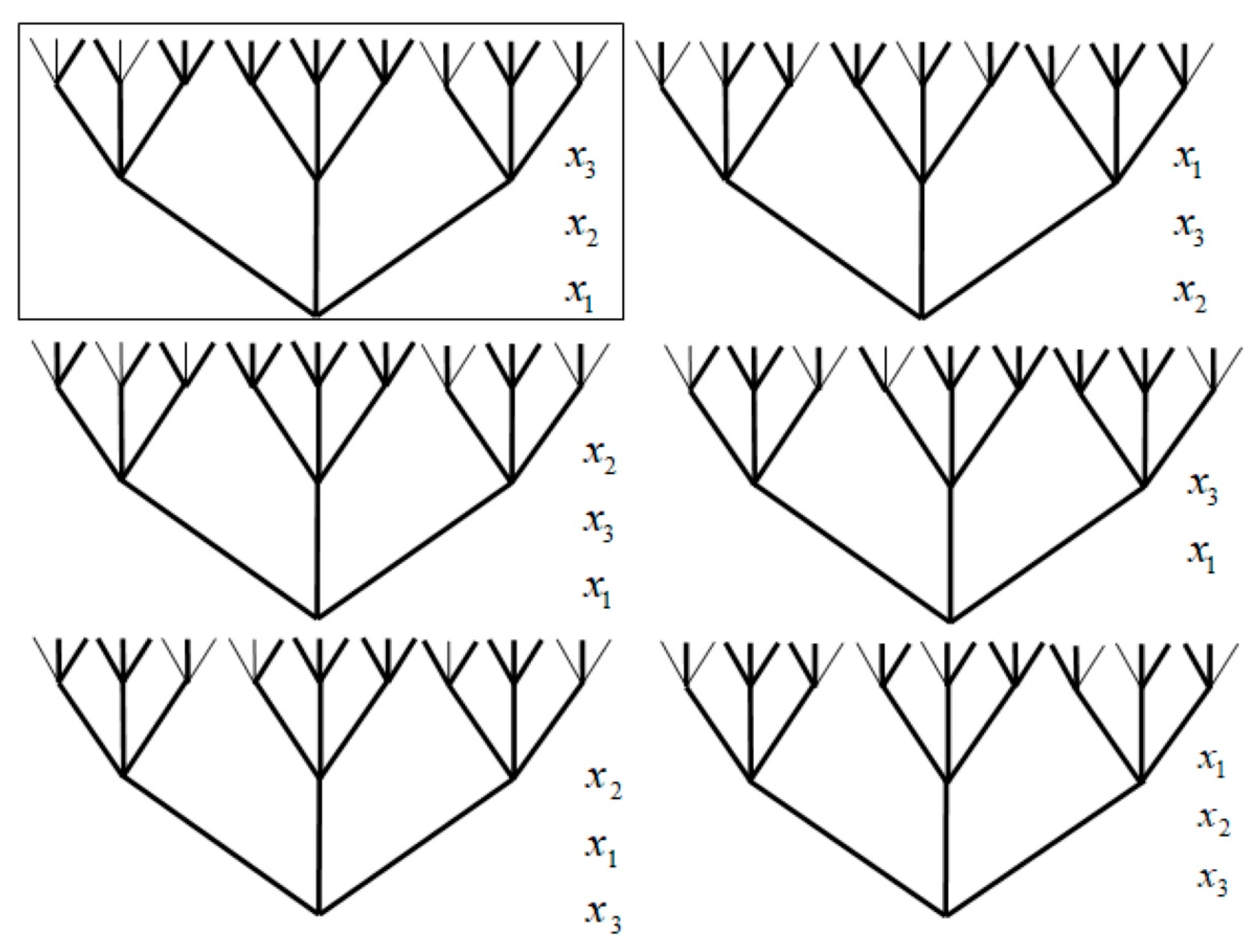
Figure 6 shows all possible ZKAPNs of a given multi-valued logical function.

• The first stage of minimization due to x₃:

		V
x1	x2	x3
1	0	0		V
0	1	0						V
0	0	2							V
0	2	0	V
1	0	1		V
1	1	0			V
0	2	1	V
1	0	2		V
2	1	0					V
1	1	1			V
2	0	1								V
1	2	0				V
0	2	2	V
1	1	2			V
2	1	1					V
1	2	1				V
2	1	2					V
2	2	1									V
1	2	2				V

2.

The first stage of minimization due to x₁:

v
x1	x2	x3
1	0	0			V
0	1	0	V
0	0	2				V
0	2	0					V
1	0	1						V
1	1	0	V
0	2	1		V
1	0	2				V
2	1	0	V
1	1	1							V
2	0	1						V
1	2	0					V
0	2	2								V
1	1	2									V
2	1	1							V
1	2	1		V
2	1	2									V
2	2	1		V
1	2	2								V

3.

The first stage of minimisation due to x₂:

	v
x1	x2	x3
1	0	0	V
0	1	0					V
0	0	2						V
0	2	0					V
1	0	1		V
1	1	0	V
0	2	1							V
1	0	2			V
2	1	0								V
1	1	1		V
2	0	1				V
1	2	0	V
0	2	2						V
1	1	2			V
2	1	1				V
1	2	1		V
2	1	2									V
2	2	1				V
1	2	2			V

x₁: 19 − 2 × 3 + 2 + 7 = 22

x₂: 19 − 4 × 3 + 4 + 5 = 16

x₃: 19 − 5 × 3 + 5 + 4 = 13

Further minimisation steps for other variables:

		v					v
	x1	x2					x1	x2
	0	0		V			0	0	V
-	1	0	V			-	1	0	V
	0	1		V			0	1		V
-	0	2		V		-	0	2			V
-	1	1	V			-	1	1		V
	2	0			V		2	0	V
-	2	1			V	-	2	1		V
-	1	2	V			-	1	2			V
	2	2			V		2	2			V

x₁: 9 − 0 × 3 + 0 + 3 = 12

x₂: 9 − 1 × 3 + 1 + 2 = 9

3.2. Generalization of the Quine–Mc Cluskey Algorithm for Minimization of Partial Multi-Valued Logical Functions for Multi-Valued Weighting Factors

In multi-valued logical functions with weighted products it is possible to apply the Quine–McCluskey algorithm for the minimization of multi-valued functions. As with the minimization of multi-valued logical functions without weighting coefficients, in the algorithm the elementary products are written as numbers in the corresponding positional systems. Additional elements and operations are introduced to account for the weighting coefficients.

In partial data of multi-valued logical functions $f_i\left(x_1,\dots ,x_n\right)$ n of variables $\left(m_1,\dots ,m_n\right)$, value-added gluing and pseudo-gluing operations should include weighting factors $\left(w_n,w_{n-1},w_{n-2},\dots ,w_1\right)$ assigned to the corresponding multi-valued logical products.

The Quine–McCluskey algorithm for minimizing multi-valued logical functions is built from n columns with $\left(w_1,\dots ,w_n\right)$ weighting factors.

Symbols indicating pseudo-gluing (V) and gluing (v) sequentially relative to groups of indices differing by one are placed in the columns corresponding to the values of the weighting factors for the corresponding logical products.

Given multi-valued weighting coefficients, individual (parallel) pseudo-bonding operations sequentially against groups of indices, differing by at least one, and containing at most $\left(m_i-1\right)$ elements can proceed in canonical products with different weighting coefficients.

The characters appear in different columns. In addition, they may be in columns with a corresponding coefficient $\left(w_n,w_{n-1},w_{n-2},\dots ,w_1\right)$. Therefore, the columns with $\left(w_1,\dots ,w_n\right)$ weighting coefficients introduce position numbers $p_i$, with i = 1,...,n, which is useful for calculating the quality of the minimization in further stages.

Definitions of ‘pure’ and ‘impure’ gluing are introduced for gluing operations of individual partial multi-valued logical functions with weighted coefficients.

Definition 1.

The pure gluing operation is the gluing of multi-valued canonical elementary products according to the Quine–McCluskey algorithm with the same weighting factor $w_i$.

A pure gluing operation is a transformation of:

$$w_{i}A{j}_0\left(x_r\right)+\dots +w_{i}A{j}_{m_r-1}\left(x_r\right)=w_{i}A,$$

(43)

where $r=1, \dots , n$ and $A$ represents a partial product of which the variables of the individual literals belong to a set of $\left\{x_1,\dots ,x_{r-i},x_{r+i},\dots ,x_n\right\}$. In n m-value variables, the weighting factor before the partial canonical product takes values in the interval $w_1,\dots ,w_n$, with $w_j=w_{j-1}+w_{j-2}+\dots +w_1$ and $j=2,\dots ,n$.

Definition 2.

The gluing operation according to the Quine–McCluskey algorithm of multi-valued canonical elementary products with different values of weight coefficients $\left(w_1,\dots ,w_n\right)$is impure gluing.

The impure gluing operation for multi-valued canonical elementary products is performed with respect to the weighting factor with the smallest value, i.e., $min\left\{w_1,\dots ,w_n\right\}$.

An impure bonding operation is a transformation:

$$\begin{array}{l}{w}_{o}A{j}_o\left(x_r\right)+ \dots +w_{m_r-1}A{j}_{m_r-1}\left(x_r\right)=\\ =\left(\min \left\{w_o,\dots ,w_{m_r-1}\right\}\right)\cdot A+{\displaystyle \sum _{s=i_o,\dots ,i_{m_r-2}}{w}_s\cdot A\cdot }{j}_s\left(x_r\right)\end{array}$$

(44)

where $r=1, \dots , n$, $w_s>min\left\{w_1,\dots ,w_{m_r-1}\right\}$, and $A$ denotes a partial product of which the variables of the individual literals belong to a set of $\left\{x_1,\dots ,x_{r-i},x_{r+1},\dots ,x_n\right\}$. In n$\left(m_1,\dots ,m_n\right)$-value variables, the weighting factor $w_i$ before the partial canonical product takes values in the interval $w_1,\dots ,w_n$, with $w_1$ where $j=2,\dots ,n$.

Definition 3.

An incomplete gluing operation is a transformation that retains the original records to be glued after the algorithm has been executed in the result.

Given that there is an isomorphic interpretation of logical transformations, the Quine– McCluskey algorithm for minimizing individual partial multi-valued logical functions can be considered with the weighting factors mentioned, which is important for describing the rank validity of design guidelines.

Example 3 with weighting factors.

In a partial logical function$f(x_1,x_2,x_3)$, written numerically in KAPN: 010, 100, 002, 011, 110, 012 and 112, the Quine–McCluskey algorithm for minimizing logical functions with multi-valued weight coefficients yields one MZAPN which has 11 literals of $f(x_1,x_2,x_3)$, i.e.,

$$\begin{array}{l}f(x_1,x_3,x_2)=j_0(x_1)\left(1j_0(x_3)j_1(x_2)\right)+2j_1(x_3)2j_1(x_2)+2j_2(x_3))\\ +j_1(x_1)\left(1j_2(x_3)j_1(x_2)\right)+2j_0(x_3)j_1(x_2))\end{array}$$

(45)

while other ZAPN$f(x_1,x_2,x_3)$,$f(x_2,x_1,x_3)$,$f(x_2,x_3,x_1)$and$f(x_3,x_1,x_2)$of a given logical function have 12 and$f(x_3,x_2,x_1)$13 literals, respectively.

$$\begin{array}{l}f(x_2,x_3,x_1)=j_0(x_2)\left(1j_0(x_3)j_1(x_1)+2j_2(x_3)j_0(x_1)\right)\\ +j_1(x_2)\left(2j_0(x_3)j_1(x_1)+2j_1(x_3)j_0(x_1)+2j_1(x_3)j_0(x_1)\right)\end{array}$$

(46)

$$\begin{array}{l}f(x_2,x_1,x_3)=j_0(x_2)\left(2j_0(x_1)j_2(x_3)+1j_1(x_1)j_0(x_3)\right)\\ +j_1(x_2)\left(2j_0(x_1)\left(j_1(x_3)+j_2(x_3)\right)+j_1(x_1)\left(2j_0(x_3)+1j_2(x_3)\right)\right)\end{array}$$

(47)

$$\begin{array}{l}f(x_1,x_2,x_3)=j_0(x_1)\left(2j_0(x_2)j_2(x_3)+2j_1(x_2)\left(j_1(x_3)+j_2(x_3)\right)\right)\\ +j_1(x_1)\left(1j_0(x_2)j_0(x_3)+j_1(x_2)\left(2j_0(x_3)+1j_2(x_3)\right)\right)\end{array}$$

(48)

$$\begin{array}{l}f(x_3,x_1,x_2)=j_0(x_3)\left(1j_0(x_1)j_1(x_2)+2j_1(x_1)j_1(x_2)\right)\\ +2j_1(x_3)j_0(x_1)j_1(x_2)+j_2(x_3)\left(2j_0(x_1)+1j_1(x_1)j_1(x_2)\right)\end{array}$$

(49)

$$\begin{array}{l}f(x_3,x_2,x_1)=j_0(x_3)\left(1j_0(x_2)j_1(x_1)+2j_1(x_2)j_1(x_1)\right)\\ +2j_1(x_3)j_1(x_2)j_0(x_1)+j_2(x_3)\left(2j_0(x_2)j_0(x_1)+2j_1(x_2)j_0(x_1)\right).\end{array}$$

(50)

The following are the successive steps in the minimisation of logical functions due to given decision variables:

			v
wi	x1	x2	x3	wi = 2						wi = 1
1	0	1	0							V
1	1	0	0									V
2	0	0	2				V
2	0	1	1	V						V
2	1	1	0		V
2	0	1	2	V						V
1	1	1	2								V
	pi			1	2	3	4	5	6	1	2	3	4	5	6
		v
wi	x1	x2	x3	wi = 2						wi = 1
1	0	1	0									V
1	1	0	0							V
2	0	0	2		V
2	0	1	1				V
2	1	1	0	V						V
2	0	1	2		V
1	1	1	2											V
	pi			1	2	3	4	5	6	1	2	3	4	5	6
	v
wi	x1	x2	x3	wi = 2						wi = 1
1	0	1	0								V
1	1	0	0									V
2	0	0	2				V
2	0	1	1					V
2	1	1	0		V						V
2	0	1	2	V						V
1	1	1	2							V
	pi			1	2	3	4	5	6	1	2	3	4	5	6
			V
	wi	x2	x3	wi = 2						wi = 1
2(012)	1-	1	2							V
2(110)	1-	1	0							V
	2	1	1	V
	2	0	2		V
	2	0	0		V
	pi			1	2	3	4	5	6	1	2	3	4	5	6
		V
	wi	x2	x3	wi = 2						wi = 1
2(012)	1-	1	2							V
2(110)	1-	1	0								V
	2	1	1			V
	2	0	2	V
	2	0	0		V
	pi			1	2	3	4	5	6	1	2	3	4	5	6
			V
	wi	x1	x3	wi = 2						wi = 1
	1	0	0							V
2(110)	1-	1	0								V
	2-	0	2	V
	2	0	1	V
	1	1	2								V
	pi			1	2	3	4	5	6	1	2	3	4	5	6
		V
	wi	x1	x3	wi = 2						wi = 1
	1	0	0							V
2(110)	1-	1	0							V
	2-	0	2			V
	2	0	1		V
	1	1	2									V
	pi			1	2	3	4	5	6	1	2	3	4	5	6

Tree interpretation.

Figure 7 shows the MZAPN of the multi-valued logical function from Example 3.

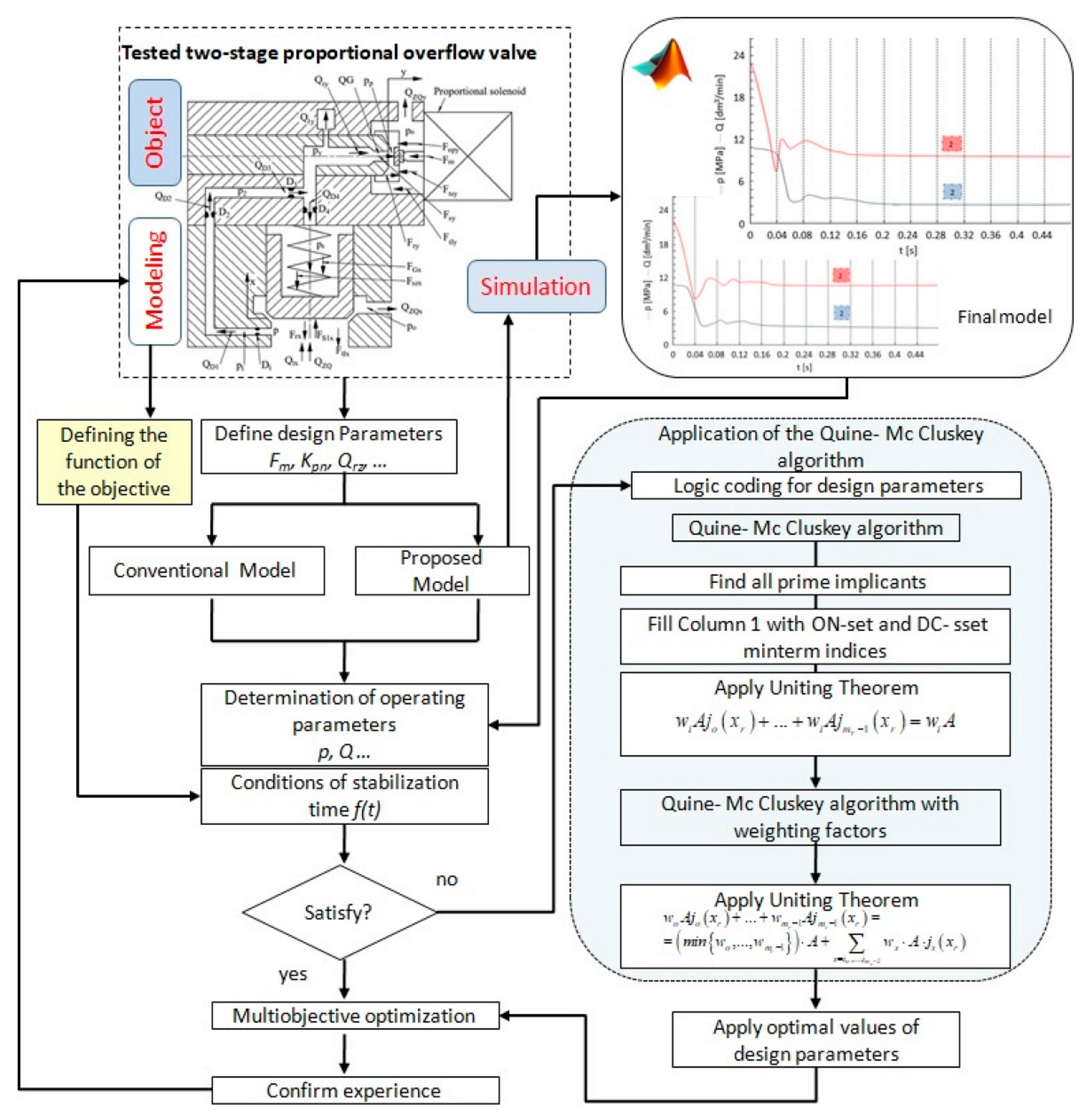
The proposed methodology can be described by the flow chart shown in Figure 8.

The structuring of the described problem takes into account the methodology of multi-valued logical trees, allowing for the introduction of appropriate formal notations and even making it possible to combine complex quantitative and qualitative features with different degrees of detail according to the principles of a multidimensional morphological array. Therefore, there is no need to extend the generation process to sub-arrays when using a multidimensional morphological array as all information about the varieties of the main and detailed features and their numerous modifications can be immediately stored in this array and marked on the variant tree.

In addition, the morphological and decision tables can be encoded analytically and numerically according to the definitions and theorems of the logic of multi-valued decision processes. This enables a variant way of identifying and classifying information in computer science terms when seeking and modifying solutions in the design process.

In such a situation it is possible to introduce CAD, e.g., for the generation of all theoretical variants of the designed system, selection for realizability, search for realizable solutions and—most importantly—realizable sub-solutions, etc. In order to ensure the stable operation of the actual system, model tests are carried out on the basis of which of the relevant parameters are selected. The phenomena occurring during the flow of a medium are quite often not precisely defined, so it is necessary to identify an analytical model when carrying out such studies.

4. Application of the Methodology of Multi-Valued Logic Trees with Weighting Factors in the Optimization of a Proportional Valve

Tests have already been carried out for valves of the direct-acting UPZ type [4], which are designed to regulate the upstream pressure of steam and non-flammable, chemically inert gases and liquids regardless of the pressure at their outlet. Multivalent weighting factors were not considered in the tested valve class. For this reason, it was decided that an improved Quine–McCluskey algorithm with weighting factors for the hydraulic proportional valve would be used. Therefore, three ‘novelties’ are presented in this paper.

One of the optimal methods presented are multi-valued logic algorithms. For example, in [24] the authors presented a description of the dynamics of molecular states caused by a sequence of laser pulses using multi-valued logic. In turn, the authors of [25] used multi-valued logical schemes to calculate significance measures based on incompletely-defined data. This method is based on the definition of a mathematical model of an analyzed system in the form of a structure function that determines the correlation of the system reliability and the states of its components.

In [27], the authors described the historical and technical background of MVL, as well as the areas of present and future applications of quadrivalent logic. It was also intended to serve as a guide for non-specialists. The wide application of multi-valued logic in particular in these microelectronic circuits is presented in [28]. Additionally, there are many original works describing the practical application of multi-valued logic trees.

In addition, there are other works in which multi-valued decision trees and logic algorithms have been applied. For example, the authors of [29] presented the applications of machine learning and classification and regression trees (CART) in medicine. Specifically, they presented the concept of a gradient-boosting algorithm. The authors of [30] presented the application of a rotation forest with decision trees as a base classifier and a new ensemble model in the spatial modeling of groundwater potential. The use of fault-tree analysis to calculate system-failure probability bounds from qualitative data in an intuitive, fuzzy environment is presented in paper [31]. Meanwhile, in paper [32] the authors adopted component fault trees (CFTs) to support fault tree analysis, failure mode, and effect analysis as extensions of SysML models. Boolean decision support methods were presented in paper [33]. A very modern optimization method was proposed by the authors of [34]: the use of root trees. The root-tree algorithm was used for high-order sliding mode control using a super-twist algorithm based on the DTC scheme for DFIG.

The initial conditions of a differential equation can be determined by entering $\frac{d{x}_i}{dt}=0$. The simulations were performed using the Matlab/Simulink package:

$$\left\{\begin{array}{l}-801.2102\cdot {10}^{-3}(k_{vx}{x}_1)x_3-147224.3x_1-1925.135+5.3792244\cdot {10}^{-3}\left[(1-{10}^3{x}_1)x_3-x_6\right]=0,\\ 0.2851216\cdot {10}^9(1-1.32\cdot {10}^{-9}{x}_3)-0.5279061\cdot {10}^9(k_{vx}{x}_1)\sqrt{x_3}-7.65(x_3-x_6)-0.3227777\cdot {10}^{12}{Q}_{odb}=0,\\ 0.7123874\cdot {10}^{-4}{x}_7+418.87733{(k_{vy}{x}_4)}^2{x}_7-33.33333F_m=0,\\ 0.276556\cdot {10}^5(x_3-x_6)-0.312234\cdot {10}^{12}(k_{vy}{x}_4)\sqrt{x_6}=0,\\ x_7=x_6-0.2025169\cdot {10}^6(k_{vy}{x}_4)\sqrt{x_6}.\end{array}\right.$$

(51)

Assuming that:

$$U_z=U_p=1 V.$$

(52)

It can be obtained that:

$$\begin{array}{l}{U}_z=U_p=1 V,\\ Q_{odb}=12/6\cdot {10}^{-4}\left[\frac{m^3}{s}\right].\end{array}$$

(53)

The Importance of the Design and/or Operational Parameters of a Hydraulic Proportional Valve

In the optimization process, the changed parameters of the proportional valve while observing the Q flow rate and p pressure are represented by the regulator K_p1·K_p2 gain (as a complex variable), the Q_obd receiver flow rate (depending on the impulse input of the U_z control voltage), and the F_m magnetic force.

The arithmetic values of the tested parameters were selected for the analysis. They were coded by the authors of this work with logical decision variables:

$$\begin{array}{l}(K_{p1}\cdot K_{p2})=30\sim 0;\\ (K_{p1}\cdot K_{p2})=40\sim 1;\\ (K_{p1}\cdot K_{p2})=50\sim 2;\\ (K_{p1}\cdot K_{p2})=60\sim 3;\\ F_m=1.96\left[\mathrm{N}\right]\sim 0;\\ F_m=2.96\left[\mathrm{N}\right]\sim 1;\\ F_m=3.96\left[\mathrm{N}\right]\sim 2;\\ F_m=4.96\left[\mathrm{N}\right]\sim 3;\\ Q_{rz}=36\to 24\left[{\mathrm{dm}}^3/\min \right]\sim 0;\\ Q_{rz}=24\to 12\left[{\mathrm{dm}}^3/\min \right]\sim 1;\\ Q_{rz}=36\to 12\left[{\mathrm{dm}}^3/\min \right]\sim 2;\end{array}$$

(54)

In the operation of the relief valve, the authors introduced restrictions on the Q and p design parameters in terms of the stabilization time t_w:t_w < 0.48 t₀. Subsequently, dynamic calculations of the valve were carried out, resulting in the t_w:t_w < 0.48 t₀ limitation. Following the dynamic calculations, 23 charts were selected. The code changes of the K_p1, K_p2, Q_rz and F_m design parameters are presented in

Table 1. KAPN for the K_p1, K_p2, Q_rz and F_m parameter code data, taking into account the w_i weighting factors.

wi	Fm	Kp1, Kp2	Qrz
2	2	1	2
2	2	3	2
2	2	2	1
2	2	2	2
2	1	2	1
3	3	0	2
1	1	0	2
2	0	2	1
1	0	2	2
2	0	2	0
3	0	3	1
2	0	3	2
3	0	1	1
1	0	1	2
3	0	1	0
2	0	0	1
1	0	0	2
1	1	2	2
2	1	1	2
1	1	3	2
1	3	2	2
1	3	1	2
3	3	3	2

.

Furthermore, in the code changes of the K_p1·K_p2, Q_rz and F_m design parameters multi-valued w_i weighting factors are introduced, similar to the relief valve. The greater the weighting number, the faster the Q and p functions reach a stable state (t_t > t_j).

The following weighting factors were adopted in the t_w < 0.48 t₀ limitation:

• w_i = 3, t_w ≤ 0.16 t₀;
• w_i = 2, 0.16 t₀ < t_w ≤ 0.32 t₀;
• w_i = 1, 0.32 t₀ < t_w ≤ 0.48 t₀.

Table 1 presents the code changes of the K_p1·K_p2, Q_rz and F_m design parameters, taking into account the multi-valued weighting factors and the t_w < 0.48 t₀ limitation.

Notably, the value of the weighting factor for changes in the code K_p1·K_p2, Q_rz and F_m design parameters in Table 1 is minimal among the coefficients defined separately in the Q and p function. If one of the functions stabilizes faster than the other, then the canonical product for the same code changes of K_p1·K_p2, Q_rz and F_m parameters should be assigned a smaller weighting factor.

In the system of multi-valued logic functions with weighting factors, weighting factors are assigned separately for each of the functions.

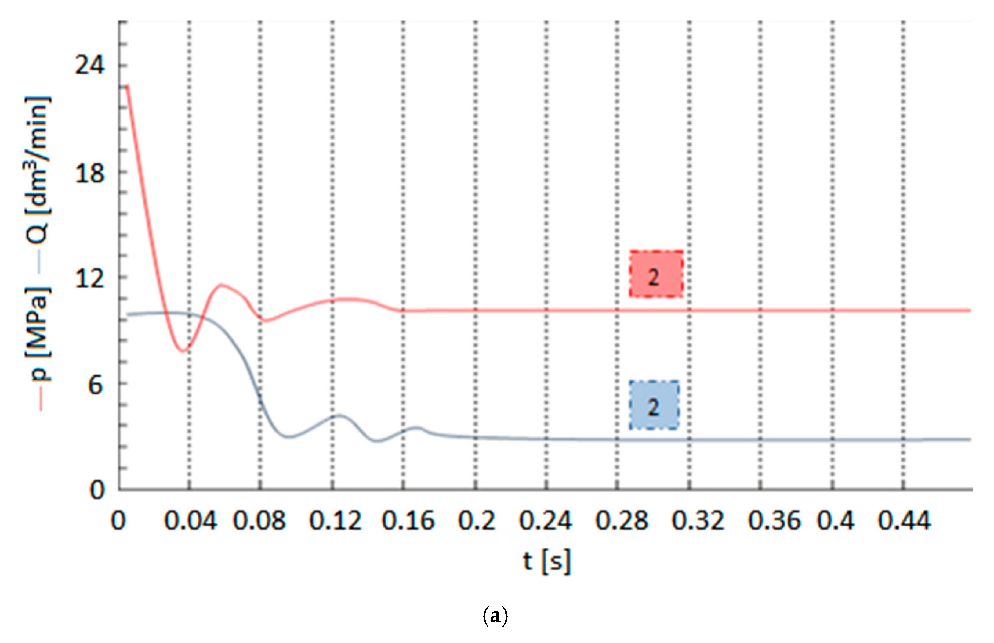
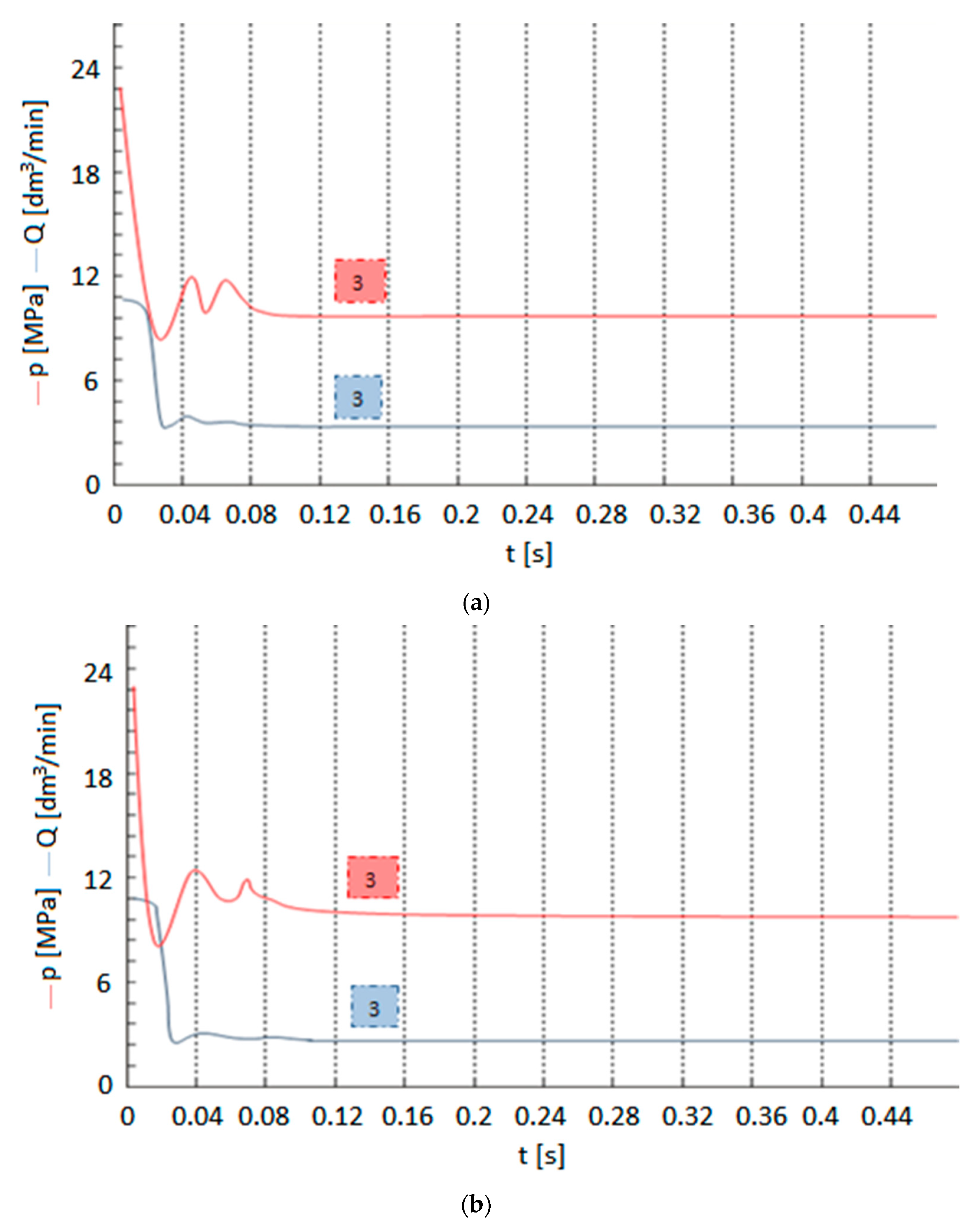
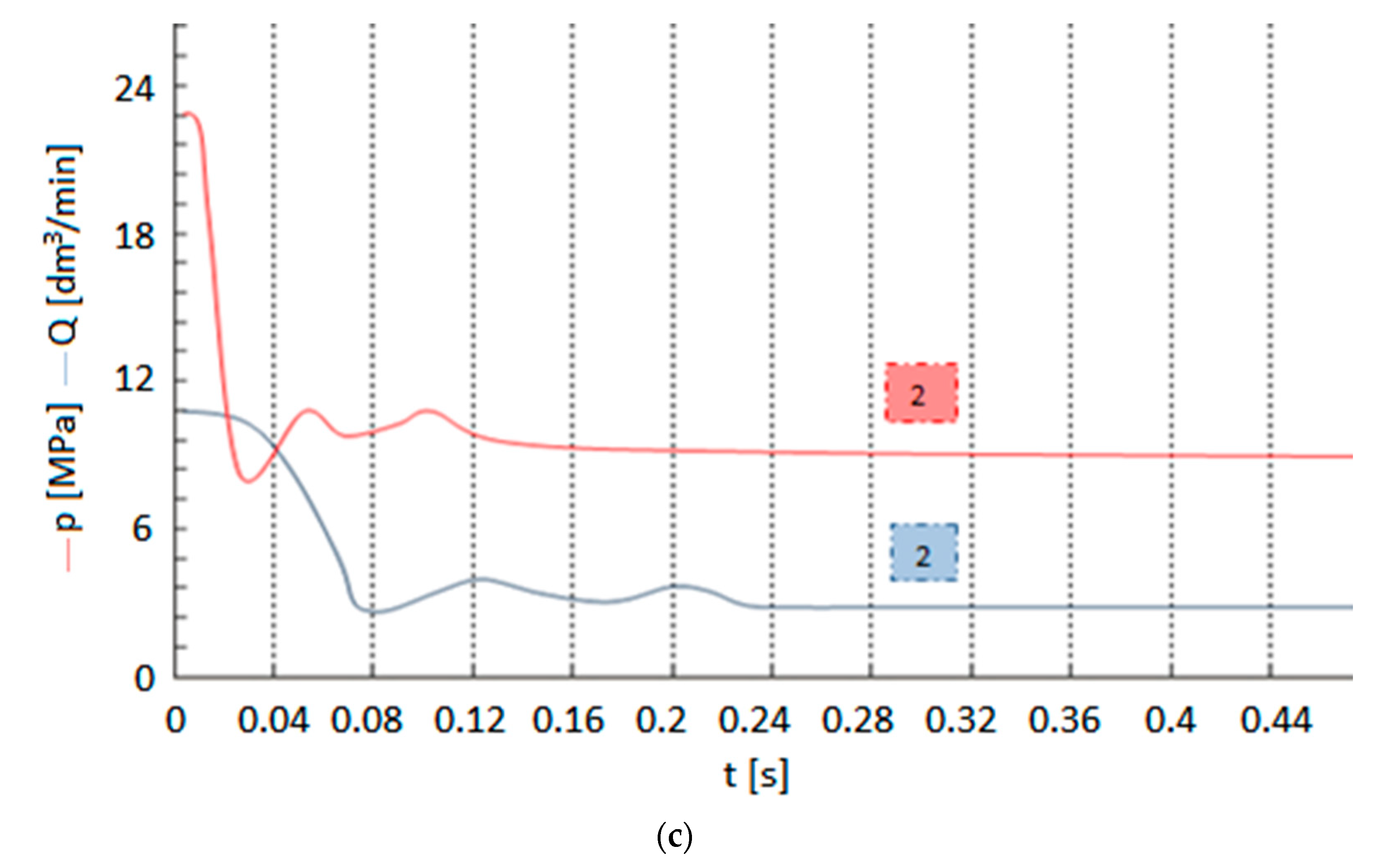
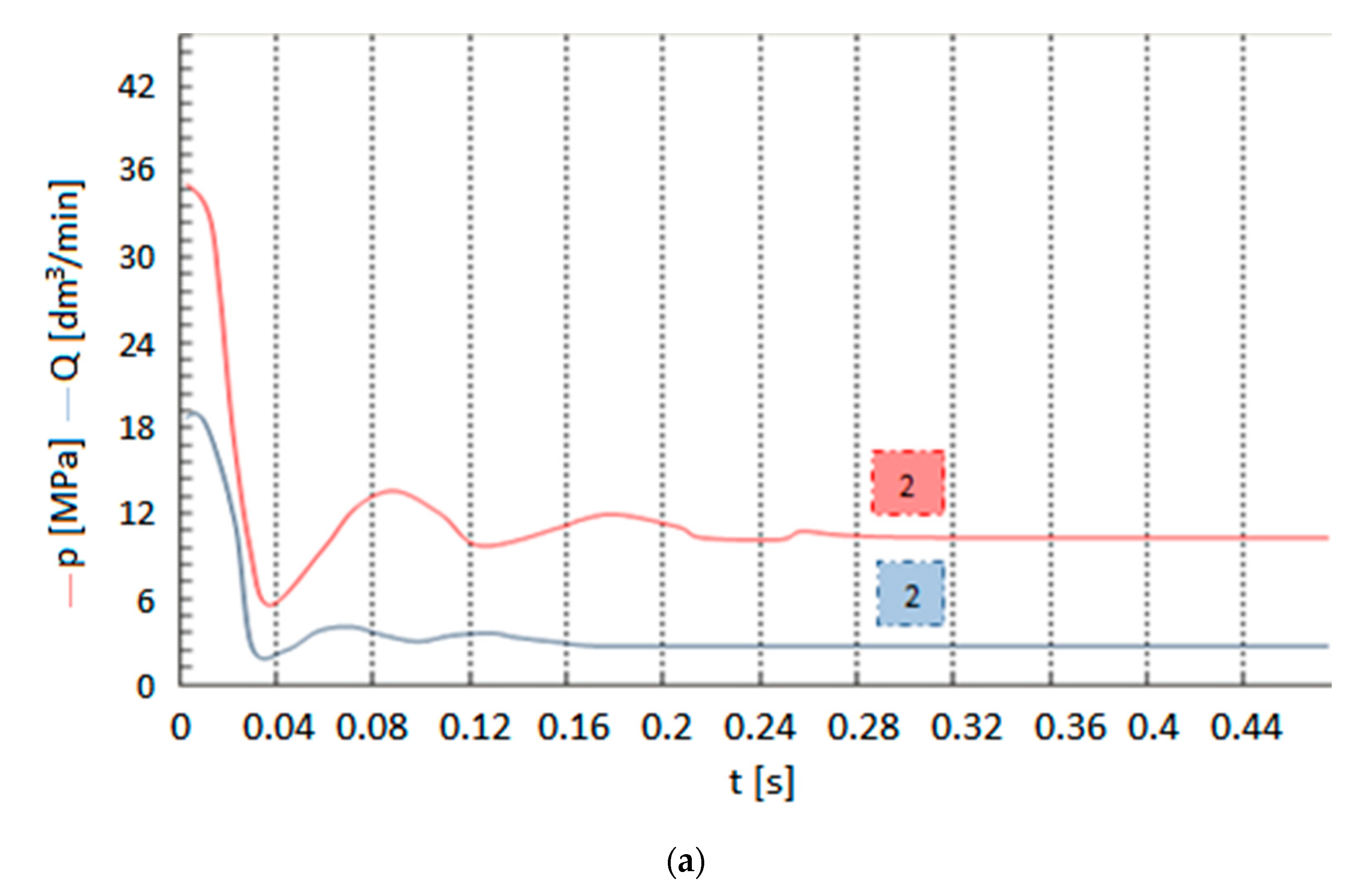
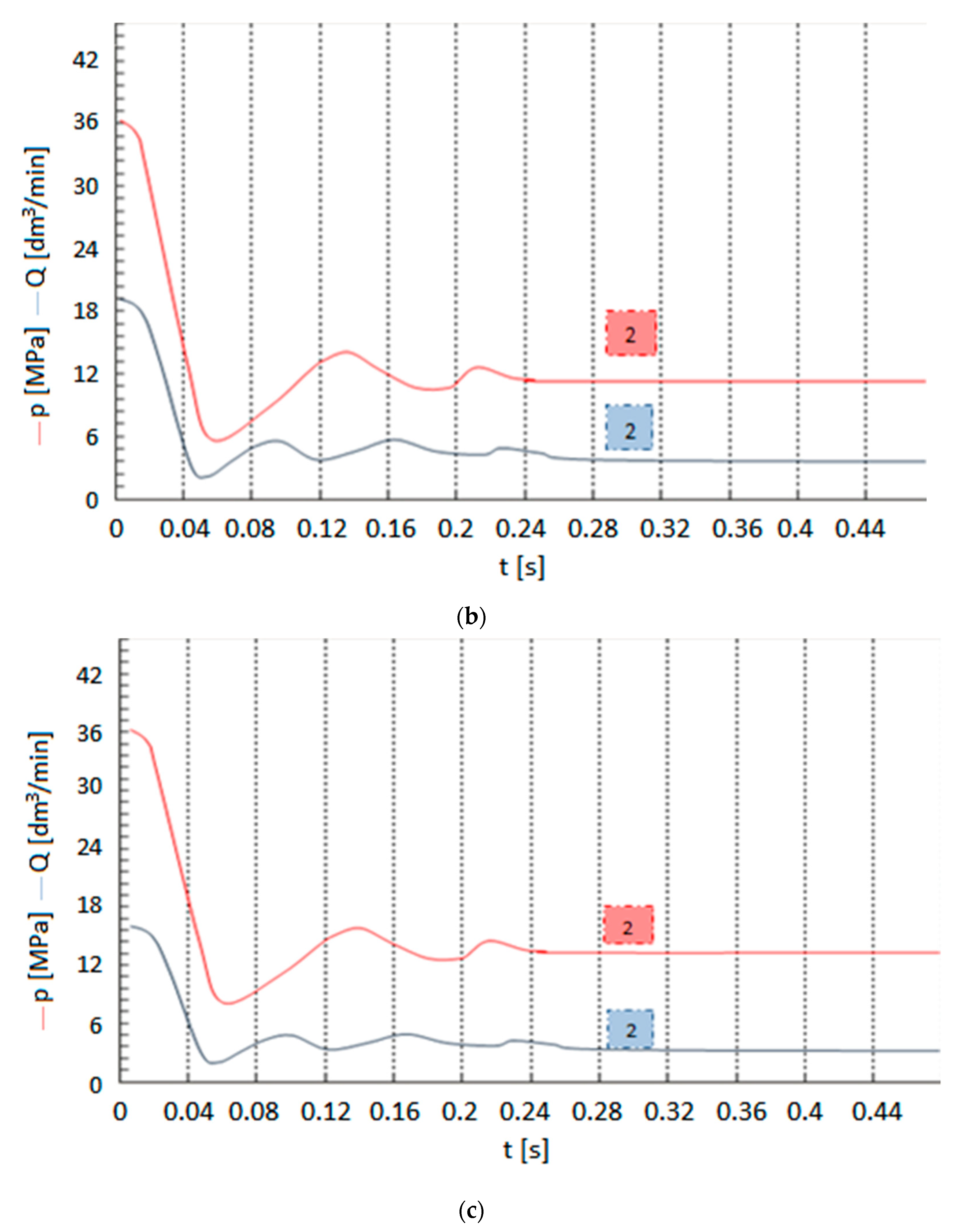
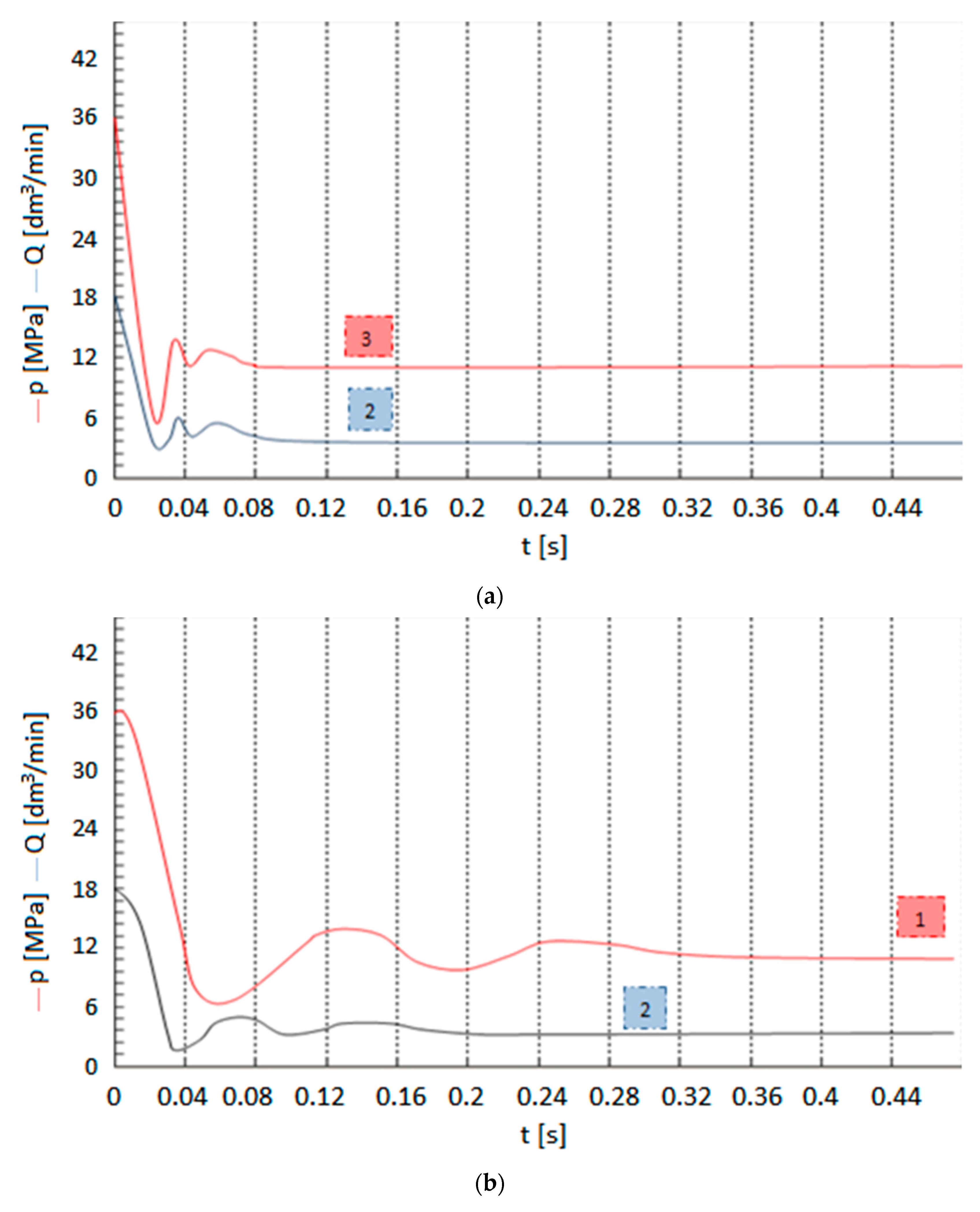
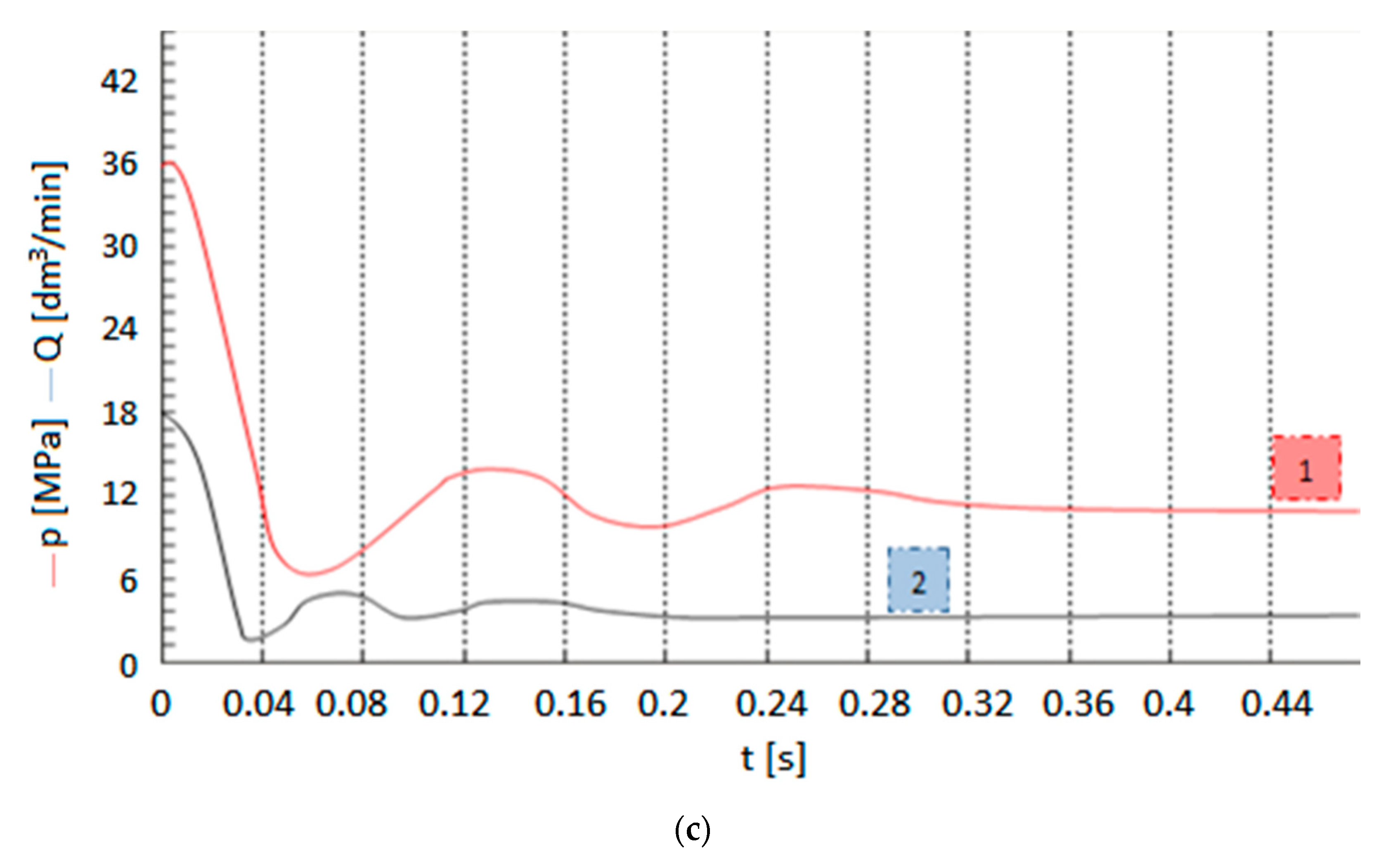
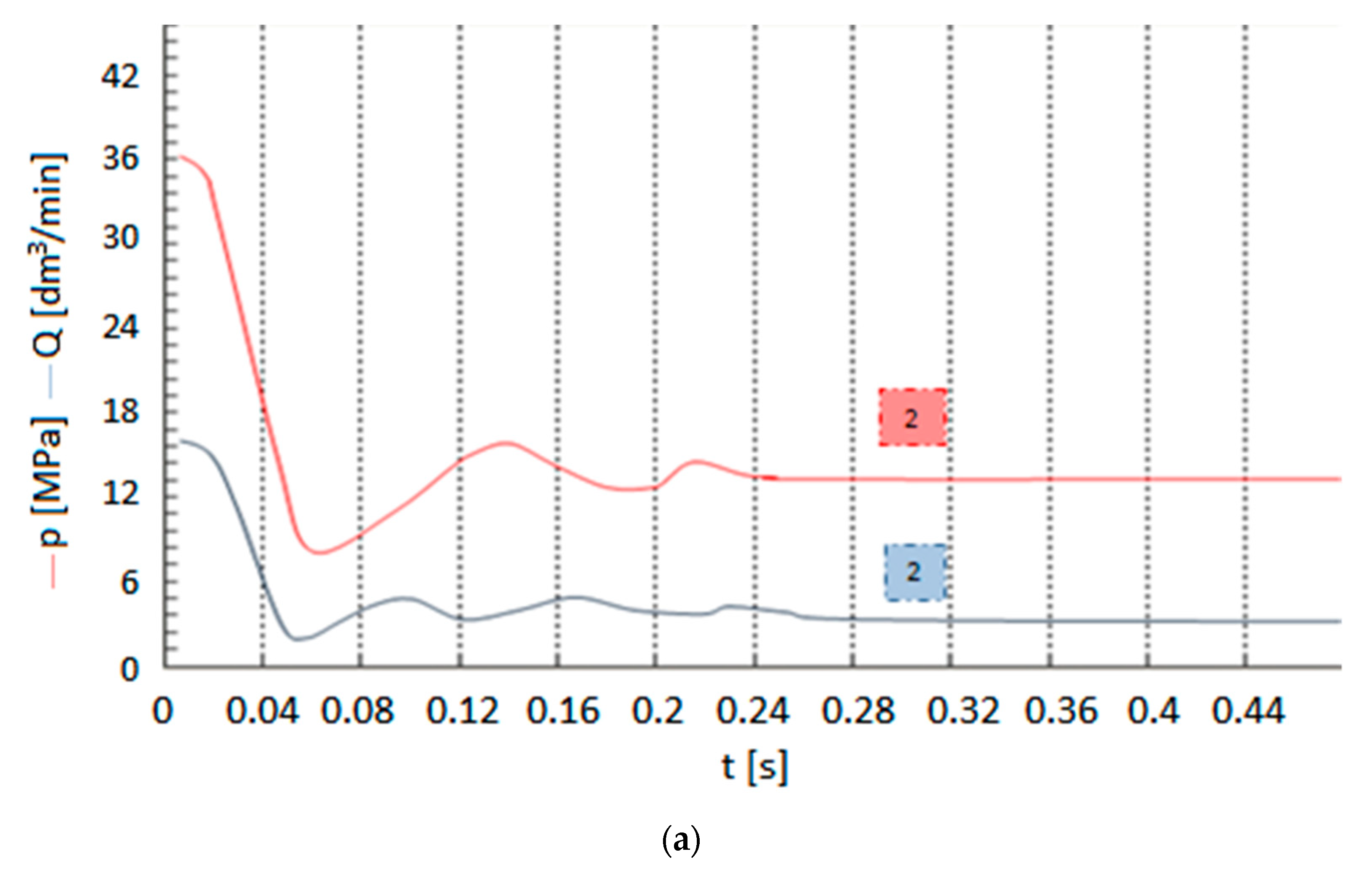
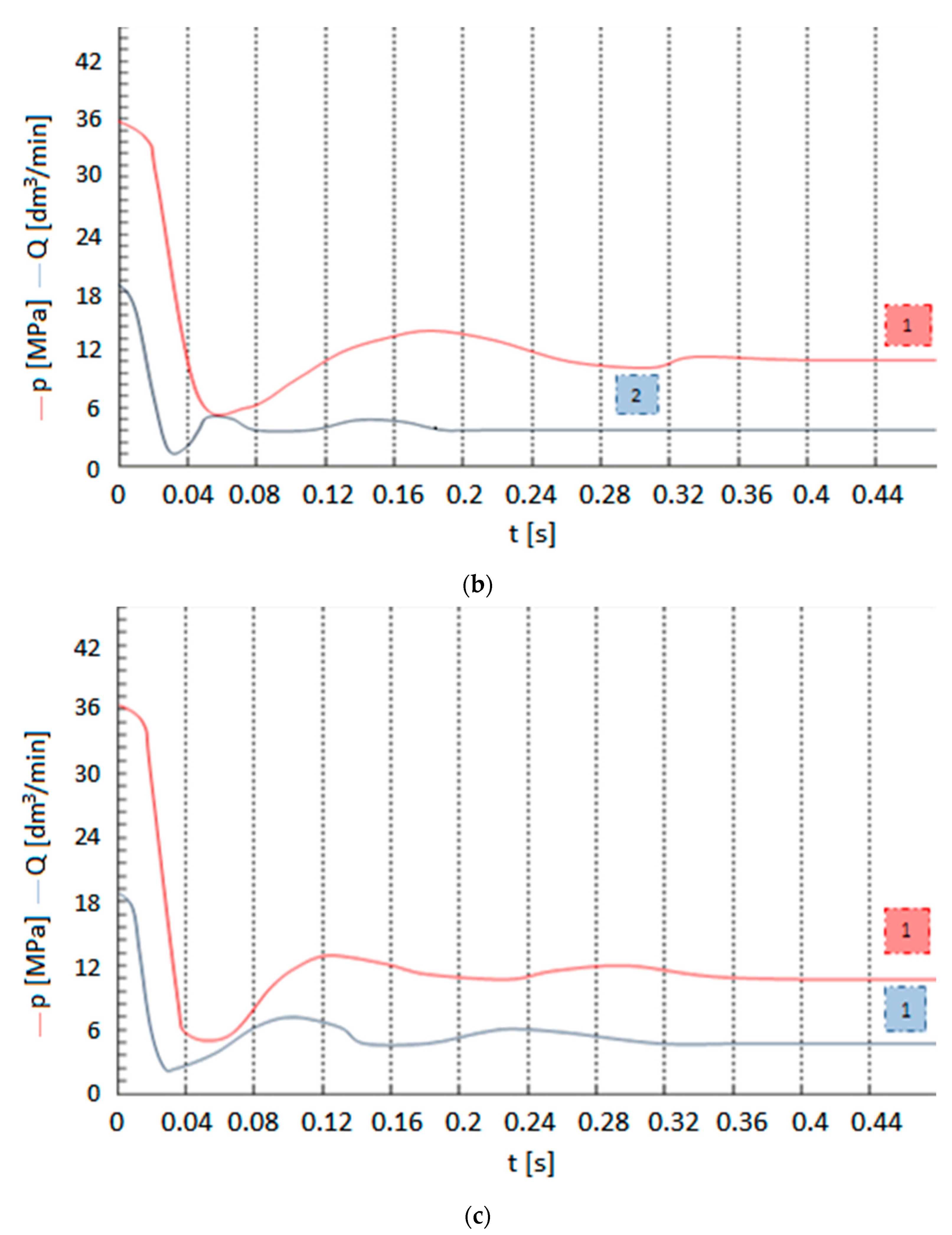
Figure 9, Figure 10, Figure 11, Figure 12 and Figure 13 show the time periods of the Q and p functions with the weighting factor intervals marked w_i:p (red color) and Q (blue color).

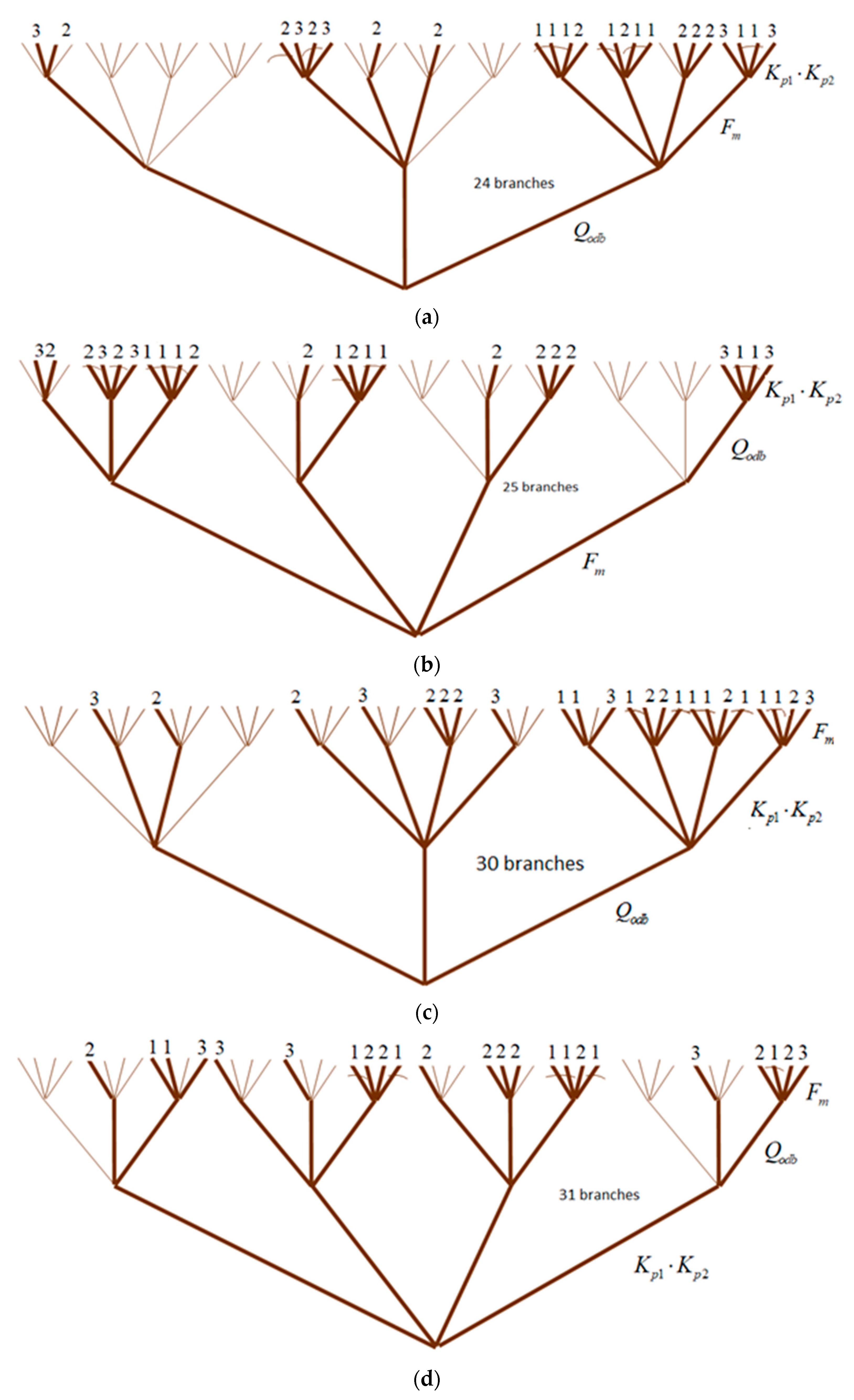
The multi-valued logical trees with the weighting factors from Table 1 are shown in Figure 14.

For the t_w < 0.48 t₀ criterion of limitation, one optimal multi-valued logical tree is presented in Figure 14. For a hydraulic proportional valve, the most crucial parameter is the Q_odb flow rate of the receiver (depending on the U_z step function of the control voltage).

One of the issues presented in this paper is the application of Boolean equations in the optimization of machine systems. This paper generalizes the Quine–McCluskey algorithm for minimizing multi-valued logical functions with multi-valued weight coefficients. In addition, a procedure for the combinatorial solution of weighted multi-valued systems of logical equations describing design guidelines in terms of morphological analysis with the Rosser–Turguette axioms is discussed.

The application of the methodology of multi-valued logic trees with weighting coefficients for relief valves allows for the determination of alternative sets of design guidelines to find the most crucial design guidelines in any fixed design and/or operational parameters while ensuring that the constraints and extremes of the criterion are met. In particular, the novelty presented in this paper is:

• the development of a Quine–McCluskey algorithm for minimizing logical functions with weighted coefficients;
• the development of algorithms for multi-valued Boolean equations, allowing for the obtainment of the most important design guidelines in the process of optimization of machine systems; and
• carrying out calculations on a real object (relief valve) to confirm the developed algorithms.

5. Conclusions

This paper presents the use of multi-valued logical trees with weighting factors to determine the importance of the constructional and operational parameters of a two-stage proportional relief valve. As has been demonstrated by this research, relief valves do not keep up with a pressure increase in the system, react with a certain delay, and can vibrate under fixed operating conditions.

The above incorrect response of the valves usually occurs during the transition period. Hence, it is necessary to carry out model tests of valves in the transition state and to determine the importance of the operational parameters directly affecting their dynamics. Model tests aim to select essential parameters to ensure the stability of the real system. It is crucial to determine the importance of design and/or operational parameters during the model verification and subsequently select the appropriate optimization procedure.

This work discusses the procedure of a combinatorial solution for weight–multi-valued systems of logic equations describing the design guidelines in terms of morphological analysis with the preservation of Rosser–Turguette axioms. It has been shown that, in general, the minimization of logic functions with weight coefficients may be the same as without weight coefficients. However, a better reflection of the physical models of hydraulic relief systems was obtained through mathematical models. The literature shows that various coefficients of logical products have not been taken into account in the separable and common minimization of systems of multi-valued logic equations.

Three following ‘novelties’ are presented in this paper:

• The Quine–McCluskey algorithm was applied to completely new proportional valves previously not tested using such methods;
• Multivariate weighting factors were taken into account, which allowed for the introduction of multi-valued weighting factors to determine the most important design guidelines. This made it possible to apply the method of multi-valued decision trees to solve the technological problems of the studied proportional valve series. It also made it possible to use systems of logical equations as a formal decision-making description of the study of the importance rank of changes in design and operating parameters as a method for optimizing relief valves and other hydraulic systems;
• For the optimization process of hydraulic valve design, an approach using CFD computer simulation methods is encountered. However, any results obtained from simulation solutions should be, at least to some extent, verified by reliable experimental studies.

Limits of the Methodology Used

Each of the KAPN products should be assigned corresponding discrete changes in parameter values. Therefore, it is not possible to fully apply the developed methods in continuous linear and non-linear optimisation. However, for construction/engineering purposes, the use of discrete analysis is preferable in the opinion of the authors (who have computational experience). If one were to change the numerical values of the input variables in a mathematical model, one would obtain changes in the values of the output variables. In order to obtain a different planned behaviour of a system (component), one can often make many changes to the numerical values of the input variables. Concerns related to change include: which values might be changed, how the change might be made (by increasing values, keeping them unchanged, or decreasing them), or in what order the variables might be changed, etc. Such conjecturing is akin to subjectively (according to a given designer) changing the numerical values in a mathematical model. This means that another designer, according to their own experience, may subjectively redesign the layout (element) quite differently for new work conditions that are identical to those of the previous designer.

The multi-valued weighting system of logical equations describing the design guidelines can be minimized separately or together with logical equivalence. Still, even in the bivalent (Boolean) case, the common minimization is not inferior to the separate minimization in terms of literal multiplicity. Increasing, reducing, or keeping the numerical values unchanged in the process of redesigning a system for other operating conditions can be coded using multi-valued logic while sets of design guidelines can be presented as sums of multi-valued logical products.

Model tests are particularly important in the design of new valves. These design parameters, which significantly affect the dynamics of valves, cannot be selected randomly (depending on the assumptions and experience of the designer). Their values should be closely related to the permissible peak overload of the controlled signal, operation speed, time constant, and eliminating vibration. Model tests will be more useful if the described valve is outlined more accurately in the transition state. Thus, building a correct analytical equation that presents a given valve in a dynamic course determines the sense of any theoretical considerations.

In further research, it will also be necessary to take into account the modified methodology of multi-valued logic trees as parametrically-playing out graphs, i.e., a heuristic simulation method for solving linear–dynamic decision models for relief valves. In the instance analyzed, a number of simplifications were additionally taken into account; for example, the impact of the closing element hitting the valve seat was not considered and the effect of the valve-wall compressibility was not taken into account. These factors will be considered in further papers. Additionally, a new control system using optimised proportional–directional control valves, throttling valves, and flow controllers will be proposed in further studies.

References

1. Bury, P.; Stosiak, M.; Urbanowicz, K.; Kodura, A.; Kubrak, M.; Malesińska, A. A Case Study of Open- and Closed-Loop Control of Hydrostatic Transmission with Proportional Valve Start-Up Process. Energies 2022, 15, 1860. [Google Scholar] [CrossRef]
2. Lin, T.; Chen, Q.; Ren, H.; Miao, C.; Chen, Q.; Fu, S. Influence of the Energy Regeneration Unit on Pressure Characteristics for a Proportional Relief Valve. Proc. Inst. Mech. Eng. Part I J. Syst. Control. Eng. 2017, 231, 189–198. [Google Scholar] [CrossRef]
3. Owczarek, P.; Rybarczyk, D.; Kubacki, A. Dynamic Model and Simulation of Electro-Hydraulic Proportional Valve. In Automation 2017; Szewczyk, R., Zieliński, C., Kaliczyńska, M., Eds.; Advances in Intelligent Systems and Computing; Springer International Publishing: Cham, Switzerland, 2017; Volume 550, pp. 99–107. ISBN 978-3-319-54041-2. [Google Scholar]
4. Han, M.; Liu, Y.; Liao, Y.; Wang, S. Investigation on the Modeling and Dynamic Characteristics of a Novel Hydraulic Proportional Valve Driven by a Voice Coil Motor. SV-JME 2021, 67, 223–234. [Google Scholar] [CrossRef]
5. Xie, H.; Liu, J.; Hu, L.; Yang, H.; Fu, X. Design of Pilot-Assisted Load Control Valve for Proportional Flow Control and Fast Opening Performance Based on Dynamics Modeling. Sens. Actuators A Phys. 2015, 235, 95–104. [Google Scholar] [CrossRef]
6. Kumar, S.; Tewari, V.K.; Bharti, C.K.; Ranjan, A. Modeling, Simulation and Experimental Validation of Flow Rate of Electro-Hydraulic Hitch Control Valve of Agricultural Tractor. Flow Meas. Instrum. 2021, 82, 102070. [Google Scholar] [CrossRef]
7. Deptuła, A. Application of Multi-Valued Weighting Logical Functions in the Analysis of a Degree of Importance of Construction Parameters on the Example of Hydraulic Valves. Int. J. Appl. Mech. Eng. 2014, 19, 539–548. [Google Scholar] [CrossRef] [Green Version]
8. Jayamalini, K.; Ponnavaikko, M. Research on Web Data Mining Concepts, Techniques and Applications. In Proceedings of the 2017 International Conference on Algorithms, Methodology, Models and Applications in Emerging Technologies (ICAMMAET), Chennai, India, 16–18 February 2017; pp. 1–5. [Google Scholar]
9. Bandaru, S.; Ng, A.H.C.; Deb, K. Data Mining Methods for Knowledge Discovery in Multi-Objective Optimization: Part A—Survey. Expert Syst. Appl. 2017, 70, 139–159. [Google Scholar] [CrossRef] [Green Version]
10. Mendes, R.; Vilela, J.P. Privacy-Preserving Data Mining: Methods, Metrics, and Applications. IEEE Access 2017, 5, 10562–10582. [Google Scholar] [CrossRef]
11. Liang, H.; Xian, A.; Mao, M.; Ni, P.; Wu, H. A Research on Remote Fracturing Monitoring and Decision-Making Method Supporting Smart City. Sustain. Cities Soc. 2020, 62, 102414. [Google Scholar] [CrossRef]
12. Alhumaid, M.; Ghumman, A.; Haider, H.; Al-Salamah, I.; Ghazaw, Y. Sustainability Evaluation Framework of Urban Stormwater Drainage Options for Arid Environments Using Hydraulic Modeling and Multicriteria Decision-Making. Water 2018, 10, 581. [Google Scholar] [CrossRef]
13. Kanani-Sadat, Y.; Arabsheibani, R.; Karimipour, F.; Nasseri, M. A New Approach to Flood Susceptibility Assessment in Data-Scarce and Ungauged Regions Based on GIS-Based Hybrid Multi Criteria Decision-Making Method. J. Hydrol. 2019, 572, 17–31. [Google Scholar] [CrossRef]
14. Zhang, X.; Yu, X.; Yu, K. Application of the Multi-Level Fuzzy Decision-Making Method in the Social Evaluation of Hydraulic Engineering Construction Project. In Proceedings of the Third International Workshop on Advanced Computational Intelligence, Suzhou, China, 25–27 August 2010; pp. 213–217. [Google Scholar]
15. Meseguer, J.; Mirats-Tur, J.M.; Cembrano, G.; Puig, V.; Quevedo, J.; Pérez, R.; Sanz, G.; Ibarra, D. A Decision Support System for On-Line Leakage Localization. Environ. Model. Softw. 2014, 60, 331–345. [Google Scholar] [CrossRef] [Green Version]
16. Patryka, M.A. Algorytm Quine’a-Mc Cluskeya Minimalizacji Indywidualnych Cząstkowych Wielowartościowych Funkcji Logicznych; Studia i Monografie; Politechnika Opolska: Opole, Poland, 1999. [Google Scholar]
17. Partyka, M.A. Algorytm Quine’a-Mc Cluskeya Minimalizacji Indywidualnych Cząstkowych Wielowartościowych Funkcji Logicznych/Marian A. Partyka.; Studia i Monografie/[Politechnika Opolska], z. 109; Wyd. 2 rozsz.; Politechnika Opolska: Opole, Poland, 1999. [Google Scholar]
18. Deptuła, A. Zastosowanie Graficznych Struktur Decyzyjnych w Metodologii Projektowania i Zarządzania; Studia i Monografie/Politechnika Opolska; Politechnika Opolska: Opole, Poland, 2020; Volume 3, ISBN 429-6063. [Google Scholar]
19. Deptuła, A.; Stosiak, M.; Karpenko, M.; Łapka, M. The Concept of Dependency Game Tree Graphs as a Black Box in the Analysis of Automatic Transmissions. Transp. Telecommun. J. 2022, 23, 207–219. [Google Scholar] [CrossRef]
20. Deptuła, A. Application of Game Graphs to Describe the Inverse Problem in the Designing of Mechatronic Vibrating Systems. In Graph-Based Modelling in Engineering; Zawiślak, S., Rysiński, J., Eds.; Mechanisms and Machine Science; Springer International Publishing: Cham, Switzerland, 2017; Volume 42, pp. 189–199. ISBN 978-3-319-39018-5. [Google Scholar]
21. Prażnowski, K.; Bieniek, A.; Mamala, J.; Deptuła, A. The Use of Multicriteria Inference Method to Identify and Classify Selected Combustion Engine Malfunctions Based on Vehicle Structure Vibrations. Sensors 2021, 21, 2470. [Google Scholar] [CrossRef]
22. Deptuła, A.; Augustynowicz, A.; Stosiak, M.; Towarnicki, K.; Karpenko, M. The Concept of Using an Expert System and Multi-Valued Logic Trees to Assess the Energy Consumption of an Electric Car in Selected Driving Cycles. Energies 2022, 15, 4631. [Google Scholar] [CrossRef]
23. Tomasiak, E. Analiza Dynamiki Układu z Proporcjonalnym Zaworem Przelewowym; Silesian University of Technology Publishing House: Gliwice, Poland, 1989; Volume 94. [Google Scholar]
24. Fresch, B.; Klymenko, M.V.; Levine, R.D.; Remacle, F. Multivalued Logic at the Nanoscale. In Computational Matter; Stepney, S., Rasmussen, S., Amos, M., Eds.; Natural Computing Series; Springer International Publishing: Cham, Switzerland, 2018; pp. 295–318. ISBN 978-3-319-65824-7. [Google Scholar]
25. Sedlacek, P.; Rabcan, J.; Kostolny, J. Importance Analysis of Multi-State System Based on Incompletely Specified Data by Multi-Valued Decision Diagrams. In Proceedings of the 2019 International Conference on Information and Digital Technologies (IDT, Zilina, Slovakia, 25–27 June 2019; pp. 409–416. [Google Scholar]
26. Yinshui, L.; Xiaojun, R.; Defa, W.; Donglin, L.; Xiaohui, L. Simulation and Analysis of a Seawater Hydraulic Relief Valve in Deep-Sea Environment. Ocean Eng. 2016, 125, 182–190. [Google Scholar] [CrossRef]
27. Smith The Prospects for Multivalued Logic: A Technology and Applications View. IEEE Trans. Comput. 1981, C-30, 619–634. [CrossRef]
28. Fitting, M.; Orlowska, E. Beyond Two: Theory and Applications of Multiple-Valued Logic; Physica-Verlag: Heidelberg, Germany, 2003; ISBN 978-3-7908-1769-0. [Google Scholar]
29. Luna, J.M.; Gennatas, E.D.; Ungar, L.H.; Eaton, E.; Diffenderfer, E.S.; Jensen, S.T.; Simone, C.B.; Friedman, J.H.; Solberg, T.D.; Valdes, G. Building More Accurate Decision Trees with the Additive Tree. Proc. Natl. Acad. Sci. USA 2019, 116, 19887–19893. [Google Scholar] [CrossRef] [Green Version]
30. Naghibi, S.A.; Dolatkordestani, M.; Rezaei, A.; Amouzegari, P.; Heravi, M.T.; Kalantar, B.; Pradhan, B. Application of Rotation Forest with Decision Trees as Base Classifier and a Novel Ensemble Model in Spatial Modeling of Groundwater Potential. Env. Monit Assess 2019, 191, 248. [Google Scholar] [CrossRef]
31. Kaushik, M.; Kumar, M. An Application of Fault Tree Analysis for Computing the Bounds on System Failure Probability through Qualitative Data in Intuitionistic Fuzzy Environment. Qual. Reliab. Eng. 2022, 38, 2420–2444. [Google Scholar] [CrossRef]
32. Munk, P.; Nordmann, A. Model-Based Safety Assessment with SysML and Component Fault Trees: Application and Lessons Learned. Softw. Syst. Model 2020, 19, 889–910. [Google Scholar] [CrossRef]
33. Shukla, A.; Biere, A.; Pulina, L.; Seidl, M. A Survey on Applications of Quantified Boolean Formulas. In Proceedings of the 2019 IEEE 31st International Conference on Tools with Artificial Intelligence (ICTAI), Portland, OR, USA, 4–6 November 2019; pp. 78–84. [Google Scholar]
34. Benamor, A.; Benchouia, M.T.; Srairi, K.; Benbouzid, M.E.H. A Novel Rooted Tree Optimization Apply in the High Order Sliding Mode Control Using Super-Twisting Algorithm Based on DTC Scheme for DFIG. Int. J. Electr. Power Energy Syst. 2019, 108, 293–302. [Google Scholar] [CrossRef]
Figure 1. Schematic diagram of the control signal in the proportional control technique.
Axioms 12 00008 g001
Figure 2. The tested two-stage proportional relief valve.
Axioms 12 00008 g002
Figure 3. Diagram of the drive system.
Axioms 12 00008 g003
Figure 4. Boolean function of three variables encoded on a logic tree.
Axioms 12 00008 g004
Figure 5. Logic tree and simplified logic tree.
Axioms 12 00008 g005
Figure 6. ZKAPN and MZAPN of the given logical function from Example 2.
Axioms 12 00008 g006
Figure 7. MZAPN logic tree of the multivalued logic function f x 1 , x 3 , x 2 from Example 3.
Axioms 12 00008 g007
Figure 8. Flow chart of the proposed method (with example runs for the weighting factor wi = 2).
Axioms 12 00008 g008
Figure 9. The Q and p time periods for code changes of the Kp1·Kp2, Qrz and Fm parameters where Qrz: (a) 2(212), (b) 2(211) and (c) 2(210). Runs for a weighting factor value of wi = 2.
Axioms 12 00008 g009aAxioms 12 00008 g009b
Figure 10. The Q and p time periods for code changes of the Kp1·Kp2, Qrz and Fm parameters where Qrz: (a) 3(310), (b) 3(110) and (c) 2(010). Runs for a weighting factor value of wi = 3—(a,b) and wi = 2 for (a).
Axioms 12 00008 g010aAxioms 12 00008 g010b
Figure 11. The Q and p time periods for code changes of the Kp1·Kp2, Qrz, Fm parameters, Qrz: (a) 2(122), (b) 2(322), (c) 2(222). Runs for a weighting factor value of wi = 2.
Axioms 12 00008 g011aAxioms 12 00008 g011b
Figure 12. The Q and p time periods for code changes of the Kp1·Kp2, Qrz and Fm parameters where Qrz: (a) 3(023), (b) 1(021) and (c) 1(220). Runs for a weighting factor value of wi = 3 for (a) and wi = 1 for (b,c).
Axioms 12 00008 g012aAxioms 12 00008 g012b
Figure 13. The Q and p time periods for code changes of the Kp1·Kp2, Qrz and Fm parameters where Qrz: (a) 2(320), (b) 1(120) and (c) 1(020). Runs for a weighting factor value of wi = 2 for (a) and wi = 1 for (b,c).
Axioms 12 00008 g013aAxioms 12 00008 g013b
Figure 14. Multi-valued logical tree of the Kp1·Kp2, Qrz and Fm parameters with (a) 24 branches, (b) 25 branches, (c) 30 branches, and (d) 31 branches. 1, 2, 3—The values of the weighting factors wi.
Axioms 12 00008 g014