1. Introduction
Differential equations are essential mathematical tools for describing control systems. Modern optimal control theory can be divided into three main parts by the control systems. The first part is the lumped parameter system (LPS). It mainly discusses the optimal control problem of an ordinary differential equation (ODE). The second part is the optimal control of a distributed parameter system (DPS). A distributed parameter optimal control problem consists of an objective function and a partial differential equation (PDE) system. The third part is the optimal control problem with disturbances in a system of equations. That is, the system is characterized by stochastic differential equations (SDE) or uncertain differential equations (UDE).
In the late sixties, Lions systematically studied a situation in which the performance index is quadratic and studied the optimal control problem (OCP) of DPS utilizing a variational inequality and convex analysis. It is worth mentioning that Lions [
1] described the optimal control theory of PDEs in a more complete and detailed manner. He carried out in-depth research on the solution of the OCP for parabolic, hyperbolic and elliptic PDEs. Ahmed and Teo [
2] discussed a DPS in Banach space using tools such as operator semigroups, adjoint systems and variational inequalities. Paymond and Zidani [
3], Fernández [
4], Case and Kunisch [
5], Bokalo and Tsebenko [
6] and Abdulla et al. [
7,
8,
9] further worked on OCPs governed by PDEs. In 2007, based on normality, self-duality, subadditivity and product axioms, Liu [
10] proposed the uncertain measure and developed uncertainty theory. Liu [
11] defined the UDE with uncertain process of describing dynamic changes of uncertain factors. Chen and Liu [
12] proved that, when the coefficients meet linear growth and Lipschitz conditions, the solution of an UDE exists and is unique. For cases where the analytical solution of the UDE does not exist, Gu and Zhu [
13] proposed an Adams prediction correction method to obtain the numerical solution of the UDE. Based on UDEs, in 2010, Zhu [
14] proposed an uncertain optimal control problem (UOCP) under the expected value criterion. The principle of optimality and equation of optimality of UOCP were obtained by Bellman dynamic programming method. Furthermore, Ge and Zhu [
15] considered UOCP from the perspective of the variational method. They showed a necessary condition of optimality of UOCP under the expected value criterion. Since then, various types of UOCPs have been discussed, such as UOCP with jumps [
16], continuous-time uncertain bang–bang control problems [
17], UOCP under Hurwicz criterion and optimistic value criterion [
18], OCP for switched systems [
19], uncertain linear–quadratic optimal parameter control problems [
20], UOCP for singular systems [
21] and optimal control for time-delay uncertain systems [
22]. As we know, in practice, mathematical physical equations presented by PDEs have many applications. However, the distributed parameter UOCP—the system of which is described as an uncertain partial differential equation (UPDE)—has not been studied. In 2017, Yang and Yao [
23] introduced the parabolic uncertain partial differential equation (pUPDE). This gives research on the optimal control problem based on pUPDEs a foundation, while in most cases it is challenging to obtain solutions to PDEs. Solutions of PDEs with uncertain processes are more tricky to obtain. Furthermore, the OCPs with UPDE system are much harder to solve. However, many problems in practice are suited to being described by OCPs with UPDE systems, such as the metal-temperature-control problem in an environment with uncertain heat sources. Hence, the OCP with a UPDE system is worth discussing.
Wavelet transform allows a function over an interval to be represented on an orthogonal basis. Haar wavelet basis—as an orthogonal function system—has excellent integral operation properties [
24]. Many primary functions could also convert integral operations into algebraic operations, such as Legendre polynomials, Chebyshev polynomials and Genocchi polynomials [
25]. The simplest complete orthogonal basis is Haar wavelet basis. By the orthogonal function approximation method, PDEs can be transformed into ordinary differential equations. Our problem is one of whether the pUPDE can be transformed into an ordinary UDE. We ask the following question: what is the optimal solution for a UOCP based on the pUPDE system? As far as we know, the above issues have not yet been answered. This paper focuses on such problems to fill the gap. Based on Zhu’s work [
14] on UOCP, we consider a more complex case where the control system is a pUPDE. The main work of wavelet transformation is to transform the pUDE into an ordinary UDE. The optimal control obtained by the approximate problem is an approximation of the optimal control of the parabolic UOCP. As the dimension tends to infinity, these two optimal controls can be arbitrarily close.
In the next section, some concepts are reviewed, including uncertain process and UPDE. In
Section 3, a parabolic UOCP is discussed.
Section 4 shows an approximate form of parabolic UOCP by Haar wavelet transformation. In
Section 5, the inverse uncertainty distribution solution of the system equation after Haar wavelet transformation is discussed. After that, the convergence is obtained in
Section 6. In the final section, the validity of the proposed method is confirmed by an control problem of metal temperature with uncertain energy source.
2. Preliminaries
In this section, the concepts of the uncertain measure, uncertain variable, independence and uncertain process are shown as follows. As a particular case of PDE with uncertain process, uncertain parabolic PDE is shown.
Definition 1 ([
10])
. The set function on is called an uncertain measure if it satisfies the normality, , for the universal set, Γ
; the duality, , for any event, Λ
, in , which is a σ-algebra over Γ
; and the subadditivity axioms, Definition 2 ([
10])
. An uncertain variable is a function, ξ, from an uncertain space, , to the set of real numbers, such that is an event for any Borel set, B. Definition 3 ([
26])
. The uncertain variables , , … and are said to be independent iffor any Borel sets—, , … and . Definition 4 ([
10])
. The uncertain sequence is said to be convergent in measure to ξ iffor every . Definition 5 ([
26])
. An uncertain process, , is said to be Liu process if- (i)
and almost all sample paths are Lipschitz continuous;
- (ii)
has stationary and independent increments;
- (iii)
every increment is a normal uncertain variable with expected value 0 and variance , whose uncertainty distribution isand inverse uncertainty distribution isthat are homogeneous linear functions of time, t, for any given .
Yang [
23] defined an uncertain partial differential equation (UPDE). Next, for a parabolic uncertain partial differential equation (pUPDE), we give its
-path.
Definition 6 ([
27])
. Let α be a number with . An uncertain differential equationis said to have an α-path if it solves the corresponding ordinary differential equation:where is the inverse standard normal uncertainty distribution. Theorem 1 ([
27])
. Let and be the solution and α-path of the uncertain differential equationrespectively. Then, the solution has an inverse uncertainty distribution Definition 7. Let α be a number with . An UPDEis said to have an α-path if it solves the corresponding PDEwhere is the inverse standard normal uncertainty distribution. Theorem 2 ([
11])
. Let be independent uncertain variables with regular uncertainty distribution , respectively. If f is a strictly increasing function, then the uncertain variablehas an inverse uncertainty distribution From Theorem 1, we can see that the solution of UDE has an inverse uncertainty distribution . The inverse uncertainty distribution is the -path. Similarly, the solution of UPDE has an inverse uncertainty distribution . Combining with Theorem 2, for any increasing function , the inverse uncertainty distribution of is .
Based on the existing work above, we consider the optimal control for parabolic uncertain system.
4. Wavelet Transformation
The parabolic uncertain optimal control problem is challenging because of the uncertain process and partial differential equation in the system. The difficulty of the problem can be reduced by transforming the parabolic uncertain optimal control problem into a known uncertain optimal control problem. Wavelet transformation is an excellent tool to transform a DPS into an LPS. Some more sophisticated methods to uncertain optimal control problems with UDEs can be applied to optimal control problems for parabolic UPDEs. The Haar wavelet with orthogonality is one of the commonly used wavelets. —which belongs to or —may be approximated by a finite term summation based on the Haar basis.
A set of orthogonal wavelet basis can be described as
, where
and
is the set of natural numbers. For Haar wavelet, the mother wavelet
is expressed as
and the corresponding scaling function
is expressed as
The wavelet series expansion of the function
is
where the coefficient
is the inner product
. What is more, use the
n-term wavelet series summation to approximate the function
. Then,
can be approximated as
Wavelet function can transform integral operation into an algebraic operation, as follows:
where
is the vector consisting of reordering of
,
,
, 1, 2, …,
, and
is an
N-dimensional constant square matrix. If
, then
, where
stands for transposition, and
Another characteristic of Haar wavelet function is
where
is the identity matrix of order
N.
Furthermore, the Haar wavelet series can approximate the function
with arbitrary accuracy. Suppose the partial summation
of wavelet series expansion with respect to
is
. With Haar wavelet series expansion, the parabolic distributed parameter uncertain optimal problem (
3) may be approximated by a series of lumped parameter uncertain optimal problems.
For DPS (
4) of problem (
3),
integrating both sides of the above equation simultaneously, we have
For the integral
in Equation (
12), it holds that
About
in Equation (
12), by the first boundary condition Equation (
6), we have
Substituting Equations (
13) and (
14) into Equation (
12), there is
Next, to transform the parabolic distributed parameter uncertain optimal control to lumped parameter uncertain optimal control, a kind of Haar wavelet transformation is used to the functions in the parabolic equation. Compared with the deterministic optimal control problem, the question of how to deal with the uncertain process, , is important.
Expanding function
, state function
, control function
, initial condition (I.C.) and the boundary condition (B.C.) on Haar basis, the following is obtained:
where the coefficients
on Haar basis are vectors in
. Since
, we have
. The unit vector
. Then, Equation (
15) after Haar wavelet transformation may be written as
With the help of the integral operation matrix of Haar wavelet (
10), we obtain
Note that the wavelet series expansion of a function is unique. The following can be obtained:
Transposing both sides of the above equation at the same time, it follows that
Multiply the both sides of the above equation by
, and it reduces to
Then, Equation (
19) can be written as
Note that Equation (
21) is a lumped parameter UDE. In other words, parabolic uncertain distributed parameter system (
4) in problem (
3) has been transformed into an uncertain LPS.
We now prepare to consider the index function. It follows from the transformation Equation (
16) that the objective function Equation (
7) is transformed to
By virtue of property (
9), functions in problem (
3) can be approximated by the sum of finite terms of wavelet series. Combining (
21) with (
22), we obtain the lumped parameter UOCP after approximation with the
N-dimensional wavelet series
where
represents the initial state of
at time 0 with
N-dimensional Haar basis, the coefficients matrix defined as Equation (
20).
7. Application to Metal-Temperature-Control Problem
When there is an unknown heat source around an object, the process of metal temperature transformation may be described with a stochastic heat equation which is driven by the Wiener process. However, Yang and Yao [
23] pointed out that a stochastic heat equation describes a process with infinite heat-conduction velocity or unbounded second-order partial derivatives to space. In real life, all objects have bounded heat-conduction velocities and bounded second-order partial derivatives. It is unreasonable to describe a heat-conduction process by a stochastic heat equation.
Therefore, based on the characteristics of the uncertain process, it is more reasonable to use an uncertain heat equation to describe the temperature change process of an object when there is an unknown heat source around.
Suppose there is a metal of length
L, and the temperature of the metal is
as a function of position,
x, and time,
t. An uncertain heat source,
, affects the metal’s temperature. We add an induction heater,
, to keep the metal temperature in equilibrium. We know that the heat passing through metal per unit of time is proportional to the rate of change of temperature to time and inversely proportional to the direction of temperature increase. Then, the heat passing through a metal per unit of time can be expressed as
where
K is the thermal conductivity. Then, the heat change of region
during
can be described as
The energy from the induction heater and an external uncertain heat source passing through the region
in time
is
Denote energy as
. At this time, the change of energy,
, is proportional to the change in temperature,
, with respect to time,
t, which can be expressed as
where
is the specific heat capacity, and
is the mass density. Then, the exchange of heat in region
at
is
According to the law of conservation of energy, we obtain
Then, the uncertain heat-conduction equation can be expressed as
Set
,
,
. The system equation is
Consider an optimal control problem where the system is an uncertain heat equation. Let the initial temperature be
. As we know, absolute zero is −273.15 °C. The measurement method for temperature
in the system is the Celsius scale plus 273.15 °C. Therefore, temperature
is greater than 0 °C. The boundary conditions are
and
. Set
,
, and the control
; the length of metal is
,
. In order to minimize the change of the temperature from metal and induction heater, we use
as the objective function to minimize the change of temperature in metal and induction heater. Since temperature is greater than 0 °C, the objective function monotonically increases concerning temperature.
The control problem of metal temperature may be described as
Although problem (
29) describes the process of temperature transformation and the conditions that need to be optimized well, the existing methods cannot directly obtain their optimal solution. It can be known from Theorem 5 that the optimal solution of problem (
29) may be approximated by the optimal solution of the following problem
where
,
,
, and the initial condition
=
.
By the method of solving quadratic uncertain optimal control in [
22], the equation of optimality for (
30) is
The optimal control
of (
30) is
where
satisfies the following Riccati equation
and the optimal value
of (
30) is
Substituting Equation (
31) to the system equation in problem (
30), we have
By Lemma 1, the solution
of the above equation is
Substituting the above equation to Equation (
31), we have
By the inverse wavelet transformation of
, the approximated optimal control of problem (
30) is
Based on Lemma 2, the inverse distribution
of solution
is
Hence, the inverse distribution of
is
and the inverse distribution of
is
Set the coefficients , , , the initial condition .
For
,
,
,
,
,
Furthermore, the initial value
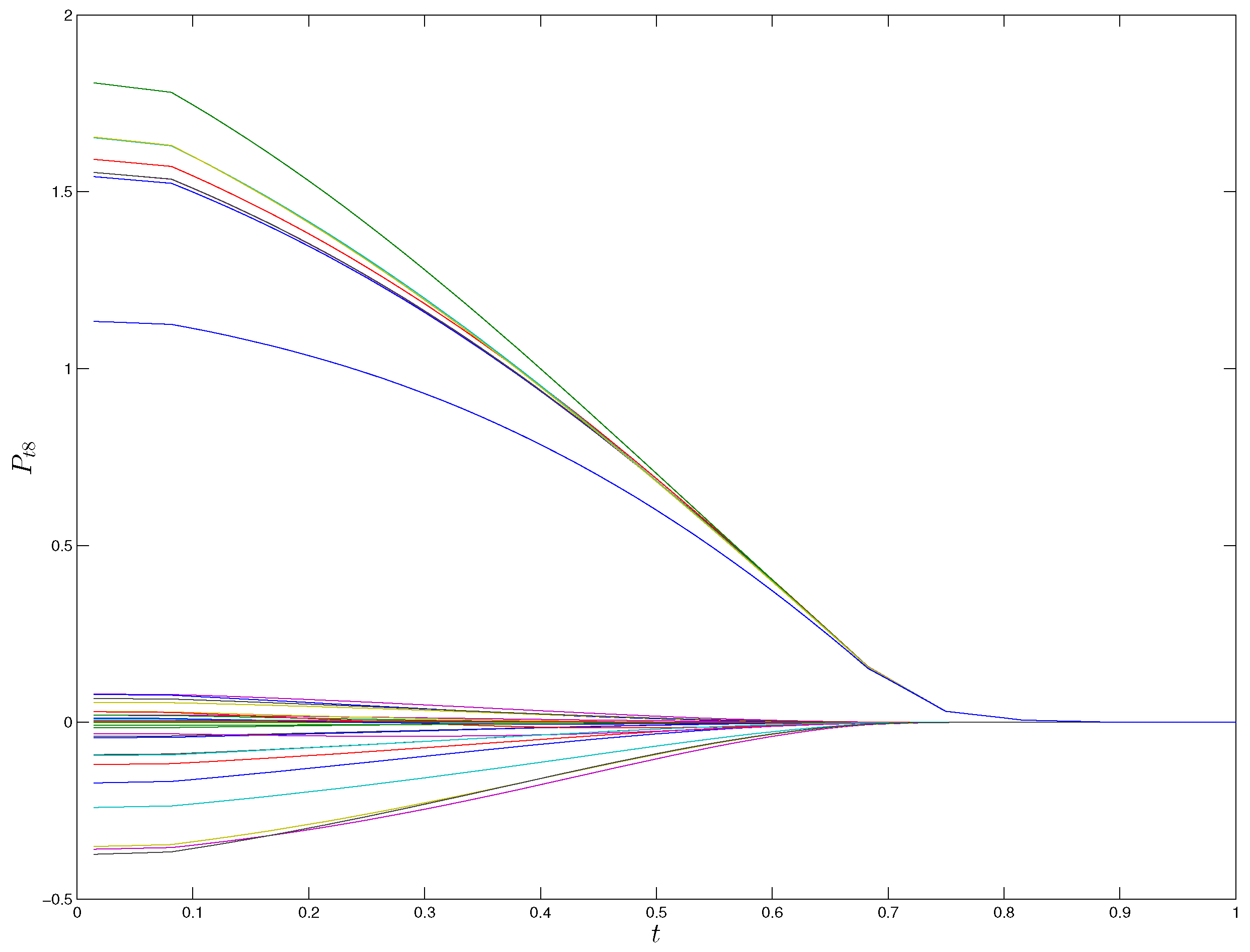
According to the 4th order explicit Runge–Kutta method, we obtain
by solving the Riccati Equation (
32). The plots of elements in
with respect to
t are shown in
Figure 1.
Substituting
into Equation (
34), we have the optimal control of problem (
30) by
By Equation (
35), the approximated optimal control of problem (
29) is
By Equation (
36), the inverse distribution
of
is
According to Equation (
37), the inverse distribution
of
is
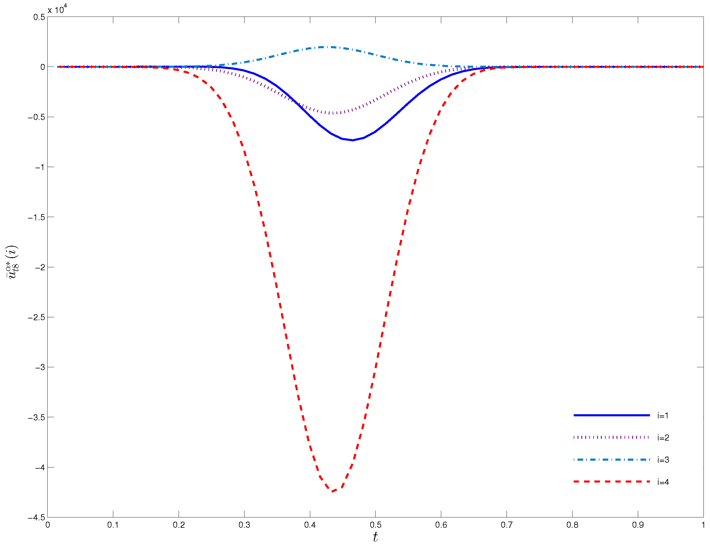
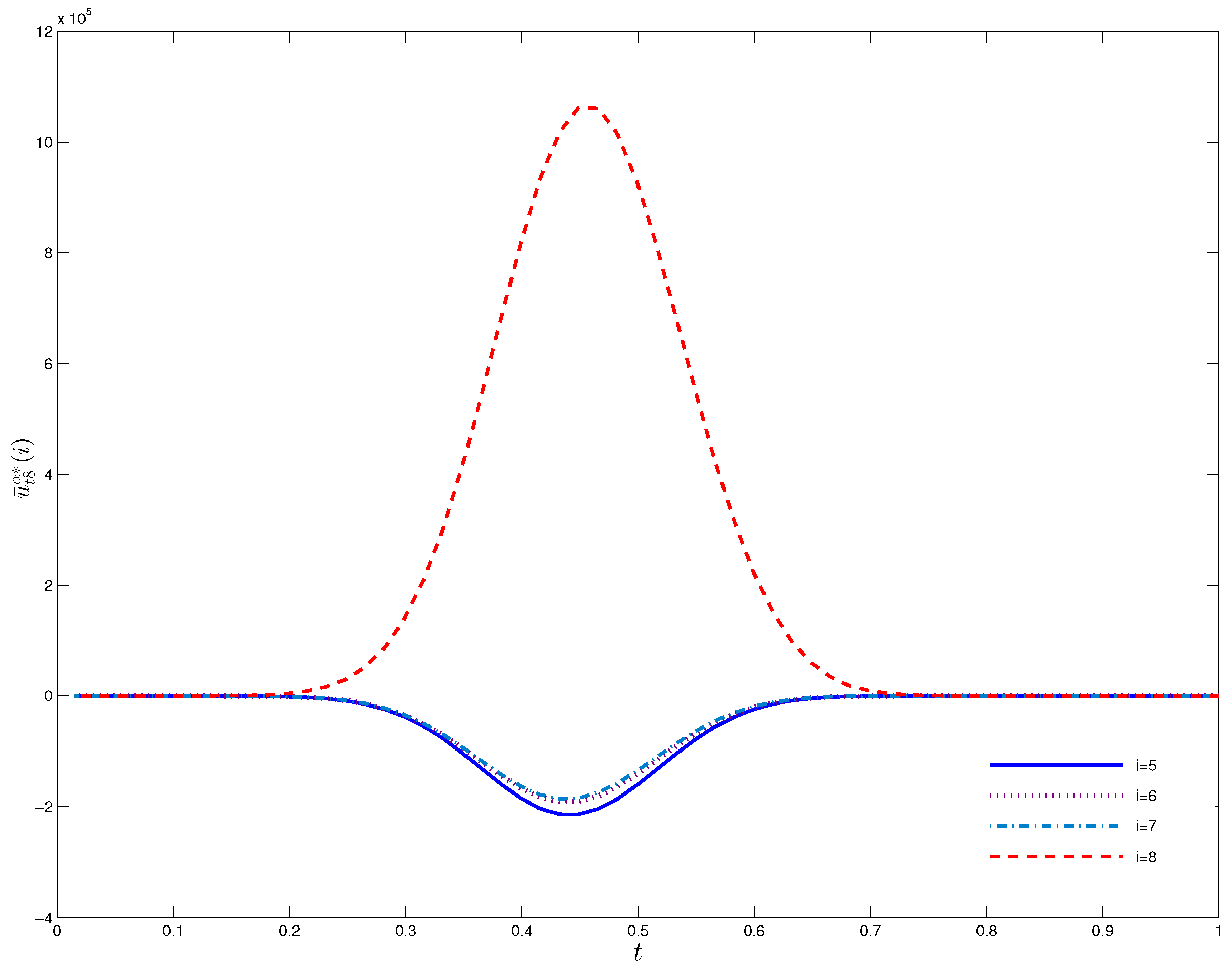
When
, elements of
with respect to
t are shown in
Figure 2 and
Figure 3. It can be seen from the figures that
and
have the most significant influence on
. Furthermore, the control directions of these two dimensions are opposite.
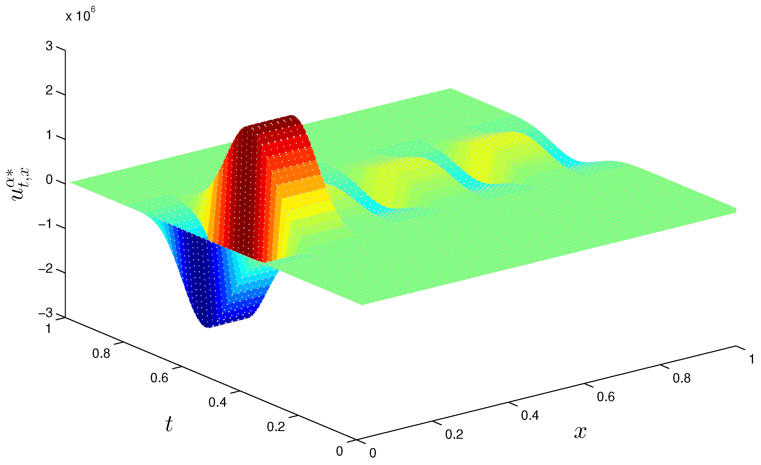
Figure 4 shows
with respect of
t and
x. For different positions,
x,
exhibits a positive and negative staggered form. The wavelet transform influences this form. As the wavelet basis dimension increases, the surface becomes smoother.
Substituting
to Equation (
33), we obtain the optimal value of problem (
30) is
. This suggests that the approximated optimal value of problem (
29) for
after wavelet transformation is
. In an environment with uncertain heat source, when we use an induction heater to keep the metal temperature stable, the approximated sum of the square of the temperature change of the metal itself and the temperature raised by the induction heater over time [0, 1] is at least
.


