RbfDeSolver: A Software Tool to Approximate Differential Equations Using Radial Basis Functions

Abstract

A new method for solving differential equations is presented in this work. The solution of the differential equations is done by adapting an artificial neural network, RBF, to the function under study. The adaptation of the parameters of the network is done with a hybrid genetic algorithm. In addition, this text presents in detail the software developed for the above method in ANSI C++. The user can code the underlying differential equation either in C++ or in Fortran format. The method was applied to a wide range of test functions of different types and the results are presented and analyzed in detail.

1. Introduction

A variety of problems in areas such as physics [1,2], chemistry [3,4,5], economics [6,7], biology [8,9], etc., can be modeled using ordinary differential equations (ODEs), systems of differential equations (SYSODEs) and partial differential equations (PDEs). Due to the importance of differential equations, several methods have appeared in the relevant literature, such as Runge–Kutta methods [10,11,12] or Predictor–Corrector methods [13,14]. Moreover, many methods based on machine learning models have appeared, such as methods that utilize neural networks [15,16,17], methods based on differential evolution techniques [18,19], genetic algorithms [20,21], etc. Furthermore, in recent years, a variety of methods that take advantage of modern GPU architectures have been published for the solution of differential equations [22,23,24]. In addition, a method based on Grammatical Evolution [25] has been introduced to solve differential equations in analytical form by Tsoulos and Lagaris [26], that creates solutions of differential equations in closed analytical form. Le et al. recently proposed [27] a Radial Basis Neural Network Approximation with extended precision for solving partial differential equations, and Wei et al. presented [28] a MATLAB code to solve differential equations with a conjunction of finite elements and Radial Basis Function network (RBF) neural networks. Additionally, a recent work based on quintic B-splines is proposed [29] for solving second-order coupled nonlinear Schrödinger equations. The current work proposes the incorporation of a modified genetic algorithm [30,31,32] and utilizes an RBF [33] to tackle the problem of solving differential equations. RBFs are usually expressed as:

$$r\left(x\right)=\sum _{i=1}^k{w}_i\varphi \left(∥x-c_i∥\right)$$

(1)

where the vector $\overrightarrow{x}$ is considered the input vector and the vector $\overrightarrow{w}$ is denoted as the weight vector. In many cases the function $\varphi \left(x\right)$ is a Gaussian function such as:

$$\varphi \left(x\right)=exp\left(-\frac{{\left(x-c\right)}^2}{{\sigma }^2}\right)$$

(2)

where the value $\varphi \left(x\right)$ depends on the distance between the vectors $\overrightarrow{x},$ $\overrightarrow{c}$. The vector x is considered the input to the artificial neural network and the vector c is called the centroid for the corresponding function. The centroid is often calculated from the input vectors using clustering techniques such as the KMeans [34] algorithm.

RBF networks have been used in many practical problems in various areas, such as physics [35,36,37,38], chemistry [39,40,41], medicine [42,43,44], economics [45,46,47], etc. In the current work, the RBF network is used as an estimator of the differential equations for the cases of ODEs, SYSODEs, and PDEs. The enforcement of the initial and boundary conditions is done through penalization. The parameters of the network are adapted through a hybrid genetic algorithm. The proposed study aims to present an innovative methodology for solving differential equations using RBF artificial neural networks, which are distinguished for their ability to learn and adapt to complex computational problems. However, in order to better adapt the parameters of these networks, their training is performed using an extremely reliable global optimization method, such as genetic algorithms. However, although network training with a genetic algorithms can achieve more accurate results, it is a rather time-consuming technique and is demanding of computational resources. This means that the use of modern parallel processing techniques is required, which will make the most of modern computing structures such as those of multiple cores. In the case of the proposed algorithm and the accompanying computing tool, the OpenMP programming library [48] was chosen.

In addition, the used software tool is illustrated in detail and some examples of usage are presented. The tool is designed for UNIX systems equipped with the GNU C++ and Fortran 77 (g77) compilers. Furthermore, the software utilizes the qmake installation utility of the QT software library, freely available from https://qt.io (accessed on 10 May 2022).

The rest of this article is organized as follows: in Section 2 the proposed method is fully described; in Section 3 the software details are presented; in Section 4 the experimental results for some differential equations are presented; and finally in Section 5 some conclusions and guidelines for future improvements of the method and the accompanied software are given.

2. Detailed Description

In the proposed method, an artificial RBF network with n weights is used as a function estimator that solves a differential equation. The initial and boundary conditions are imposed by the use of punitive factors. The network parameters are estimated using a hybrid genetic algorithm. The genetic algorithms are biologically inspired programming tools that maintain and evolve a pool of candidate solutions to an optimization problem. The members of this pool are usually called chromosomes or genetic population. The evolution of the population is done through the operations of mutation and crossover. Among other advantages, genetic algorithms are distinguished for their simplicity in implementation, for the ease of their parallelization, their tolerance for errors, etc. The size of each chromosome in the used genetic algorithm is calculated as: $d\times n+n+n$, where the value d is 1 for ODEs and system of ODEs and 2 for PDEs. The first $d\times n$ values are used for the centroid vectors $c_i$ of the Equation (1), the next n values are used for the $\sigma$ values of every Gaussian unit and the remaining n values of the chromosome are used for the weights $w_i$ of Equation (1). In addition, in the proposed implementation, a local optimization method is periodically applied to some randomly selected chromosomes of the population. This approach is performed in order to improve the accuracy of the solution produced by the genetic algorithm, but also to speed up the solution of the differential equation. The used local search procedure for this work was a BFGS variant of Powell [49].

In the following subsections, the proposed method is outlined in detail as well as the fitness calculation for every case of differential equation.

2.1. Main Algorithm

The steps of main the algorithm are described below:  

• Initialization step

  (a)

  Setiter = 0, as the current number of generations.

  (b)

  Set$N_c$, as the total number of chromosomes.

  (c)

  Setn, the number of weights in the RBF network.

  (d)

  Initialize randomly the chromosomes $X_i,i=1\dots N_c$.

  (e)

  Set ITERMAX as the maximum number of generations.

  (f)

  Set$p_s$ as the selection rate and $p_m$ the mutation rate.

  (g)

  Set$f_l=\infty$, the best fitness in the population.

  (h)

  Set $L_I$, the number of generations to run before applying the local optimization method

  (i)

  Set $L_c,$ the number of chromosomes that will involved in the local search procedure.

• Termination check. If$iter>$ ITERMAX OR $f_l\le ϵ$ terminate.
• Calculate the fitness $f_i$ for every chromosome $x_i$. The calculation procedure is described in Section 2.2.
• Genetic Operators

  (a)

  Selection procedure: During selection, the chromosomes are classified according to their suitability. The best $\left(1-p_s\right)\times N_c$ chromosomes are transferred without changes to the next generation of the population. The rest will be replaced by chromosomes that will be produced at the crossover.

  (b)

  Crossover procedure: During this process, $p_s\times N_c$ chromosomes will be created. Firstly, for every pair of produced offspring, two distinct chromosomes (parents) are selected from the current population using tournament selection: First, a subset of $K>1$ randomly selected chromosomes is created and the chromosome with the best fitness value is selected as parent. For every pair $(z,w)$ of parents, two new offsprings $\tilde{z}$ and $\tilde{w}$ are created through the following:

  $$\begin{array}{ccc}\hfill \widetilde{z_i}& =& a_i{z}_i+\left(1-a_i\right)w_i\hfill \\ \widetilde{w_i}& =& a_i{w}_i+\left(1-a_i\right)z_i\end{array}$$

  (3)

  where $a_i$ is a random number with the property $a_i\in [-0.5,1.5]$ [50].

  (c)

  Mutation procedure: For every element of each chromosome, select a random number $r\in \left[0,1\right]$ and alter the corresponding chromosome if $r\le p_m$.

• Setiter = iter+1
• Local Search Step

  (a)

  If$itersmod{L}_I=0$Then

  • Select a subset of $L_C$ randomly chosen chromosomes from the genetic population. Denote this subset with $L_S$.
  • For every chromosome $X_i$ in $L_S$
    • Start a local search procedure $y=L\left(x_i\right)$
    • Set$f_i=y$

  (b)

  Endif

• Denote with $f_l$ the best fitness value for the corresponding chromosome $x_l$
• Goto step 2.

2.2. Fitness Evaluation

The evaluation of the fitness is different for every case of differential equations, although in every case penalization is used to enforce the initial or the boundary conditions of every case.

2.3. Ode Case

Consider an ODE in the following format:

$$\psi \left(x,y,y^{\left(1\right)},\dots ,y^{\left(n\right)}\right)=0,x\in [a,b]$$

(4)

with $y^{\left(i\right)}$ the ith-order derivative of $y\left(x\right).$ The initial conditions are expressed as:

$$h_i{\left(x,y,y^{\left(1\right)},\dots ,y^{\left(n\right)}\right)}_{|x=t_i},i=1,\dots ,n$$

(5)

where $t_i$ could be a or b. The steps for the calculation of the fitness $f\left(g\right)$ of a chromosome g are the following for the ODE case:

• Create$T=\left\{x_1=a,x_2,x_3,\dots ,x_N=b\right\}$ a set of equidistant points.
• Create the RBF $r=r\left(g\right)$ network for the the chromosome g.
• Calculate the value $E_r={\sum }_{i=1}^N\psi {\left(x_i,r\left(x_i\right),r^{\left(1\right)}\left(x_i\right),\dots ,r^{\left(n\right)}\left(x_i\right)\right)}^2$
• Calculate the penalty value for the initial conditions:

  $$P_r=\lambda \sum _{k=1}^n{h}_k^2{\left(x,r\left(x\right),r^{\left(1\right)}\left(x\right),\dots ,r^{\left(n\right)}\left(x\right)\right)}_{|x=t_k}$$

  (6)

  where $\lambda >0$.
• Return$f\left(g\right)=E_r+P_r$

2.4. Systems of ODEs Case

The system of ODEs that should be solved is in the form:

$$\left(\begin{array}{ccc}{\psi }_1\left(x,y_1,y_1^{\left(1\right)},y_2,y_2^{\left(1\right)},\dots ,y_k,y_k^{\left(1\right)}\right)& =& 0\\ {\psi }_2\left(x,y_1,y_1^{\left(1\right)},y_2,y_2^{\left(1\right)},\dots ,y_k,y_k^{\left(1\right)}\right)& =& 0\\ ⋮& ⋮& ⋮\\ {\psi }_k\left(x,y_1,y_1^{\left(1\right)},y_2,y_2^{\left(1\right)},\dots ,y_k,y_k^{\left(1\right)}\right)& =& 0\end{array}\right)$$

(7)

with $x\in [a,b]$ and the initial conditions are expressed as:

$$\left(\begin{array}{ccc}{y}_1\left(a\right)& =& y_{1a}\\ y_2\left(a\right)& =& y_{2a}\\ ⋮& ⋮& ⋮\\ y_k\left(a\right)& =& y_{ka}\end{array}\right)$$

(8)

The fitness calculation $f\left(g\right)$ for a given chromosome g has as follows:

• Create$T=\left\{x_1=a,x_2,x_3,\dots ,x_N=b\right\}$ a set of equidistant points.
• Split the chromosome g into k parts and create the corresponding RBF networks $r_i=r\left(g_i\right)$
• Calculate the errors: $E_{r_i}={\sum }_{j=1}^N{\left({\psi }_i\left(x_j,r_1,r_1^{\left(1\right)},r_2,r_2^{\left(1\right)},\dots ,r_k,r_k^{\left(1\right)}\right)\right)}^2$
• Calculate the penalty values: $P_{r_i}=\lambda {\left(r_i\left(a\right)-y_{ia}\right)}^2$
• Calculate the total fitness value: $f\left(g\right)={\sum }_{i=1}^k\left(E_{r_i}+P_{r_i}\right)$

2.5. Pde Case

Consider a Pde in the following form:

$$h\left(x,y,\Psi (x,y),\frac{\partial }{\partial x}\Psi (x,y),\frac{\partial }{\partial y}\Psi (x,y),\frac{{\partial }^2}{\partial x^2}\Psi (x,y),\frac{{\partial }^2}{\partial y^2}\Psi (x,y)\right)=0$$

(9)

with $x\in [a,b],y\in [c,d]$. For Dirichlet boundary conditions we have the following condition functions:  

• $\Psi (a,y)=f_0\left(y\right)$
• $\Psi (b,y)=f_1\left(y\right)$
• $\Psi (x,c)=g_0\left(x\right)$
• $\Psi (x,d)=g_1\left(x\right)$

The steps to calculate the fitness $f\left(g\right)$ for any given chromosome are the following: 

• Construct the set $T=\left\{\left(x_1,y_1\right),\left(x_2,y_2\right),\dots ,\left(x_N,y_N\right)\right\}$ uniformly sampled points in $[a,b]\times [c,d]$.
• Construct the set $x_B=\left\{x_{b1},x_{b2},\dots ,x_{bM}\right\}$ equidistant points in $[a,b]$.
• Construct the set $y_B=\left\{y_{b1},y_{b2},\dots ,y_{bM}\right\}$ equidistant points in $[c,d]$.
• Set$r=r\left(g\right)$ the RBF network for the chromosome g.
• Calculate the quantity $E_r$ as

  $$E_r=\sum _{i=1}^{N}h{\left(x_i,y_i,r\left(x_i,y_i\right),\frac{\partial }{\partial x}r\left(x_i,y_i\right),\frac{\partial }{\partial y}r\left(x_i,y_i\right)\right)}^2$$
• Calculate the following penalty values:

  $$\begin{array}{ccc}{P}_{1r}& =& \lambda \sum _{i=1}^M{\left(r\left(a,y_{bi}\right)-f_0\left(y_{bi}\right)\right)}^2\\ P_{2r}& =& \lambda \sum _{i=1}^M{\left(r\left(b,y_{bi}\right)-f_1\left(y_{bi}\right)\right)}^2\\ P_{3r}& =& \lambda \sum _{i=1}^M{\left(r\left(x_{bi},c\right)-g_0\left(x_{bi}\right)\right)}^2\\ P_{4r}& =& \lambda \sum _{i=1}^M{\left(r\left(x_{bi},d\right)-g_1\left(x_{bi}\right)\right)}^2\end{array}$$
• Calculate the total fitness as $f\left(g\right)=E_r+P_{1r}+P_{2r}+P_{3r}+P_{4r}$

3. Software Details

3.1. Installation

The package is distributed in a zip file from the relevant GitHub URL https://github.com/itsoulos/RbfDeSolver (accessed on 10 May 2022) named RbfDeSolver-master.zip and under UNIX systems the user must execute the following commands to compile the software:

• unzip RbfDeSolver-master.zip.
• cd RbfDeSolver.
• qmake.
• make clean.
• make.

The final outcome of the compilation is the software RbfDeSolver. The differential equations should be compiled separately: every differential equation is a different file to be compiled as a shared object using the qmake utility. For example, in order to compile the ODE of the file ode1.so located under examples subdirectory, the user should create a ode1.pro file with the following contents:

 

TEMPLATE=lib

 

SOURCES=ode1.cc

Afterwards, the compilation of the ode is done using the following commands:

• qmake ode1.pro.
• make.

The outcome of the compilation is the shared library ode1.so

3.2. Command Line Options

The software RbfDeSolver has the following command line options:

• $--$help. Prints a help screen and terminates.
• $--$kind = DE_KIND. The string value DE_KIND determines the kind of differential equation to be used and the accepted values are: ode, sysode, pde.
• $--$problem = FILE, the string parameter file determines the path to the differential equation to be solved.
• $--$count = K, set as K, the number of chromosomes in the genetic population. The default value is 500.
• $--$random = R, set as R, the seed for the random number generation.
• $--$generations = G, set as G, the maximum number of generations allowed. The default value is 2000.
• $--$epsilon = E, set as E, a small positive value used in the comparisons as well as the termination criterion of the genetic algorithm. The default value is ${10}^{-7}$
• $--$weights = W, set as W, the number of weights for the RBF network. The default value is 1.
• $--$srate = S, set as S, the selection rate (parameter $p_s)$ of the genetic algorithm. The default value is 0.1
• $--$mrate = M, set as M, the mutation rate (parameter $p_m$) of the genetic algorithm. The default value is 0.05
• $--$lg = G, set as G, the number of generations that should be passed in the genetic algorithm before the local search method is applied. The default value is 100.
• $--$li = I, set as I, the number of chromosomes that will participate in the local search procedure. The default value is 20.
• $--$threads = T, set as T, the number of OpenMp threads. The default value is 1.

3.3. Format for ODEs

In Figure 1 and Figure 2 we present the formulation for ODEs in the languages C++ and Fortran correspondingly. The listed functions have the following meaning:  

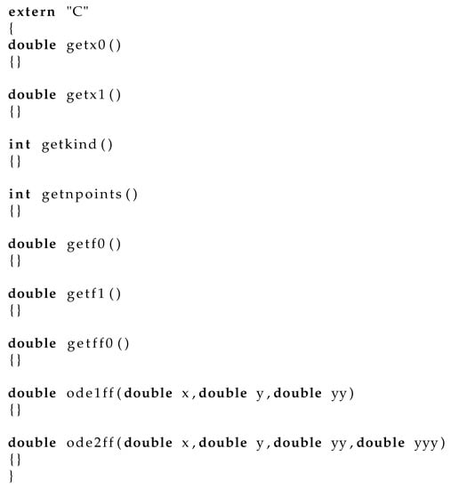
Figure 1. Ode format in C++.

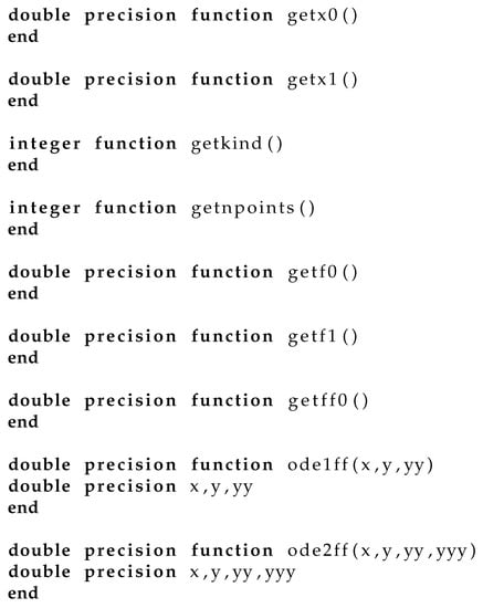
Figure 2. Ode format in Fortran.

• getx0(): Returns the lower boundary point, $x_0$.
• getx1(): Returns the upper boundary point, $x_1$.
• getkind(): Returns 1, 2 or 3:

  (a)

  If the value is 1 then the ODE is of first order and the boundary condition is of the form: $y\left(x_0\right)=y_0$.

  (b)

  If the value is 2 then the ODE is of second order with boundary conditions of the form: $y\left(x_0\right)=y_0,y^{\prime }\left(x_0\right)=y_0^{\prime }$.

  (c)

  Code 3 indicates that the ODE is of second order with boundary conditions of the form: $y\left(x_0\right)=y_0,y\left(x_1\right)=y_1$.

• getnpoints(): Returns the number of equidistant training points (value N in Section 2.3)
• getf0(): Returns the boundary condition on the left, $y_0$.
• getf1(): Returns the boundary condition on the right, $y_1$.
• getff0(): Returns the left boundary condition for second order ODEs $y_0^{\prime }$.
• ode1ff(x,y,yy): If the ODE is of first order, then the purpose of the tool is to minimize the function ode1ff$(x,r\left(x\right),r^{\left(1\right)}\left(x\right))$, for different values of x in the range $[x_0,x_1]$. The parameter y represents $r\left(x\right)$ and the parameter yy represents $r^{\left(1\right)}\left(x\right)$.
• ode2ff(x,y,yy,yyy): If the ODE is of second order, then the tool tries to minimize the function ode2ff$(x,r\left(x\right),r^{\left(1\right)}\left(x\right),r^{\left(2\right)}\left(x\right))$, for different values of x in the range $[x_0,x_1].$ The parameter y represents $r\left(x\right)$, the parameter yy represents $r^{\left(1\right)}\left(x\right)$ and the parameter yyy represents $r^{\left(2\right)}\left(x\right)$.

3.4. Format for System of ODEs

In Figure 3 and Figure 4 we demonstrate the formulation of System of ODES in C++ and in Fortran programming languages correspondingly. The functions used in those formulations have the following meanings:

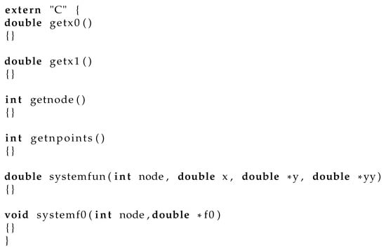
Figure 3. Format for SYSODEs in C++.

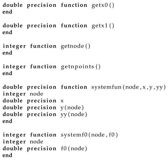
Figure 4. Format for SYSODEs in Fortran.

• getx0(): returns the left boundary, $x_0$.
• getx1(): returns the right boundary, $x_1$.
• getnode(): returns the number of ODEs in the system (parameter k in Section 2.4).
• getnpoints(): R returns the number of equidistant training points (value N in Section 2.4)
• systemfun(k,x,y,yy): For the SYSODE case, the aim of the RbfDeSolver is to minimize the function systemfun$(k,x,Y,Y^{\left(1\right)})$ for values of x in the range $[x_0,x_1]$, where k is the total number of equations in the system, Y is the vector of Rbf networks $r_i\left(x\right),i=1\dots k$ and $Y^{\prime }$ is a vector with elements the first derivative of these k equations evaluated at x. The double precision array y stands for the vector Y and similar the double precision array yy represents the vector $Y^{\prime }$.
• systemf0(node,f0): the argument node stands for the number of differential equations in the system and the double precision array f0 with node elements represents the vector holding the boundary conditions for each equation in the system (vector of Equation (8)).

3.5. PDE Format

The system is capable of solving elliptic PDEs in two dimensions in a box $[x_0,x_1]\times [y_0,y_1]$ with the Dirichlet boundary conditions $\Psi (x_0,y)=f_0\left(y\right)$, $\Psi (x_1,y)=f_1\left(y\right)$, $\Psi (x,y_0)=g_0\left(x\right)$ and $\Psi (x,y_1)=g_1\left(x\right)$. In Figure 5 and Figure 6 we can see the formulation of PDE’s in C++ and Fortran programming languages. The presented functions have the following representation:

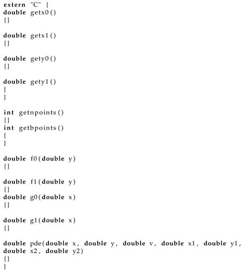
Figure 5. Format for PDEs in C++.

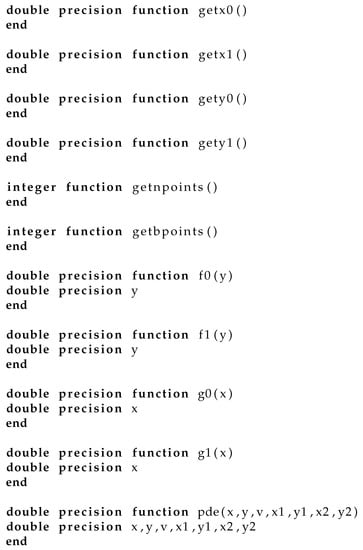
Figure 6. Format for PDEs in Fortran.

• getx0(): returns the left boundary $x_0$.
• getx1(): returns the right boundary $x_1$.
• gety0(): returns the left boundary $y_0$.
• gety1(): returns the right boundary $y_1$.
• getnpoints(): returns the amount of interior training points for the PDE.
• getbpoints(): returns the amount of training points across each boundary of the PDE.
• f0(y): returns the boundary condition $f_0\left(y\right)$ across $x=x_0$.
• f1(y): returns the boundary condition $f_1\left(y\right)$ across $x=x_1.$
• g0(x): returns the boundary condition $g_0\left(x\right)$ across $y=y_0$.
• g1(x): the function returns the boundary condition $g_1\left(x\right)$ across $y=y_1$.
• pde(x,y,v,x1,y1,x2,y2): For the PDE case RbfDeSolver minimizes the function $\mathrm{pde}\left(x,y,r(x,y),\frac{\partial r(x,y)}{\partial x},\frac{\partial r(x,y)}{\partial y},\frac{{\partial }^{2}r(x,y)}{\partial x^2},\frac{{\partial }^{2}r(x,y)}{\partial y^2}\right)$, where $x\in [x_0,x_1]$ and $y\in [y_0,y_1].$ The argument v corresponds to $r(x,y).$ The argument x1 corresponds to the first derivative of $r(x,y)$ with respect to x, y1 corresponds to the first derivative of $r(x,y)$ with respect to y, x2 corresponds to the second derivative of $r(x,y)$ with respect to x and the y2 corresponds to the second derivative of $r(x,y)$ with respect to y.

4. Experiments

A series of test functions used in various research papers [15,26] have been used here for testing purposes. All the problems have been coded in ANSI C++ and the execution was performed on a Intel i7-10700T running at 2.00 GHz with 16 GB of RAM, and the operating system was Debian Linux.

4.1. Linear ODEs

• ODE1

  $$y^{\prime }=\frac{2x-y}{x}$$

  with $y\left(1\right)=3,x\in [1,2]$. The solution is $y\left(x\right)=x+\frac{2}{x}$
• ODE2

  $$y^{\prime }=\frac{1-ycos\left(x\right)}{sin\left(x\right)}$$

  with $y\left(1\right)=\frac{3}{sin\left(1\right)},x\in [1,2]$. The solution is $y\left(x\right)=\frac{x+2}{sin\left(x\right)}$
• ODE3

  $$y^{″}=6y^{\prime }-9y$$

  with $y\left(0\right)=0,y^{\prime }\left(0\right)=2,x\in [0,1]$ and solution $y\left(x\right)=2xexp\left(3x\right)$
• ODE4

  $$y^{″}=-\frac{1}{5}{y}^{\prime }-y-\frac{1}{5}exp\left(-\frac{x}{5}\right)cos\left(x\right)$$

  with $y\left(0\right)=0,y\left(1\right)=\frac{sin\left(0.1\right)}{exp\left(0.2\right)},x\in [0,1]$ and solution $y\left(x\right)=exp\left(-\frac{x}{5}\right)sin\left(x\right)$
• ODE5

  $$y^{″}=-100y$$

  with $y\left(0\right)=0,y^{\prime }\left(0\right)=10,x\in [0,1]$ and the solution is

  $$y\left(x\right)=sin\left(10x\right)$$

4.2. Non-Linear ODEs

• LODE1

  $$y^{″}=\frac{1}{2y}$$

  with $y\left(1\right)=1,y\left(4\right)=2,x\in [1,4].$ The solution is $y\left(x\right)=\sqrt{x}$
• NLODE2

  $${\left(y^{\prime }\right)}^2+log\left(y\right)-{cos}^2\left(x\right)-2cos\left(x\right)-1-log(x+sin\left(x\right))=0$$

  with $y\left(1\right)=1+sin\left(1\right),x\in [1,2]$. The solution is $y\left(x\right)=x+sin\left(x\right)$
• NLODE3

  $$y^{″}{y}^{\prime }=-\frac{4}{x^3}$$

  with $y\left(1\right)=0,y\left(2\right)=log\left(4\right),x\in [1,2]$ and solution $y\left(x\right)=log\left(x^2\right)$
• NLODE4

  $$x^2{y}^{″}+{\left(x{y}^{\prime }\right)}^2+\frac{1}{log\left(x\right)}=0$$

  with $y\left(e\right)=0,y^{\prime }\left(e\right)=\frac{1}{e},x\in [e,2e]$ and solution $y\left(x\right)=log(log(x\left)\right)$

4.3. Systems of ODEs

• SYSODE1

  $$\begin{array}{ccc}\hfill y_1^{\prime }& =& cos\left(x\right)+y_1^2+y_2-\left(x^2+{sin}^2\left(x\right)\right)\hfill \\ \hfill y_2^{\prime }& =& 2x-x^{2}sin\left(x\right)+y_1{y}_2\hfill \end{array}$$

  with $y_1\left(0\right)=0,y_2\left(0\right)=0,x\in [0,1]$. The analytical solutions are $y_1\left(x\right)=sin\left(x\right)$, $y_2\left(x\right)=x^2$.
• SYSODE2

  $$\begin{array}{ccc}\hfill y_1^{\prime }& =& \frac{cos\left(x\right)-sin\left(x\right)}{y_2}\hfill \\ \hfill y_2^{\prime }& =& y_1{y}_2+exp\left(x\right)-sin\left(x\right)\hfill \end{array}$$

  with $y_1\left(0\right)=0,y_2\left(0\right)=1,x\in [0,1]$ and solutions $y_1\left(x\right)=\frac{sin\left(x\right)}{exp\left(x\right)},y_2=exp\left(x\right)$
• SYSODE3

  $$\begin{array}{ccc}\hfill y_1^{\prime }& =& cos\left(x\right)\hfill \\ \hfill y_2^{\prime }& =& -y_1\hfill \\ \hfill y_3^{\prime }& =& y_2\hfill \\ \hfill y_4^{\prime }& =& -y_3\hfill \\ \hfill y_5^{\prime }& =& y_4\hfill \end{array}$$

  with $y_1\left(0\right)=0,y_2\left(0\right)=1,y_3\left(0\right)=0,y_4\left(0\right)=1,y_5\left(0\right)=0,x\in [0,1]$ and solutions $y_1\left(x\right)=sin\left(x\right),y_2\left(x\right)=cos\left(x\right),y_3\left(x\right)=sin\left(x\right),y_4\left(x\right)=cos\left(x\right),y_5\left(x\right)=sin\left(x\right)$.
• SYSODE4

  $$\begin{array}{ccc}\hfill y_1^{\prime }& =& -\frac{1}{y_2}sin\left(exp\left(x\right)\right)\hfill \\ \hfill y_2^{\prime }& =& -y_2\hfill \end{array}$$

  with $y_1\left(0\right)=cos\left(1.0\right),y_2\left(0\right)=1.0,x\in [0,1]$ and solutions $y_1\left(x\right)=cos\left(exp\left(x\right)\right),$$y_2\left(x\right)=exp(-x)$.

4.4. PDEs

• PDE1

  $${\nabla }^2\Psi (x,y)=exp(-x)\left(x-2+y^3+6y\right)$$

  with $x\in [0,1],y\in [0,1]$ and boundary conditions: $\Psi (0,y)=y^3,\Psi (1,y)=\left(1+y^3\right)exp(-1),$$\Psi (x,0)=xexp(-x),\Psi (x,1)=(x+1)exp(-x)$ The solution is given by: $\Psi (x,y)=\left(x+y^3\right)exp(-x)$
• PDE2

  $${\nabla }^2\Psi (x,y)=-2\Psi (x,y)$$

  with $x\in [0,1],y\in [0,1]$ and boundary conditions: $\Psi (0,y)=0,\Psi (1,y)=sin\left(1\right)cos\left(y\right),$$\Psi (x,0)=sin\left(x\right),\Psi (x,1)=sin\left(x\right)cos\left(1\right)$. The analytical solution is $\Psi (x,y)=sin\left(x\right)cos\left(y\right)$.
• PDE3

  $${\nabla }^2\Psi (x,y)=4$$

  with $x\in [0,1],y\in [0,1]$ and boundary conditions: $\Psi (0,y)=y^2+y+1,\Psi (1,y)=y^2+y+3,$$\Psi (x,0)=x^2+x+1,\Psi (x,1)=x^2+x+3$. The solution is: $\Psi (x,y)=x^2+y^2+x+y+1$.
• PDE4

  $${\nabla }^2\Psi (x,y)=\left(x-2\right)exp(-x)+xexp(-y)$$

  with $x\in [0,1],y\in [0,1]$ and boundary conditions: $\Psi (0,y)=0,\Psi (1,y)=sin\left(y\right)$, $\Psi (x,0)=0,$$\Psi (x,1)=sin\left(x\right)$. The solution is: $\Psi (x,y)=sin\left(xy\right)$.

4.5. Experimental Results

To validate the ability of the proposed method to tackle differential equations, a series of experiments were made using the following values for the weight number of the Rbf network: $w=5,w=10,w=15$. The values for the parameters of the experiments are listed in Table 1. All the experiments were conducted 30 times using different seeds for the random number generator and the average error was measured. The random number generator used was the drand48() function of the C programming language. The experimental results are listed in Table 2.

Table 1. Experimental parameters.

Parameter	Value
$N_c$	1000
ITERMAX	5000
$p_s$	0.1
$p_m$	0.05
$ϵ$	${10}^{-7}$
$L_I$	100
$L_C$	20
$\lambda$	100

Table 2. Experimental results.

Equation	w = 5	w = 10	w = 15
ODE1	$3.9\times {10}^{-6}$	$2.2\times {10}^{-6}$	$3.4\times {10}^{-6}$
ODE2	$2.1\times {10}^{-5}$	$1.4\times {10}^{-5}$	$1.5\times {10}^{-5}$
ODE3	$6.6\times {10}^{-2}$	$7.7\times {10}^{-2}$	$9.4\times {10}^{-2}$
ODE4	$8.8\times {10}^{-7}$	$3.8\times {10}^{-6}$	$8.7\times {10}^{-7}$
ODE5	$9.4\times {10}^{-1}$	$1.1\times {10}^{-1}$	$5.9\times {10}^{-2}$
NLODE1	$7.2\times {10}^{-4}$	$1.6\times {10}^{-5}$	$1.9\times {10}^{-4}$
NLODE2	$4.6\times {10}^{-4}$	$5.3\times {10}^{-4}$	$1.1\times {10}^{-4}$
NLODE3	$5.7\times {10}^{-6}$	$7.9\times {10}^{-6}$	$5.4\times {10}^{-6}$
NLODE4	$1.2\times {10}^{-4}$	$7.9\times {10}^{-6}$	$2.6\times {10}^{-5}$
SYSODE1	$2.8\times {10}^{-6}$	$1.9\times {10}^{-6}$	$3.2\times {10}^{-6}$
SYSODE2	$1.4\times {10}^{-5}$	$3.2\times {10}^{-6}$	$3.9\times {10}^{-6}$
SYSODE3	$3.1\times {10}^{-5}$	$8.1\times {10}^{-5}$	$1.1\times {10}^{-5}$
SYSODE4	$1.4\times {10}^{-4}$	$4.4\times {10}^{-6}$	$6.4\times {10}^{-6}$
PDE1	$3.7\times {10}^{-2}$	$6.8\times {10}^{-3}$	$1.1\times {10}^{-2}$
PDE2	$3.2\times {10}^{-3}$	$2.1\times {10}^{-5}$	$2.2\times {10}^{-5}$
PDE3	$7.9\times {10}^{-2}$	$4.9\times {10}^{-4}$	$7.4\times {10}^{-4}$
PDE4	$8.0\times {10}^{-2}$	$7.8\times {10}^{-3}$	$3.4\times {10}^{-3}$

As the experimental results show, the proposed method solves the vast majority of differential equations even when the number of weights is relatively small. However, adding weights seems to have more positive effects on difficult problems especially in the case of partial differential equations. Of course, increasing the number of weights implies increased execution times and, for this reason, the use of parallel processing techniques is necessary. In the application, there is the possibility of using more processing threads through the OpenMP library.

In addition, the graphical representation of the produced solutions as well as the absolute error between the estimated RBF networks is also plotted. For example, in Figure 7 the solution of ODE1 and the estimated RBF network are plotted and in Figure 8 the absolute difference of these functions is plotted. Additionally, the absolute error between the solutions $y1\left(x\right)=sin\left(x\right),y\left(2\right)=x^2$ and the estimated RBF networks for the SYSODE1 case is also plotted in Figure 9. Moreover, the absolute error between the solution of the PDE1 case and the estimated RBF network is plotted in Figure 10. All graphs show the ability of the proposed method to approach to a large extent the solution of the differential equation which is under study.

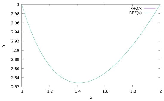
Figure 7. Graphical comparison between the solution of ODE1 and the estimated neural network.

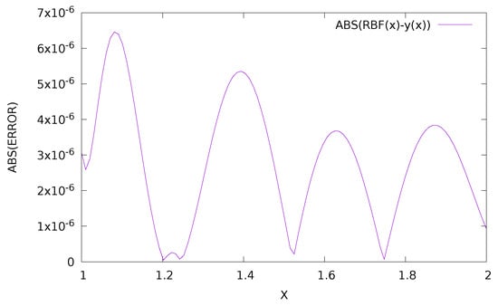
Figure 8. The absolute difference between the real solution of ODE1 and the produced RBF network.

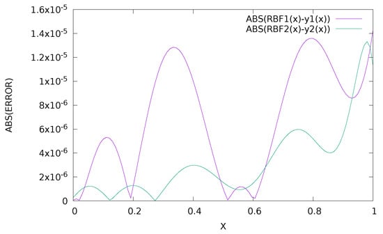
Figure 9. The difference between the functions $y1\left(x\right)=sin\left(x\right),y\left(2\right)=x^2$ and the estimated RBF solutions for the case of System of ODE’s SYSODE1.

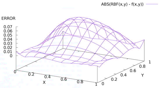
Figure 10. Absolute error between $f(x,y)=\left(x+y^3\right)exp(-x)$ and the estimated solution of PDE1.

Additionally, a plot was made to demonstrate the speed of the algorithm and the effectiveness of using more threads. In this test, the method was tested in ODE1 function for different values for the number of the threads and the desired accuracy (the value $-log10(ϵ$) for the parameter $ϵ$ in Table 2). The plot is shown in Figure 11. Execution times are significantly reduced as the number of threads increases and this makes the method able to be applied to more complex problems if there is enough computing power and several computing units available, which is possible in modern multi-core computers.

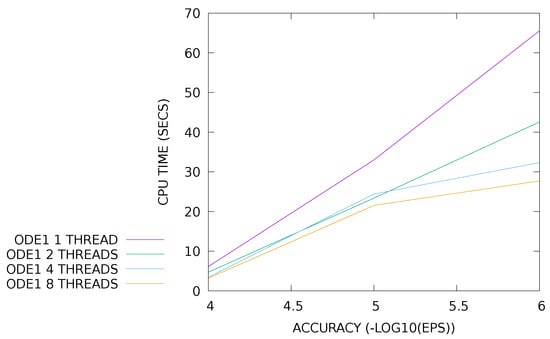
Figure 11. Computational cost and desired accuracy for different number of threads.

4.6. Some Practical Problems

The proposed method was also applied on a series of systems of ODEs available from https://archimede.uniba.it/testset/ (accessed on 10 May 2022) and more specific the Hires problem, the Rober problem, and the Orego problem.

4.6.1. Hires Problem

This is a system of eight non-linear ODEs proposed by Schäfer in 1975 [51] and it describes how light is involved in morphogenesis. The problem is defined as

$$\frac{dy}{dt}=f\left(y\right),y\left(0\right)=y_0$$

with $t\in [0,321.8122]$ and the function $f\left(y\right)$ defined as

$$\begin{array}{ccc}\hfill f\left(y\right)& =& \left(\begin{array}{c}-1.71y_1+0.43y_2+8.32y_3+0.0007\\ 1.71y_1-8.75y_2\\ -10.03y_3+0.43y_4+0.035y_5\\ 8.32y_2+1.71y_3-1.12y_4\\ -1.745y_5+0.43y_6+0.43y_7\\ -280y_6{y}_8+0.69y_4+1.71y_5-0.43y_6+0.69y_7\\ 280y_6{y}_8-1.81y_7\\ -280y_6{y}_8+1.81y_7\end{array}\right)\hfill \end{array}$$

and the initial conditions $y_0=\left(1,0,0,0,0,0,0,0.0057\right)$

4.6.2. Rober Problem

The Rober problem [52] describes the kinetics of an autocatalytic reaction and it is defined a system of three non-linear ordinary differential equations. The problem is defined as

$$\frac{dy}{dt}=f\left(y\right),y\left(0\right)=y_0$$

with $t\in [0,T]$ and the function $f\left(y\right)$ is

$$\begin{array}{ccc}\hfill f\left(y\right)& =& \left(\begin{array}{c}-0.04y_1+{10}^4{y}_2{y}_3\\ 0.04y_1-{10}^4{y}_2{y}_3-3\times {10}^7{y}_2^2\\ 3\times {10}^7{y}_2^2\end{array}\right)\hfill \end{array}$$

and the initial conditions $y_0=\left(1,0,0\right)$ and the value of T was set 10.

4.6.3. Orego Problem

The Orego problem [53] is a system of three non-linear ordinary differential equations and refers to the Oregonator model. The problem is defined as

$$\frac{dy}{dt}=f\left(y\right),y\left(0\right)=y_0$$

with $t\in [0,360]$ The function $f\left(y\right)$ is given by:

$$\begin{array}{ccc}\hfill f\left(y\right)& =& \left(\begin{array}{c}s\left(y_2-y_1{y}_2+y_1-q{y}_1^2\right)\\ \frac{1}{s}\left(-y_2-y_1{y}_2+y_3\right)\\ w\left(y_1-y_3\right)\end{array}\right)\hfill \end{array}$$

with $y_0=\left(1,2,3\right)$ and $s=77.27,w=0.161,q=8.375\times {10}^{-6}$.

The results from the application of the proposed method with the parameters of Table 1 and $w=10$ are listed in Table 3. The proposed method achieved low learning error even in the above examples. The column MEM denotes the application of the MEBDF [54] method to these problems. Furthermore, in Figure 12, Figure 13 and Figure 14, the average execution time of the proposed method for different number of processing threads is plotted for the previous three test cases. In these plots logarithmic scale was used.

Table 3. Experimental results for the real life problems.

Problem	w = 10	MEM
Hires	$2.8\times {10}^{-5}$	$6.1\times {10}^{-1}$
Rober	$2.1\times {10}^{-6}$	$1.2\times {10}^{-3}$
Orego	$2.7\times {10}^{-5}$	$2.5\times {10}^{-2}$

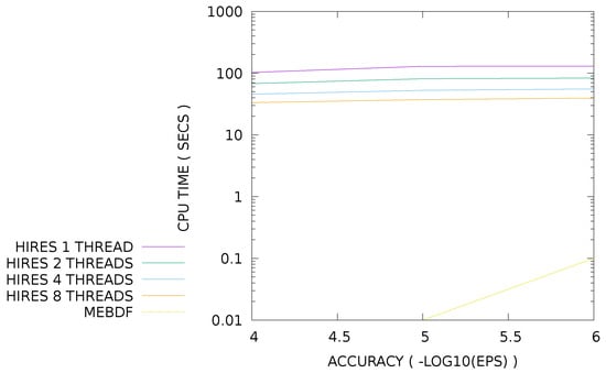
Figure 12. Computational cost and desired accuracy for different number of threads for the case of Hires problem.

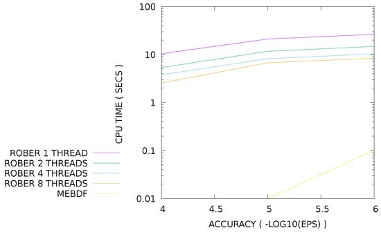
Figure 13. Computational cost and desired accuracy for different number of threads for the case of Rober problem.

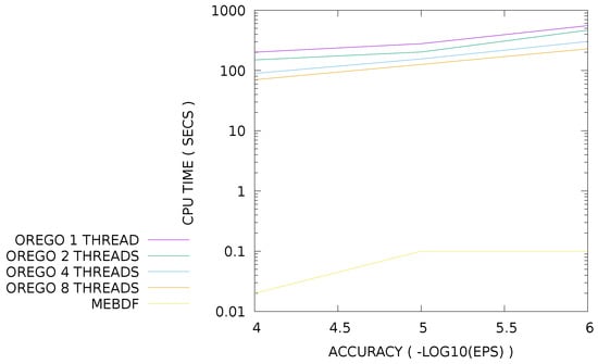
Figure 14. Computational cost and desired accuracy for different number of threads for the case of Orego problem.

5. Conclusions

A method for solving differential equations is presented here, accompanied by the corresponding software. The method utilizes gra networks to solve differential equations and the enforcement of initial and boundary conditions was done using penalty factors. The network configuration was adapted using a hybrid genetic algorithm, in which a local optimization method is applied to a randomly selected set of chromosomes per distinct number of generations.

The software developed in the context of this work was also presented. The software was written in C++ using the open source library QT, so that it can be run on most operating systems. The user can encode the differential equation in either C++ or Fortran by writing a series of functions. Future extensions of the method may include more efficient methods of initializing network weights as well as more advanced methods of terminating the genetic algorithm.

References

- Raissi, M.; Karniadakis, G.E. Hidden physics models: Machine learning of nonlinear partial differential equations. J. Comput. Phys. 2018, 357, 125–141. [Google Scholar] [CrossRef] [Green Version]
- Lelièvre, T.; Stoltz, G. Partial differential equations and stochastic methods in molecular dynamics. Acta Numer. 2016, 25, 681–880. [Google Scholar] [CrossRef]
- Scholz, G.; Scholz, F. First-order differential equations in chemistr. ChemTexts 2015, 1, 1. [Google Scholar] [CrossRef] [Green Version]
- Padgett, J.L.; Geldiyev, Y.; Gautam, S.; Peng, W.; Mechref, Y.; Ibraguimov, A. Object classification in analytical chemistry via data-driven discovery of partial differential equations. Comp. Math. Methods 2021, 3, e1164. [Google Scholar] [CrossRef]
- Owoyele, O.; Pal, P. ChemNODE: A neural ordinary differential equations framework for efficient chemical kinetic solvers. Energy 2022, 7, 100118. [Google Scholar] [CrossRef]
- Wang, Z.; Huang, X.; Shen, H. Control of an uncertain fractional order economic system via adaptive sliding mode. Neurocomputing 2012, 83, 83–88. [Google Scholar] [CrossRef]
- Achdou, Y.; Buera, F.J.; Lasry, J.M.; Lions, P.L.; Moll, B. Partial differential equation models in macroeconomics. Phil. Philos. Trans. R. Soc. A Math. Phys. Eng. Sci. 2012, 372, 20130397. [Google Scholar] [CrossRef] [Green Version]
- Hattaf, K.; Yousfi, N. Global stability for reaction—Diffusion equations in biology. Comput. Math. Appl. 2013, 66, 1488–1497. [Google Scholar]
- Getto, P.; Waurick, M. A differential equation with state-dependent delay from cell population biology. J. Differ. 2016, 260, 6176–6200. [Google Scholar] [CrossRef]
- Tang, W.; Sun, Y. Construction of Runge—Kutta type methods for solving ordinary differential equations. Appl. Math. Comput. 2014, 234, 179–191. [Google Scholar] [CrossRef]
- Kennedy, C.A.; Carpenter, M.H. Higher-order additive Runge–Kutta schemes for ordinary differential equations. Appl. Numer. Math. 2019, 136, 183–205. [Google Scholar] [CrossRef]
- Yang, X.; Shen, Y. Runge-Kutta Method for Solving Uncertain Differential Equations. J. Uncertain. Anal. Appl. 2015, 3, 17. [Google Scholar] [CrossRef] [Green Version]
- Kim, H.; Sakthivel, R. Numerical solution of hybrid fuzzy differential equations using improved predictor—Corrector method. Commun. Nonlinear Sci. Numer. Simul. 2012, 17, 3788–3794. [Google Scholar] [CrossRef]
- Daftardar-Gejji, V.; Sukale, Y.; Bhalekar, S. A new predictor–corrector method for fractional differential equations. Appl. Math. Comput. 2014, 244, 158–182. [Google Scholar] [CrossRef]
- Lagaris, I.E.; Likas, A.; Fotiadis, D.I. Artificial neural networks for solving ordinary and partial differential equations. IEEE Trans. Neural Netw. 1998, 9, 987–1000. [Google Scholar] [CrossRef] [PubMed] [Green Version]
- Mall, S.; Chakraverty, S. Application of Legendre Neural Network for solving ordinary differential equations. Appl. Soft Comput. 2016, 43, 347–356. [Google Scholar] [CrossRef]
- Pakdaman, M.; Ahmadian, A.; Effati, S.; Salahshour, S.; Baleanue, D. Solving differential equations of fractional order using an optimization technique based on training artificial neural network. Appl. Math. Comput. 2017, 293, 81–95. [Google Scholar] [CrossRef]
- Chang, W.D. Parameter identification of Chen and Lü systems: A differential evolution approach. Chaos Solitons Fractals 2007, 32, 1469–1476. [Google Scholar] [CrossRef]
- Biswas, A.; Das, S.; Abraham, A.; Dasgupta, S. Design of fractional-order PIλDμ controllers with an improved differential evolution. Eng. Appl. Artif. Intell. 2009, 22, 343–350. [Google Scholar] [CrossRef]
- Arqub, O.A.; Hammour, Z.A. Numerical solution of systems of second-order boundary value problems using continuous genetic algorithm. Inf. Sci. 2014, 279, 396–415. [Google Scholar] [CrossRef]
- Gutierrez-Navarro, D.; Lopez-Aguayo, S. Solving ordinary differential equations using genetic algorithms and the Taylor series matrix method. J. Phys. Commun. 2018, 2, 115010. [Google Scholar] [CrossRef] [Green Version]
- Januszewski, M.; Kostur, M. Accelerating numerical solution of stochastic differential equations with CUDA. Comput. Commun. 2010, 181, 183–188. [Google Scholar] [CrossRef] [Green Version]
- Murray, L. GPU Acceleration of Runge-Kutta Integrators. IEEE Trans. Parallel Distrib. Syst. 2012, 23, 94–101. [Google Scholar] [CrossRef]
- Riesinger, C.; Neckel, T.; Rupp, F. Solving Random Ordinary Differential Equations on GPU Clusters using Multiple Levels of Parallelism. Siam J. Sci. Comput. 2016, 38, C372–C402. [Google Scholar] [CrossRef]
- O’Neill, M.; Ryan, C. Grammatical evolution. IEEE Trans. Evol. Comput. 2001, 5, 349–358. [Google Scholar] [CrossRef] [Green Version]
- Tsoulos, I.G.; Lagaris, I.E. Solving differential equations with genetic programming. Genet. Program Evolvable Mach 2006, 7, 33–54. [Google Scholar] [CrossRef]
- Le, T.T.V.; Le-Cao, K.; Duc-Tran, H. A Radial Basis Neural Network Approximation with Extended Precision for Solving Partial Differential Equations. In Soft Computing: Biomedical and Related Applications. Studies in Computational Intelligence; Phuong, N.H., Kreinovich, V., Eds.; Springer: Berlin/Heidelberg, Germany, 2021; Volume 981. [Google Scholar]
- Wei, P.; Li, Z.; Li, X. An 88-line MATLAB code for the parameterized level set method based topology optimization using radial basis functions. Struct. Multidisc. Optim. 2018, 58, 831–849. [Google Scholar] [CrossRef]
- Iqbal, A.; Hamid, N.N.A.; Ismail, A.I.M.; Abbas, M. Galerkin approximation with quintic B-spline as basis and weight functions for solving second order coupled nonlinear Schrödinger equations. Math. Comput. Simul. 2021, 187, 1–16. [Google Scholar] [CrossRef]
- Goldberg, D. Genetic Algorithms in Search, Optimization and Machine Learning; Addison-Wesley Publishing Company: Boston, MA, USA, 1989. [Google Scholar]
- Michaelewicz, Z. Genetic Algorithms + Data Structures = Evolution Programs; Springer: Berlin/Heidelberg, Germany, 1996. [Google Scholar]
- Grady, S.A.; Hussaini, M.Y.; Abdullah, M.M. Placement of wind turbines using genetic algorithms. Renew. Energy 2005, 30, 259–270. [Google Scholar] [CrossRef]
- Park, J.; Sandberg, I.W. Universal Approximation Using Radial-Basis-Function Networks. Neural Comput. 1991, 3, 246–257. [Google Scholar] [CrossRef]
- MacQueen, J. Some methods for classification and analysis of multivariate observations. In Proceedings of the Fifth Berkeley Symposium on Mathematical Statistics and Probability, Los Angeles, CA, USA, 1 January 1967; Volume 1, pp. 281–297. [Google Scholar]
- Teng, P. Machine-learning quantum mechanics: Solving quantum mechanics problems using radial basis function networks. Phys. Rev. E 2018, 98, 033305. [Google Scholar] [CrossRef] [Green Version]
- Jovanović, R.; Sretenovic, A. Ensemble of radial basis neural networks with K-means clustering for heating energy consumption prediction. Fme Trans. 2017, 45, 51–57. [Google Scholar] [CrossRef] [Green Version]
- Alexandridis, A.; Chondrodima, E.; Efthimiou, E.; Papadakis, G.; Vallianatos, F.; Triantis, D. Large Earthquake Occurrence Estimation Based on Radial Basis Function Neural Networks. IEEE Trans. Geosci. Remote. Sens. 2014, 52, 5443–5453. [Google Scholar] [CrossRef]
- Gorbachenko, V.I.; Zhukov, M.V. Solving boundary value problems of mathematical physics using radial basis function networks. Comput. Math. Math. Phys. 2017, 57, 145–155. [Google Scholar] [CrossRef]
- Wan, C.; Harrington, P. Self-Configuring Radial Basis Function Neural Networks for Chemical Pattern Recognition. J. Chem. Inf. Comput. Sci. 1999, 39, 1049–1056. [Google Scholar] [CrossRef]
- Yao, X.; Zhang, X.; Zhang, R.; Liu, M.; Hu, Z.; Fan, B. Prediction of enthalpy of alkanes by the use of radial basis function neural networks. Comput. Chem. 2001, 25, 475–482. [Google Scholar] [CrossRef]
- Shahsavand, A.; Ahmadpour, A. Application of optimal RBF neural networks for optimization and characterization of porous materials. Comput. Chem. Eng. 2005, 29, 2134–2143. [Google Scholar] [CrossRef]
- Wang, Y.P.; Dang, J.W.; Li, Q.; Li, S. Multimodal medical image fusion using fuzzy radial basis function neural networks. In Proceedings of the 2007 International Conference on Wavelet Analysis and Pattern Recognition, Beijing, China, 2–4 November 2007; pp. 778–782. [Google Scholar]
- Mehrabi, S.; Maghsoudloo, M.; Arabalibeik, H.; Noormand, R.; Nozari, Y. Congestive heart failure, Chronic obstructive pulmonary disease, Clinical decision support system, Multilayer perceptron neural network and radial basis function neural network. Expert Syst. Appl. 2009, 36, 6956–6959. [Google Scholar] [CrossRef]
- Veezhinathan, M.; Ramakrishnan, S. Detection of Obstructive Respiratory Abnormality Using Flow—Volume Spirometry and Radial Basis Function Neural Networks. J. Med. Syst. 2007, 31, 461. [Google Scholar] [CrossRef]
- Momoh, J.A.; Reddy, S.S. Combined Economic and Emission Dispatch using Radial Basis Function. In Proceedings of the 2014 IEEE PES General Meeting|Conference & Exposition, National Harbor, MD, USA, 27–31 July 2014; pp. 1–5. [Google Scholar] [CrossRef]
- Guo, J.-J.; Luh, P.B. Selecting input factors for clusters of Gaussian radial basis function networks to improve market clearing price prediction. IEEE Trans. Power Syst. 2003, 18, 665–672. [Google Scholar]
- Falat, L.; Stanikova, Z.; Durisova, M.; Holkova, B.; Potkanova, T. Application of Neural Network Models in Modelling Economic Time Series with Non-constant Volatility. Procedia Econ. Financ. 2015, 34, 600–607. [Google Scholar] [CrossRef] [Green Version]
- Dagum, L.; Menon, R. OpenMP: An industry standard API for shared-memory programming. IEEE Comput. Sci. Eng. 1998, 5, 46–55. [Google Scholar] [CrossRef] [Green Version]
- Powell, M.J.D. A Tolerant Algorithm for Linearly Constrained Optimization Calculations. Math. Program. 1989, 45, 547. [Google Scholar] [CrossRef]
- Kaelo, P.; Ali, M.M. Integrated crossover rules in real coded genetic algorithms. Eur. J. Oper. 2007, 176, 60–76. [Google Scholar] [CrossRef]
- Schäfer, E. A new approach to explain the “high irradiance responses” of photomorphogenesis on the basis of phytochrome. J. Math. Biol. 1975, 2, 41–56. [Google Scholar] [CrossRef]
- Robertson, H.H. The Solution of a Set of Reaction Rate Equations. In Numerical Analysis: An introduction; Walsh, J., Ed.; Academic Press: Cambridge, MA, USA, 1967; pp. 178–182. [Google Scholar]
- Hairer, E.; Wanner, G. Solving Ordinary Di Erential Equations II: Sti and Di Erential-Algebraic PROBLEMS, 2nd revised ed.; Springer: Berlin/Heidelberg, Germany, 1996. [Google Scholar]
- Cash, R.; Considine, S. An MEBDF code for stiff initial value problems. Acm Trans. Math. Softw. 1992, 18, 142–158. [Google Scholar] [CrossRef]
Publisher’s Note: MDPI stays neutral with regard to jurisdictional claims in published maps and institutional affiliations. |
© 2022 by the authors. Licensee MDPI, Basel, Switzerland. This article is an open access article distributed under the terms and conditions of the Creative Commons Attribution (CC BY) license (https://creativecommons.org/licenses/by/4.0/).