Robust Spectral Clustering Incorporating Statistical Sub-Graph Affinity Model

Abstract

Hyperspectral image (HSI) clustering is a challenging work due to its high complexity. Subspace clustering has been proven to successfully excavate the intrinsic relationships between data points, while traditional subspace clustering methods ignore the inherent structural information between data points. This study uses graph convolutional subspace clustering (GCSC) for robust HSI clustering. The model remaps the self-expression of the data to non-Euclidean domains, which can generate a robust graph embedding dictionary. The EKGCSC model can achieve a globally optimal closed-form solution by using a subspace clustering model with the Frobenius norm and a Gaussian kernel function, making it easier to implement, train, and apply. However, the presence of noise can have a noteworthy negative impact on the segmentation performance. To diminish the impact of image noise, the concept of sub-graph affinity is introduced, where each node in the primary graph is modeled as a sub-graph describing the neighborhood around the node. A statistical sub-graph affinity matrix is then constructed based on the statistical relationships between sub-graphs of connected nodes in the primary graph, thus counteracting the uncertainty image noise by using more information. The model used in this work was named statistical sub-graph affinity kernel graph convolutional subspace clustering (SSAKGCSC). Experiment results on Salinas, Indian Pines, Pavia Center, and Pavia University data sets showed that the SSAKGCSC model can achieve improved segmentation performance and better noise resistance ability.

1. Introduction

Hyperspectral images (HSI) contain rich spectral and spatial information, which have been widely used in various fields, such as geological exploration, ocean monitoring, medical imaging, and forensics [1]. HSI classification, which aims to sort each pixel with a specific label, is the basis of HSI applications [2]. Supervised classification methods were the most commonly used for HSI classification [3,4]. In recent years deep learning models [5,6] and convolutional neural networks (CNNs) [7] have made significant progress in HSI classification. Due to the high cost of labeling training data, supervised classification methods are not available in HSI scenarios. Moreover, the supervised classification methods are challenging to handle unknown objects, since they are molded with existing classes.

To avoid the costs of manual data annotation, many works are devoted to expanding unsupervised HSI classification methods, i.e., HSI clustering. The HSI clustering is dedicated to seeking the intrinsic relationship between data points and determining labels in unsupervised rules automatically [8]. The critical point of HSI clustering is to measure the similarity between data points [9]. Traditional clustering methods often use Euclidean distance as a similarity measurement, such as K-means [10]. Due to unreliable measures, measures, mixed pixels, and the redundant banding problems [11], making the HSI clustering is extremely challenging [12]. Recently, subspace clustering [13] has become increasingly focused on HSI clustering [14] due to its ability to process high-dimensional data and its reliable performance. Technically, subspace clustering attempts to describe the data points as a linear combination of a self-expression dictionary in the same subspace [15]. The subspace clustering models typically include two parts, namely self-representation [16] and spectral clustering (SC) [17].

To expand the capability of subspace clustering, many works have been devoted to generating a robust affinity matrix. For example, sparse subspace clustering (SSC) [18] uses the $l_1$- norm to produce a sparse affinity matrix; low-rank subspace clustering (LRSC) [19] uses a nuclear norm to enforce the affinity matrix to be low-rank. By taking the spectral and spatial information into consideration, Zhang et al. proposed a spectral-spatial subspace clustering (S4C) [14]. By mapping the data into higher kernel spaces, kernel subspace clustering [20] became a nonlinear extension of the subspace clustering model. In [12], a modified kernel subspace clustering was utilized in HSI clustering.

The subspace clustering models based on Euclidean data often ignore the inherent graph structure information contained in HSI data points. HSI data points are easily affected by noise due to the interference of imaging spectrometers and the atmosphere [21]. Therefore, the traditional subspace model is sensitive to noisy images and abnormal data in the Euclidean domain. By transforming the HSI clustering into a clustering problem of non-Euclidean domain, the additional coefficients can be alleviated or even avoided by structural data.

The graph convolutional subspace clustering (GCSC) model [22] was used to recast the traditional subspace clustering into the non-Euclidean domain. By utilizing a graph convolutional self-representation model combining both graph and character information, the GCSC framework can circumvent noise data and tends to produce a more robust affinity than the traditional subspace clustering model.

For each pixel, a similarity matrix, or an affinity matrix, $W$ is constructed. In the matrix, $W_{uv}$ represents the degree of similarity between pixel $u$ and pixel $v$ [23]. The eigenvectors of the similarity matrix provide a measurement to identify the most significant features in the image. Ideally, each prominent image region is reformed into a set of data points in the eigenvector domain. Using clustering algorithms [24,25,26], such as k-means or hierarchically clustering [27], the resulting clusters are identified and labeled. As long as there are a sufficient number of sound measurements, spectral clustering can be valid for segmenting the image.

Two crucial challenges faced when applying spectral clustering are the noise-corrupted measurements and the texture variations within image regions [28]. In such situations, the pixels may be misclassified using traditional spectral clustering models, given their heavy reliance on the affinity between connected nodes to construct the affinity weighted graph; Pardo [29] extended pixel-to-pixel node affinity and proposed the idea of using region statistics to better classify the edges of regions in noisy images. Assuming that every region has a uniform intensity, for each part, the standard deviation and the mean are calculated. Areas with similar statistics are sorted into a single region, which does not consider the texture or region structure detected by the sub-graph method. Therefore, it is necessary to provide more robust image segmentation methods in the presence of heavy noise contamination.

The main contribution of this paper is the introduction of a robust spectral clustering method for image segmentation under heavy noise. Instead of relying on the node affinity between connected nodes, the proposed method utilizes the statistical sub-graph affinity between connected nodes to construct the affinity-weighted graphs [30]. By considering the spatial-intensity relationships within sub-graphs, it is assumed that the statistical affinity between sub-graphs is insensitive to noise, which is random and usually does not show such structural relations. By applying clustering graphs, which relate to the structure of objects, Luo [31] improves the robustness of spectral clustering. Instead, in the current work, the sub-graph was used to extend the affinity matrix including neighboring regions; the sub-graph affinity utilized region statistics before the clustering step so that similar regions, not similar nodes, will be clustered more robustly.

The rest of this article is structured as follows. We first briefly review the subspace clustering, graph convolutional subspace clustering, and HSI clustering in Section 2. Then, we present a detailed introduction of our proposed method in Section 3. In Section 4, the experimental data sets and experimental results are introduced. Finally, we conclude with a summary and future work in Section 5.

2. Related Work

2.1. Notations

Throughout this article, boldface lowercase italics symbols (e.g., $x$), boldface uppercase roman symbols (e.g., $X$), and regular italics symbols (e.g., $x_{ij}$) denote vectors, matrices, and scalars, respectively. A graph is represented as $G=(V,\epsilon ,A)$, where $V$ denotes the node set of the graph with $v_i\in V$ and $\left|V\right|=N$, $\epsilon$ indicates the edge set with $(v_i,v_i)\in \epsilon$, and $A\in R^{N\times N}$ stands for an adjacency matrix. We define the diagonal degree matrix of the graph as $D\in R^{N\times N}$, where $D_{ij}\in {\displaystyle {\sum }_j{A}_{ij}}$. The graph Laplacian is defined as $L=D-A$, and its normalized version is given by $L_{sym}=D^{-1/2}L{D}^{-1/2}$. In this article, $X^T$ denotes the transposition of matrix $X$ and $I_N$ denotes an identity matrix with the size of $N$. The Frobenius norm of a matrix is represented as ${\Vert X\Vert }_F={({\displaystyle {\sum }_{ij}|x_{ij}{|}^2})}^{1/2}$ and the trace of a matrix is defined as $tr(X)$.

2.2. Subspace Clustering Models

Let $X=[x_1,x_2,\dots ,x_N]\in R^{m\times N}$ be a collection of $N$ data points ${\{x_i\in R^m\}}_{i=1}^N$ and draw from a union of linear or affinity subspace $S_1\cup S_2\cup \dots \cup S_n$, where $N,m$ and $n$ denote the number of data points, features, and subspace, respectively. The subspace clustering model for the given data set is defined as the following self-representation problem [18]:

$$\min \left|\right|W|{|}_{p}s.t.XW=X,s.t.diag(W)=0$$

(1)

where $W\in R^{N\times N}$ denotes the self-expressive coefficient matrix and $diag(W)=0$ enforces the diagonal elements of $W$ to be zero so that the trivial solutions are avoided. $\left|\right|W|{|}_P$ denotes a $p-norm$ of matrix $W$, e.g., $\left|\right|W|{|}_1$(SSC) [18].

In the SSC model, the self-expressive coefficient matrix is conceived to be sparse so the self-representation problem is formulated as:

$$\arg \underset{W}{\min }\left|\right|XW-X|{|}_F^2+\lambda |\left|W\right|{|}_1,s.t.diag(W)=0$$

(2)

Here, the $l_1-norm$ tends to cause a sparse coefficient matrix. By using a nuclear norm, LRSC [19] rewrites the self-expression problem as:

$$\arg \underset{W}{\min }\left|\right|XW-X|{|}_{2,1}^2+\lambda |\left|W\right|{|}_{\ast },s.t.diag(W)=0$$

(3)

where $\left|\right|\cdot |{|}_{\ast }$ and $\left|\right|\cdot |{|}_{2,1}$ denote the nuclear norm and $l_{2,1}-norm$ of a matrix. LRSC has been proven to incorporate the structure of data effectively. The above problem can be solved by using the alternating direction method of multipliers (ADMM [32]). Once the coefficient matrix $W$ is found, the subspace clustering pursues the partition of affinity matrix $A=(1/2)(|W|+|W{|}^T)$ using the SC method [24].

2.3. GCSC Framework

By incorporating graph embedding into subspace clustering, we refer to the framework as GCSC. The aim of the GCSC framework is to use graph convolution to learn a robust affinity. For this target, we modify the traditional self-representation as follows:

$$X=X\overline{A}Z,s.t.diag(Z)=0.$$

(4)

Here, $Z\in R^{N\times N}$ is the self-representing coefficient matrix and $\overline{A}={\tilde{D}}^{-1/2}\tilde{A}{\tilde{D}}^{-1/2}$ denotes the normalized adjacency matrix with self-loops [28]. The $X\overline{A}Z$ operation will preserve the structure and inherent attributes of the graph by embedding the graph into vector space. We call (4) a graph convolutional self-representation. Similar to the traditional subspace clustering model, the GCSC framework can be rewritten as:

$$\arg \underset{Z}{\min }\frac{1}{2}\left|\right|X\overline{A}Z-X|{|}_q+\frac{\lambda }{2}|\left|Z\right|{|}_p,s.t.diag(Z)=0$$

(5)

where $q$ and $p$ denote any suitable matrix norm, such as $p,q=0,(1/2),1,2$ and nuclear norm, and $\lambda$ is a trade-off coefficient. It is easy to prove that the traditional subspace models are a special case of this framework, i.e., the traditional subspace clustering models depend only on data features. For example, when the Frobenius norm and $p=1$ (5) becomes an extension of the classical SSC [18], while $q$ is $l_{2,1}-norm$ and $p$ is nuclear norm, (5) degenerates to LRSC [19]. Equation (5) can be efficiently solved by the same methods adopted in traditional subspace clustering methods. Once the self-represented coefficient matrix is obtained, the spectral clustering (SC) can be used to generate clustering results.

2.4. HSI Clustering Using the GCSC Models

Two essential matters need to be solved before we use the GCSC model. First, HSI data usually contain many spectral bands with redundancy, so it is difficult to obtain acceptable performance using only spectral features. Second, the HSI uses Euclidean data, whereas GCSC models are based on graph-structured data [29].

To solve the first problem, we use principal component analysis (PCA) to reduce the spectral dimension by retaining the top $d$ PCs [30]. This not only reduces the redundant information contained in the HSI data but also improves the computational efficiency during model training. To take spectral and spatial information into consideration, we represent each data point by extracting three-dimensional data blocks [31]. Specifically, every data point is represented by the central and neighboring pixels. This method has been widely used in different HSI spectral-spatial classification models [32]. For the second problem, a k-nearest neighbor (k-NN) graph was constructed to substitute the graph structure of the data points. Specifically, each data point is viewed as a node in the graph, and the k-NNs of $x_i$ consist of edge relations. The adjacency matrix $A$ of a k-NN graph is defined as:

$$A_{ij}=\{\begin{array}{l}1,x_j\in N_k(x_i)\\ 0,otherwise\end{array}$$

(6)

where $N_k(x_i)$ indicates the k-NNs of $x_i$, which is determined by computing the pairwise Euclidean distance between the PCA reduced data points.

3. Methodology

SSAKGCSC

Based on the GCSC framework, statistical sub-graph affinity model, and Gaussian kernel function mentioned above, the statistical sub-graph affinity kernel GCSC (SSAKGCSC) is proposed. In this section, we introduce the establishment and the derivation process of the SSAKGCSC model.

We set both $q$ and $p$ to be the Frobenius norm in the GCSC model. Formally, we denote it as:

$$\arg \underset{Z}{\min }\frac{1}{2}\left|\right|X\overline{A}Z-X|{|}_F^2+\frac{\lambda }{2}|\left|Z\right|{|}_F^2.$$

(7)

Ji et al. [33] has proven that the Frobenius norm will not obtain trivial results even without the constraint $diag(Z)=0$. Solving the above equation leads to a dense matrix of self-representing coefficients and a valid closed-form solution. We can rewrite (7) as:

$$\begin{array}{cc}\hfill L\left(Z\right)& =\frac{1}{2}\left|\right|X\overline{A}Z-X|{|}_F^2+\frac{\lambda }{2}{\Vert Z\Vert }_F^2\hfill \\ & =\frac{1}{2}tr[{(X\overline{A}Z-X)}^T(X\overline{A}Z-X)+\lambda Z^{T}Z]\hfill \\ & =\frac{1}{2}tr(Z^T{\overline{A}}^T{X}^{T}X\overline{A}Z+X^{T}X-2X^{T}X\overline{A}Z+\lambda Z^{T}Z)\hfill \end{array}$$

(8)

According to matrix trace and matrix derivative, the partial derivative of $L$ for $Z$ can be expressed as:

$$\begin{array}{cc}\hfill \frac{\partial L}{\partial Z}& ={\overline{A}}^T{X}^{T}X\overline{A}Z-{\overline{A}}^T{X}^{T}X+\lambda Z\hfill \\ & =({\overline{A}}^T{X}^{T}X\overline{A}+\lambda I_N)Z-{\overline{A}}^T{X}^{T}X.\hfill \end{array}$$

(9)

Let $\frac{\partial L}{\partial Z}=0$; we get:

$$({\overline{A}}^T{X}^{T}X\overline{A}+\lambda I_N)Z={\overline{A}}^T{X}^{T}X.$$

(10)

Finally, matrix $Z$ can be expressed as:

$$Z={({\overline{A}}^T{X}^{T}X\overline{A}+\lambda I_N)}^{-1}{\overline{A}}^T{X}^{T}X.$$

(11)

Due to ${\overline{A}}^T{X}^{T}X\overline{A}+\lambda I_N$ being positive semi-definite, its inverse matrix always exist.

Unlike traditional subspace clustering models that usually require iterative optimization, this algorithm ensures high computational efficiency. Once matrix $Z$ is obtained, we can use it to build an affinity matrix for spectral clustering. Most works compute the affinity matrix by $C=|Z{|}^T+|Z|$ or $\left|Z\right|$ [34]. In this work, we use the heuristic method employed by efficient dense subspace clustering (EDSC) [35] to enhance the block structure, which has been shown to benefit the accuracy of clustering.

Due to the complexity and nonlinearity of HSI, a large body of works has demonstrated that nonlinear models will achieve better performance than their linear counterparts [36]. Therefore, we use the kernel trick for its nonlinear extension.

Let $\varphi :R^m\to H$ be a mapping from the input space to the regeneration kernel Hilbert space $H$; we define a positive semi-definite kernel Gram matrix $K_{XX}\in R^{N\times N}$ as:

$${[K_{XX}]}_{ij}=[{⟨\varphi (X),\varphi (X)⟩}_H]=\varphi {(x_i)}^T\varphi (x_j)$$

(12)

where $k:R^m\times R^m\to R$ denotes the kernel function. The Gaussian kernel has been widely used in other subspace clustering models, i.e., $k(x_i,x_j)=\exp (-\gamma ||x_i-x_j|{|}^2),$ where $\gamma$ is the parameter of the Gaussian kernel function [37]. Then the EKGCSC model can be expressed as:

$$\arg \underset{Z}{\min }\frac{1}{2}\left|\right|\varphi (X)\overline{A}Z-\varphi (X)|{|}_F^2+\frac{\lambda }{2}|\left|Z\right|{|}_F^2.$$

(13)

By using the kernel trick, (13) can be rewritten as:

$$\arg \underset{Z}{\min }\frac{1}{2}tr(Z^T{\overline{A}}^T{K}_{XX}\overline{A}Z-2K_{XX}\overline{A}Z+K_{XX}+\lambda Z^{T}Z).$$

(14)

The above equation can be solved by taking the partial derivative of $Z$ and setting the result to zero, so (14) can be reformulated as:

$$L\left(Z\right)=\frac{1}{2}tr(Z^T{\overline{A}}^T{K}_{XX}\overline{A}Z-2K_{XX}\overline{A}Z+K_{XX}+\lambda Z^{T}Z).$$

(15)

The partial derivative of L for Z can be expressed as:

$$\begin{array}{cc}\hfill \frac{\partial L}{\partial Z}& ={\overline{A}}^T{K}_{XX}\overline{A}Z-{\overline{A}}^T{K}_{XX}+\lambda Z\hfill \\ & =({\overline{A}}^T{K}_{XX}\overline{A}Z+\lambda I_N)Z-{\overline{A}}^T{K}_{XX}.\hfill \end{array}$$

(16)

Let $\frac{\partial L}{\partial Z}=0$; we obtain the closed form solution as:

$$Z={({\overline{A}}^T{K}_{XX}\overline{A}+\lambda I_N)}^{-1}{\overline{A}}^T{K}_{XX}.$$

(17)

This model maps the data points onto a higher-dimensional space, thus making a linearly inseparable issue a detachable one.

The model improves the robustness of spectral clustering by replacing the node affinity $K_{XX}$ used in (17) with the concept of statistical sub-graph affinity.

$$W_{uv}=\exp \{-\frac{(x_u-x_v)}{2{\sigma }^2}\}$$

(18)

To create an affinity matrix, the connectivity of each node must be expressed by a connectivity graph $G$. $G$ is implicitly constructed from graph kernels $K$. The kernel weights, elements of $K$, manifest the connectivity between a node and its neighbor. The method introduces a statistical sub-graph affinity model to substitute the node affinity model [38]. Instead of comparing $x_u$ to $x_v$ for $v$ in the neighbor of $u$, the sub-graph $P_u$ is compared against each sub-graph $P_v$, which is illustrated in Figure 1.

Figure 1. Comparison of node affinity to sub-graph affinity. $x_u$ (red), $x_v$ (green), $P_u$ (light red), $P_v$ (light green). (a) Node affinity. (b) Node affinity with neighborhood statistics. (c) Sub-graph affinity.

A mathematical description is used to understand how sub-graphs can improve classification accuracy. Assuming the node $u$ belonging to a class $C_k$, the node features, $x_u$ can be regarded as the random processes, $X_u$, subject to independent identical distribution (i.i.d.) noise, $N$:

$$X_u={\mu }_u+N,$$

(19)

where ${\mu }_u$ is the mean of all node features belonging to class $C_k$.

The sub-graph contains the connectivity of node $u$ to its neighbors. When using node affinity, the probability that two nodes, $u$ and $v$, belong to the same class, $P(u\in C_k\mathrm{and}v\in C_k)$, denoted as $P_{u,v,node}$, is the probability that the difference between $X_u$ and $X_v$ is equal to zero:

$$P_{u,v,node}=P(X_u-X_v=0|C_k).$$

(20)

Since $X_u$ and $X_v$ are i.i.d., then $P_{u,v,node}$ can be confirmed using the Laplace distribution [39]:

$$P_{u,v,node}=\frac{1}{{(2b)}^n}\exp (-\frac{|x_u-x_v|}{b})$$

(21)

where $b$ is a coefficient related to $N$. The sub-graph affinity restrains the noise compared to the node affinity. The obtained sub-graph affinity probability $P_{sub}$ is equal to:

$$P_{u,v,sub}={\displaystyle \prod _{i}P(X_{u,i}-X_{v,i}=0|C_k)}.$$

(22)

$$P_{u,v,sub}={\displaystyle \prod _i\frac{1}{{(2b)}^n}\exp (-\frac{|x_{u,i}-x_{v,i}|}{b})}$$

(23)

where $i$ is the index of each factor in $P_u$ and the corresponding element in $P_v$. The more similar the distribution in each sub-graph, the smaller $x_{u,i}-x_{v,i}$ becomes, and the larger the probability of $P(u\in C_k\mathrm{and}v\in C_k)$. So, the local neighborhood information can help suppress the noise.

Given the proposed statistical sub-graph affinity model, we incorporated this model into the spectral clustering framework by introducing a weighting matrix into (17) [40]. The density of $W$ mainly depends on the complexity of $G$ and is independent of $P_u.$ The value of $W$, which depends on the kernel weights and the statistical sub-graph affinity, can be defined as:

$$w_{uv}=K_{u-v}{\displaystyle \prod _i\exp \{-\frac{{((x_{u+i}-x_{v+i})\cdot P_{u,i})}^2}{2{\sigma }^2}\}}$$

(24)

For node $u$ and node $v$, The weights related with $K_u$ and $P_u$ are also imported to allow spatial weighting.

The following shows how $K_u$ and $P_u$ influence the size of the neighborhood and the computational complexity of (23). Increasing the size of $K$ increases the size of the neighborhood; therefore, the number of $x_u$ and $x_v$ increases, which leads to decreasing the sparsity of $W$. Increasing the size of $P_u$ does not affect the neighborhood size and, consequently, it does not affect the sparsity of $W$. The increased size of $P_u$ only increases the computational complexity of calculating $w_{uv}$ moderately. The difference of $x_u$ and $x_v$ can be saved after first calculation. Hence, the size of $K$ makes a more noteworthy effect on the overall computational complexity than the size of $P_u$.

By choosing a radially symmetric kernel, the algorithm can be rotationally invariant. The kernel can also empower distance information so that the weights or connectivity of the sub-graph can be a function of spatial distance, i.e., the intensity difference of the relevant pixel can be weighted according to the distance from the center of the sub-graph [41]. By integrating the spatial intensity relationships within the sub-graph into the construction of the affinity weighted graph, the constructed graph is less sensitive to random noise. Consequently, the statistical sub-graph affinity model is stronger against noise.

We use (24) as a newly introduced ‘Gaussian kernel’ to implement the combination of the sub-graph affinity model with the GCSC model, which we denote as K0; the result of multiplying (24) with the Gaussian kernel is denoted as K0 × K1.

4. Experiments Results

4.1. Setup

4.1.1. Data Sets and Preprocessing

We implemented experiments on four HSI data sets: Salinas, Indian Pines corrected, Pavia Center, and Pavia University. For computational efficiency, we take a sub-scene of each of these data sets for evaluation [35,36], Specifically, these sub-scenes are located at [591–676, 158–240], [30–115, 24–94], [100–250, 200–350], and [150–350, 100–200], respectively. The sub-scenes obtained from the Salinas data set is referred to as the SalinasA data set. The detailed information of these four data sets were demonstrated in Table 1. In the data preprocessing phase, we reduced the spectral bands into four by retaining at least 96% of the cumulative percent variance (CPV) by PCA [42]. We constructed the spectral-spatial blocks by setting the neighborhood size to be nine for data sets. All data points were normalized by scaling into [0, 1] before clustering.

Table 1. Summary of SalinasA, Indian Pines, Pavia University, and Pavia Center data sets.

Data Sets	SalinasA	Indian Pines Corrected	Pavia University	Pavia Center
Pixels	83 × 86	85 × 70	140 × 150	150 × 150
Channels	204	200	103	103
Clusters	6	4	8	7
Samples	5348	4391	6445	5710
Sensor	AVIRIS	AVIRIS	ROSIS	ROSIS

Since the HSI image with considerable noise cannot be obtained, we decided to add noise into these images manually. In the process of adding noise to HSI images, we noticed that, due to the unique characteristics of HSI images, the maximum value in each channel was no longer 255 as in RGB images, but varied from dozens to 8000. If all dimensions of a hyperspectral image are normalized uniformly, it is easy to produce smaller numbers and affect the algorithm’s stability. For these reasons, each dimension of the HSI image was normalized separately, and then Gaussian noise and salt and pepper noise was added to it.

4.1.2. Evaluation Metrics

Three noted metrics [12,25,35], are used to estimate the clustering performance of the clustering model, i.e., overall accuracy (OA), normalized mutual information (NMI), and Kappa coefficient (Kappa). These metrics range from 0 to 1, where the larger the value are, the more exact the clustering results are obtained. To assess the computational complexity of the models, we compared the running time of different models in our experiments.

4.1.3. Compared Methods

We compared the SSAKGCSC method with some HSI clustering methods, including traditional clustering methods and superior methods. To be specific, the traditional clustering methods include sparse subspace clustering (SSC) [6], efficient dense subspace clustering (EDSC) [24], and low-rank subspace clustering (LRSC) [27]. The relatively superior HSI clustering methods are spectral-spatial subspace clustering (S4C) [15], efficient graph convolutional subspace clustering (EGCSC) [31], and efficient kernel graph convolutional subspace clustering (EKGCSC) [31].

We follow their settings published in the corresponding paper for the HSI clustering methods mentioned above. The hyperparameters of SSAKGCSC are given in Table 2. All the compared methods are implemented with Python 3.7 running on an Intel(R) Core (TM) i5-5200U CPU @ 2.20GHz CPU with 8GB RAM.

Table 2. Settings of the important hyperparameters in SSAKGCSC.

Data Sets	Noise	REG_Coef	GAMMA	NEIGHBOR	RO	post_proC	Kernel
	- 1	100	0.2
SalinasA.	+sp 2	0.01	0.2	30	0.8	8, 18	K0
	+gs 3	100	0.2
	+sg 4	1	0.2
	- 1	10,000	10
Indian Pines.	+sp 2	100,000	0.1	30	0.8	17, 15	K0 × K1
	+gs 3	100,000	0.01
	+sg 4	1,000,000	0.001
	- 1	60,000	65
Pavia University	+sp 2	150	100	30	0.8	8, 18	K0 × K1
	+gs 3	10	100
	+sg 4	500	100
	- 1	0.01	100
Pavia Center	+sp 2	1100	100	30	0.8	8, 18	K0
	+gs 3	0.6	100
	+sg 4	1000	100

¹ ‘-’ means the original image; ² ‘sp’ means salt and pepper noise; ³ ‘gs’ means Gaussian noise; ⁴ ‘sg’ means salt and pepper noise and Gaussian noise.

4.2. Test Results

To observe the clustering results, below we illustrate the clustering maps and partial enlarged detail of the different clustering methods mentioned above. It should be noted that the color of the same class may vary in different class maps. This is because label characters can be arranged by different clustering methods.

4.2.1. Images without Noise

The performance of different clustering methods on the SalinasA, Indian Pines, Pavia Center, and Pavia University data sets are shown in Figure 2, Figure 3, Figure 4 and Figure 5. From those figures, it can be seen that the SSAKGCSC algorithm achieved extremely high classification accuracy on the four data sets. Compared to other models, SSAKGCSC shows better class maps in all three HSI data sets. In comparison, the class maps obtained by the other methods (e.g., SSC, LRSC, and EDSC) contain more noisy points caused by misclassification. The results indicate the effectiveness and advantages of the GCSC framework.

Figure 2. Clustering results obtained using different methods on the SalinasA data set. (a) Ground truth. (b) LRSC 50.09%. (c) SSC 75.90%. (d) S4C 80.70%. (e) EDSC 88.99%. (f) EGCSC 99.93%. (g) EKGCSC 100.00%. (h) SSAKGCSC 99.89%.

Figure 3. Clustering results obtained using different methods on the Indian Pines corrected data set. (a) Ground truth. (b) LRSC 57.52%. (c) SSC 56.09%. (d) S4C 64.97%. (e) EDSC 70.26%. (f) EGCSC 88.27%. (g) EKGCSC 97.31%. (h) SSAKGCSC 97.43%.

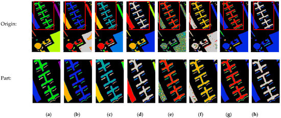
Figure 4. Clustering results obtained using different methods on the Pavia University data set. (a) Ground truth. (b) LRSC 46.16%. (c) SSC 64.27%. (d) S4C 66.72%. (e) EDSC 65.94%. (f) EGCSC 84.42%. (g) EKGCSC 97.32%. (h) SSAKGCSC 97.08%.

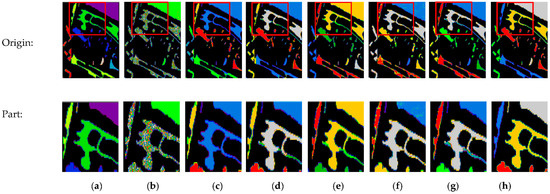
Figure 5. Clustering results obtained using different methods on the Pavia Center data set. (a) Ground truth. (b) LRSC 53.06%. (c) SSC 60.26%. (d) S4C 72.80%. (e) EDSC 75.39%. (f) EGCSC 80.30%. (g) EKGCSC 94.48%. (h) MEKGCSC 93.89%.

Table 3 shows the clustering performance comparison of different methods evaluated on SalinasA, Indian Pines, Pavia Center, and Pavia University data sets. From the results, it can be seen that the proposed methods achieve pretty adequate segmentation results on the HSI data sets without additional noise. It even outperforms the EKGCSC model in some aspects of OA, NMI, and Kappa coefficient. We can find a conspicuous progress in the performance of the traditional subspace clustering model with graph convolution from the SSAKGCSC significantly outperforming the EDSC results. Secondly, the SSAKGCSC algorithm that analyzes the nonlinear relationship between data points outperforms the EGCSC algorithm on all three data sets. That is, the GCSC algorithm with a nonlinear model can significantly improve the clustering performance by learning a more robust affinity matrix.

Table 3. Clustering performance of the compared methods on SalinasA, Indian Pines, Pavia University, and Pavia Center data sets.

Data	Metric	LRSC [19]	SSC [18]	S4C [14]	EDSC [24]	EGCSC [31]	EKGCSC [31]	SSAKGCSC
	OA	0.5009	0.7590	0.8070	0.8899	0.9993	1.0000	0.9989
SaA.	NMI	0.4657	0.7210	0.7563	0.8532	0.9971	1.0000	0.9960
	Kappa	0.4861	0.6953	0.7694	0.8327	0.9991	1.0000	0.9986
	OA	0.5752	0.5609	0.6497	0.7026	0.8827	0.9731	0.9743
InP.	NMI	0.5128	0.5081	0.6028	0.6544	0.6976	0.9128	0.9139
	Kappa	0.4566	0.4997	0.6325	0.6234	0.8308	0.9615	0.9632
	OA	0.4616	0.6427	0.6672	0.6594	0.8442	0.9732	0.9708
PaU.	NMI	0.4327	0.5994	0.6135	0.6252	0.8401	0.9482	0.9453
	Kappa	0.4425	0.5846	0.6047	0.6019	0.7968	0.9646	0.9538
	OA	0.5306	0.6026	0.7280	0.7539	0.8030	0.9448	0.9443
PaC.	NMI	0.4461	0.6801	0.7567	0.7873	0.8114	0.9252	0.9206
	Kappa	0.3773	0.4732	0.6401	0.6766	0.7447	0.9296	0.9289

The best results are highlighted in bold.

4.2.2. Images with Salt and Pepper Noise

Figure 6, Figure 7, Figure 8 and Figure 9 show the capability comparison of different clustering methods on the SalinasA, Indian Pines, Pavia Center, and Pavia University data sets with the addition of 0.1 probability of salt and pepper noise. As can be seen from Figure 5, the SSAKGCSC algorithm used in this work had a better performance compared to the EKGCSC algorithm in resisting salt and pepper noise. Since the EKGCSC algorithm cannot run on the noise-added PaviaU data set, the SSAKGCSC algorithm has better segmentation results compared to the rest of the comparison algorithms on the other two data sets.

Figure 6. Clustering results obtained using different methods on the SalinasA data set with salt and pepper noise. (a) Ground truth. (b) LRSC 43.49%. (c) SSC 48.60%. (d) S4C 51.08%. (e) EDSC 61.03%. (f) EGCSC 68.03%. (g) EKGCSC 45.74%. (h) SSAKGCSC 83.47%.

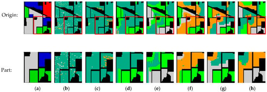
Figure 7. Clustering results obtained using different methods on the Indian Pines corrected data set with salt and pepper noise. (a) Ground truth. (b) LRSC 40.29%. (c) SSC 44.75%. (d) S4C 50.63%. (e) EDSC 52.88%. (f) EGCSC 57.07%. (g) EKGCSC 56.09%. (h) SSAKGCSC 66.34%.

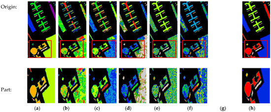
Figure 8. Clustering results obtained using different methods on the Pavia University data set with salt and pepper noise. (a) Ground truth. (b) LRSC 37.69%. (c) SSC 51.22%. (d) S4C 53.31%. (e) EDSC 53.56%. (f) EGCSC 60.12%. (g) EKGCSC. (h) SSAKGCSC 79.83%.

Figure 9. Clustering results obtained using different methods on the Pavia Center data set with salt and pepper noise. (a) Ground truth. (b) LRSC 38.21%. (c) SSC 50.39%. (d) S4C 52.38%. (e) EDSC 60.33%. (f) EGCSC 64.22%. (g) EKGCSC 33.68%. (h) MEKGCSC 85.01%.

Table 4 shows the performance comparison of different methods evaluated on SalinasA, Indian Pines, Pavia Center, and Pavia University data sets with the addition of a 0.1 probability of salt and pepper noise. From the results, it can be seen that the SSAKGCSC method used in this work achieves the best results in terms of both OA, NMI, and Kappa coefficients. In particular, the evaluation metrics on the SalinasA data set are almost double those of the EKGCSC model; on the other two data sets, our algorithm also shows a considerable improvement in three evaluation metrics. When the author runs the EKGCSC model for the PaviaU data set with noise, no matter whether it is pepper and salt noise or Gaussian noise, the program will be input the code segment of spectral clustering, so that its clustering result cannot be obtained no matter how long it runs.

Table 4. Clustering performance of the compared methods on SalinasA, Indian Pines, Pavia University, and Pavia Center data sets with salt and pepper noise (the probability is 0.1).

Data	Metric	LRSC [19]	SSC [18]	S4C [14]	EDSC [24]	EGCSC [31]	EKGCSC [31]	SSAKGCSC
	OA	0.4349	0.4860	0.5108	0.6103	0.6803	0.4574	0.8347
SaA.	NMI	0.4411	0.4413	0.5363	0.5827	0.7520	0.4331	0.8527
	Kappa	0.4157	0.4253	0.4634	0.5329	0.5781	0.2641	0.7905
	OA	0.4029	0.4475	0.5063	0.5288	0.5707	0.5609	0.6634
InP.	NMI	0.3564	0.3869	0.4016	0.4320	0.4330	0.4651	0.4665
	Kappa	0.2658	0.3186	0.3356	0.3534	0.3729	0.4151	0.5149
	OA	0.3769	0.5122	0.5331	0.5356	0.6012	-	0.7983
PaU.	NMI	0.4327	0.5994	0.6135	0.6252	0.8401	-	0.9453
	Kappa	0.4425	0.5846	0.6047	0.6019	0.7968	-	0.9538
	OA	0.3821	0.5039	0.5238	0.6033	0.6422	0.3368	0.8501
PaC.	NMI	0.4250	0.5281	0.5031	0.5833	0.6103	0.0382	0.8145
	Kappa	0.2318	0.3572	0.3817	0.5007	0.5537	0.0302	0.8103

The EKGCSC model will input the code segment of spectral clustering for the PaviaU data set with salt and pepper noise. The best results are highlighted in bold.

4.2.3. Images with Gaussian Noise

Figure 10, Figure 11, Figure 12 and Figure 13 show the clustering results of different clustering methods on the SalinasA, Indian Pines, Pavia Center, and Pavia University data sets under Gaussian noise with a mean of 0 and variance of 0.2. It can be seen from the results that the SSAKGCSC algorithm has an excellent performance in resisting Gaussian noise. This is especially evident in Figure 12, where the segmentation results of all the compared algorithms have a large area with noisy disturb, except for the result of the SSAKGCSC algorithm.

Figure 10. Clustering results obtained using different methods on the SalinasA data set with Gaussian noise. (a) Ground truth. (b) LRSC 35.96%. (c) SSC 47.61%. (d) S4C 54.77%. (e) EDSC 61.97%. (f) EGCSC 54.92%. (g) EKGCSC 60.73%. (h) SSAKGCSC 86.78%.

Figure 11. Clustering results obtained using different methods on the Indian Pines corrected data set with Gaussian noise. (a) Ground truth. (b) LRSC 43.20%. (c) SSC 42.20%. (d) S4C 53.29%. (e) EDSC 56.78%. (f) EGCSC 59.30%. (g) EKGCSC 54.70%. (h) SSAKGCSC 64.95%.

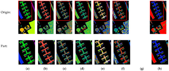
Figure 12. Clustering results obtained using different methods on the Pavia University data set with Gaussian noise. (a) Ground truth. (b) LRSC 36.90%. (c) SSC 36.79%. (d) S4C 42.51%. (e) EDSC 46.97%. (f) EGCSC 51.19%. (g) EKGCSC. (h) SSAKGCSC 67.34%.

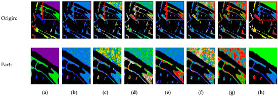
Figure 13. Clustering results obtained using different methods on the Pavia Center data set with Gaussian noise. (a) Ground truth. (b) LRSC 31.63%. (c) SSC 37.81%. (d) S4C 49.51%. (e) EDSC 47.57%. (f) EGCSC 48.44%. (g) EKGCSC 33.15%. (h) MEKGCSC 88.55%.

Table 5 shows the performance comparison of different clustering methods on the SalinasA, Indian Pines, Pavia Center, and Pavia University data sets under Gaussian noise with a mean of 0 and variance of 0.2. From the results, it can be seen that the SSAKGCSC method improves the OA, NMI, and Kappa coefficients by 26%, 24%, and 36%, respectively, compared to the standard method in the SalinasA data set. The method also improves the OA, NMI, and Kappa coefficients by 16%, 15%, and 16%, respectively, compared to the standard method in the Pavia University data set.

Table 5. Clustering performance of the compared methods on SalinasA, Indian Pines, Pavia University, and Pavia Center data sets with Gaussian noise (the mean is 0 and the variance is 0.2).

Data	Metric	LRSC [19]	SSC [18]	S4C [14]	EDSC [24]	EGCSC [31]	EKGCSC [31]	SSAKGCSC
	OA	0.3596	0.4761	0.5477	0.6197	0.5492	0.6073	0.8678
SaA.	NMI	0.3218	0.4536	0.5521	0.5747	0.6320	0.6639	0.9029
	Kappa	0.2764	0.4005	0.4353	0.4835	0.4180	0.4751	0.8310
	OA	0.4320	0.4220	0.5329	0.5678	0.5930	0.5470	0.6495
InP.	NMI	0.3169	0.3059	0.3563	0.5146	0.4148	0.3951	0.5348
	Kappa	0.2899	0.2744	0.3102	0.4837	0.4009	0.3774	0.4697
	OA	0.3690	0.3679	0.4251	0.4697	0.5119	-	0.6734
PaU.	NMI	0.3128	0.2843	0.3765	0.4167	0.4435	-	0.5902
	Kappa	0.2568	0.2363	0.2747	0.2858	0.3268	-	0.4807
	OA	0.3163	0.3781	0.4951	0.4757	0.4844	0.3315	0.8855
PaC.	NMI	0.0197	0.2883	0.5382	0.3404	0.4231	0.1612	0.8606
	Kappa	0.0028	0.1998	0.3629	0.2755	0.3459	0.1046	0.8537

The EKGCSC model will input the code segment of spectral clustering for the PaviaU data set with salt and pepper noise. The best results are highlighted in bold.

4.2.4. Images with Gaussian Noise and Salt and Pepper Noise

Figure 14, Figure 15, Figure 16 and Figure 17 show the performance comparison of different clustering methods on the SalinasA, Indian Pines, Pavia Center, and Pavia University data sets under both Gaussian noise with a mean of 0 and variance of 0.1 and salt and pepper noise with a probability of 0.1. It can be seen that the SSAKGCSC method still has the best classification results and remains to be the strongest among all algorithms for noise suppression. From the above, it can be concluded that the combined application of the GCSC framework, statistical sub-graph affinity model, and kernel function used in this research has adequate effectiveness and superiority in noise resistance of HSI segmentation.

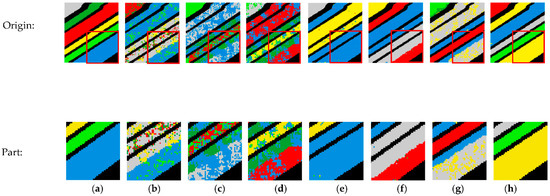
Figure 14. Clustering results obtained using different methods on the SalinasA data set with Gaussian noise and salt and pepper noise. (a) Ground truth. (b) LRSC 44.52%. (c) SSC 47.06%. (d) S4C 50.95%. (e) EDSC 60.79%. (f) EGCSC 62.23%. (g) EKGCSC 59.97%. (h) SSAKGCSC 88.28%.

Figure 15. Clustering results obtained using different methods on the Indian Pines corrected data set with Gaussian noise and salt and pepper noise. (a) Ground truth. (b) LRSC 41.08%. (c) SSC 43.86%. (d) S4C 51.33%. (e) EDSC 52.24%. (f) EGCSC 54.68%. (g) EKGCSC 52.49%. (h) SSAKGCSC 64.50%.

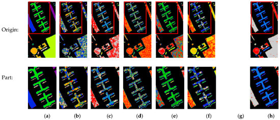
Figure 16. Clustering results obtained using different methods on the Pavia University data set with Gaussian noise and salt and pepper noise. (a) Ground truth. (b) LRSC 37.22%. (c) SSC 38.79%. (d) S4C 43.30%. (e) EDSC 47.91%. (f) EGCSC 50.92%. (g) EKGCSC. (h) SSAKGCSC 69.67%.

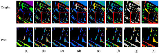
Figure 17. Clustering results obtained using different methods on the Pavia Center data set with Gaussian noise and salt and pepper noise. (a) Ground truth. (b) LRSC 34.17%. (c) SSC 42.89%. (d) S4C 47.94%. (e) EDSC 48.46%. (f) EGCSC 52.03%. (g) EKGCSC 31.82%. (h) MEKGCSC 88.72%.

Table 6 shows the performance comparison of different clustering methods on the SalinasA, Indian Pines, Pavia Center, and Pavia University data sets under Gaussian noise with a mean of 0 and variance of 0.1 and salt and pepper noise with a probability of 0.1. As can be seen from the table, the SSAKGCSC method improves the OA, NMI, and Kappa coefficients by 28%, 24%, and 36%, respectively, compared to the standard method in the SalinasA data set. The method also improves the OA, NMI, and Kappa coefficients by 19%, 16%, and 20%, respectively, compared to the standard method in the Pavia University data set.

Table 6. Clustering performance of the compared methods on SalinasA, Indian Pines, Pavia University, and Pavia Center data sets with Gaussian noise (the mean is 0 and the variance is 0.2) and salt and pepper noise (the probability is 0.1).

Data	Metric	LRSC [19]	SSC [18]	S4C [14]	EDSC [24]	EGCSC [31]	EKGCSC [31]	SSAKGCSC
	OA	0.4452	0.4706	0.5095	0.6079	0.6223	0.5997	0.8828
SaA.	NMI	0.3218	0.4536	0.5521	0.5747	0.6320	0.6639	0.9029
	Kappa	0.2764	0.4005	0.4353	0.4835	0.4180	0.4751	0.8310
	OA	0.4180	0.4386	0.5133	0.5224	0.5468	0.5249	0.6450
InP.	NMI	0.3169	0.3059	0.3563	0.4446	0.4148	0.3951	0.4958
	Kappa	0.2899	0.2744	0.3102	0.4837	0.4009	0.3774	0.4697
	OA	0.3722	0.3879	0.4330	0.4791	0.5092	-	0.6967
PaU.	NMI	0.3283	0.3247	0.3882	0.4082	0.4535	-	0.6102
	Kappa	0.2643	0.2695	0.3355	0.3564	0.3359	-	0.5338
	OA	0.3417	0.4289	0.4797	0.4846	0.5203	0.3182	0.8872
PaC.	NMI	0.1792	0.2270	0.3704	0.3434	0.5023	0.0451	0.8697
	Kappa	0.1999	0.2233	0.2668	0.3022	0.3895	0.130	0.8564

The EKGCSC model will input the code segment of spectral clustering for the PaviaU data set with salt and pepper noise. The best results are highlighted in bold.

4.3. Impact of the Number of PCs

Dimension reduction usually keeps the balance between computational efficiency and model performance. When more channels are taken into account, more specific information is included. However, possessing more channels does not always result in better clustering performance. To scientifically discuss the influence of the number of PCs, we implement the proposed methods with varying PCs from one to eight, then display the obtained OA and CPV in Figure 18. As shown in Figure 18, the clustering OA increased in the first four steps and then decreased. This appearance is known as the Hughes phenomenon [43], which is primarily due to increased correlation information and a lack of enough data points. As seen in Figure 18, the first four PCs of the data set can provide more than 96% of the CPV. This means that the remaining channels only possess restricted information and increase the risk of causing redundancy. Additionally, to identify subspaces correctly, the model must use more data points to model the statistical property of the data. To balance model accuracy with operational efficiency, we chose to use the first four PCs for the model.

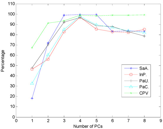
Figure 18. Clustering OA and CPV under a varying number of PCs on SalinasA, Indian Pines, Pavia Center and Pavia University data sets.

4.4. Comparison of Running Times

Table 7 shows the running times of our methods compared to the other competing methods. Since EGCSC, EKGCSC, and SSAKGCSC will achieve a closed-form solution without needing iterations, they are significantly quicker than LRSC, SSC, and S4C. Our method requires relatively more runtime compared to EDSC, which is because the GCSC framework requires constructing the graph from the original data points. Furthermore, SSAKGCSC needs to compute the sub-graph affinity matrix, so its running time will be increased compared to EGCSC and EKGCSC. In summary, our proposed SSAKGCSC model achieves a adequate balance between algorithm efficiency, clustering accuracy, and algorithm noise immunity.

Table 7. Running time of different methods (in seconds).

Data	LRSC [19]	SSC [18]	S4C [14]	EDSC [24]	EGCSC [31]	EKGCSC [31]	SSAKGCSC
SaA.	14,564	1832	19,865	85	200	340	588
InP.	8635	1341	3125	52	95	160	513
PaU.	32,764	2130	15,632	202	296	514	789
PaC.	20,354	1953	13,492	121	235	398	652

5. Discussion

In this paper, we introduced the HSI clustering framework based on graph convolution into subspace clustering (GCSC). The critical point of this framework is to use a graph convolution self-representation to integrate the intrinsic structural information of data points, followed by an explicit dictionary to learn robust affinity matrices. We also introduced statistical sub-graph affinity, a robust spectral clustering strategy to master the heavy noise, which constructs the affinity weighted graph based on the spatial intensity relationships between connected nodes. The statistical sub-graph affinity model includes a statistical noise model when treating the sub-graphs as random processes, thus better handling the uncertainty ingredient of noise. The statistical sub-graph affinity model contains neighborhood connectivity when representing the sub-graphs as random processes, thus making use of neighborhood information to counteract uncertainties and properties of noise. The experimental results on three HSI data sets show that the SSAKGCSC model can achieve the best performance compared to many existing clustering models. Moreover, the algorithm also has excellent performance over other algorithms in terms of noise immunity; in particular, the segmentation result on the SalinasA data set under salt and pepper noise is double than standard model EKGCSC, reaching 83.47%, 85.27%, and 79.05% of the clustering OA, NMI, Kappa coefficient, respectively.

6. Conclusions

The success of the SSAKGCSC model manifests that utilizing the intrinsic graph structure among data sets is crucial for clustering. The GCSC framework used in this study encourages us to implement traditional clustering models in non-Euclidean domains; this means that any improved tactics used in the classical subspace clustering model are suitable for GCSC. However, the GCSC framework suffers from quadratic complexity in the size of data points, which makes it difficult to be used for large-scale HSI data. In addition to the independent identically distributed noise model, other statistical models can be developed similarly. This paper illustrates statistical sub-graph affinity in image segmentation, which has an adequate ability to resist the additive noise.

First, future research will focus on how to effectively process the hyperspectral image with speckle noise, which is a multiplicative noise. Second, future work will focus on how to create the similarity matrix $W$ to more truly reflect the approximate relationship between data points. The Gaussian function used in this study has obvious limitations due to the selection of the scale parameter σ. A third future research aspect will explore how to automatically determine the number of clusters; although the number can be determined manually, it is a difficult problem to determine the exact number that has a direct effect on the efficiency and the final quality of clustering. Fourth, future work will look at how to select eigenvectors for the construction of new vector spaces, in most cases, the spectral clustering algorithm directly selects the first k maximum eigenvalues corresponding to the eigenvectors for the construction of new vector space. A final future research focus will investigate how to improve the running speed of spectral clustering and solve matrix eigenvalues and characteristic vectors. In dealing with large-scale data sets, the calculation of matrix space is very large; a solving process not only can be very time consuming but the required memory space is very large. Therefore, improving the running speed of the algorithm, reducing the memory space required to run, and reducing the time and space cost of the algorithm is another key problem in the process of expanding the application field of the algorithm.

References

- Ahmad, M.; Shabbir, S.; Roy, S.K.; Hong, D.; Wu, X.; Yao, J.; Khan, A.M.; Mazzara, M.; Distefano, S.; Chanussot, J. Hyperspectral Image Classification—Traditional to Deep Models: A Survey for Future Prospects. IEEE J. Sel. Top. Appl. Earth Obs. Remote Sens. 2022, 15, 968–999. [Google Scholar] [CrossRef]
- Cai, Y.; Dong, Z.; Cai, Z.; Liu, X.; Wang, G. Discriminative spectral-spatial attention-aware residual network for hyperspectral image classification. In Proceedings of the 10th Workshop on Hyperspectral Imaging and Signal Processing: Evolution in Remote Sensing (WHISPERS), Amsterdam, The Netherlands, 24–26 September 2019; pp. 1–5. [Google Scholar] [CrossRef]
- Xu, Z.; Yu, H.; Zheng, K.; Gao, L.; Song, M. A Novel Classification Framework for Hyperspectral Image Classification Based on Multiscale Spectral-Spatial Convolutional Network. In Proceedings of the 11th Workshop on Hyperspectral Imaging and Signal Processing: Evolution in Remote Sensing (WHISPERS), Amsterdam, The Netherlands, 24–26 March 2021; pp. 1–5. [Google Scholar] [CrossRef]
- Qin, A.; Shang, Z.; Tian, J.; Wang, Y.; Zhang, T.; Tang, Y.Y. Spectral–Spatial Graph Convolutional Networks for Semisupervised Hyperspectral Image Classification. IEEE Geosci. Remote Sens. Lett. 2018, 16, 241–245. [Google Scholar] [CrossRef]
- Li, S.; Song, W.; Fang, L.; Chen, Y.; Ghamisi, P.; Benediktsson, J.A. Deep Learning for Hyperspectral Image Classification: An Overview. IEEE Trans. Geosci. Remote Sens. 2019, 57, 6690–6709. [Google Scholar] [CrossRef]
- He, L.; Li, J.; Liu, C.; Li, S. Recent Advances on Spectral–Spatial Hyperspectral Image Classification: An Overview and New Guidelines. IEEE Trans. Geosci. Remote Sens. 2017, 56, 1579–1597. [Google Scholar] [CrossRef]
- Chairet, R.; Ben Salem, Y.; Aoun, M. Land cover classification of GeoEye image based on Convolutional Neural Networks. In Proceedings of the 2020 17th International Multi-Conference on Systems, Signals & Devices (SSD), Monastir, Tunisia, 20–23 July 2020; pp. 458–461. [Google Scholar] [CrossRef]
- Hu, P.; Liu, X.; Cai, Y.; Cai, Z. Band Selection of Hyperspectral Images Using Multiobjective Optimization-Based Sparse Self-Representation. IEEE Geosci. Remote Sens. Lett. 2018, 16, 452–456. [Google Scholar] [CrossRef]
- Chang, J.; Meng, G.; Wang, L.; Xiang, S.; Pan, C. Deep Self-Evolution Clustering. IEEE Trans. Pattern Anal. Mach. Intell. 2018, 42, 809–823. [Google Scholar] [CrossRef]
- Zhu, J.; Jiang, Z.; Evangelidis, G.D.; Zhang, C.; Pang, S.; Li, Z. Efficient registration of multi-view point sets by K-means clustering. Inf. Sci. 2019, 488, 205–218. [Google Scholar] [CrossRef]
- Zeng, M.; Cai, Y.; Cai, Z.; Liu, X.; Hu, P.; Ku, J. Unsupervised Hyperspectral Image Band Selection Based on Deep Subspace Clustering. IEEE Geosci. Remote Sens. Lett. 2019, 16, 1889–1893. [Google Scholar] [CrossRef]
- Zhang, L.; Zhang, L.; Du, B.; You, J.; Tao, D. Hyperspectral image unsupervised classification by robust manifold matrix factorization. Inf. Sci. 2019, 485, 154–169. [Google Scholar] [CrossRef]
- Yang, Y.; Wang, T. Kernel Subspace Clustering with Block Diagonal Prior. In Proceedings of the 2020 2nd International Conference on Machine Learning, Big Data and Business Intelligence (MLBDBI), Taiyuan, China, 23–25 October 2020; pp. 367–370. [Google Scholar] [CrossRef]
- Zhai, H.; Zhang, H.; Zhang, L.; Li, P.; Plaza, A. A New Sparse Subspace Clustering Algorithm for Hyperspectral Remote Sensing Imagery. IEEE Geosci. Remote Sens. Lett. 2017, 14, 43–47. [Google Scholar] [CrossRef]
- Wei, Y.; Niu, C.; Wang, Y.; Wang, H.; Liu, D. The Fast Spectral Clustering Based on Spatial Information for Large Scale Hyperspectral Image. IEEE Access 2019, 7, 141045–141054. [Google Scholar] [CrossRef]
- Tang, C.; Zhu, X.; Liu, X.; Li, M.; Wang, P.; Zhang, C.; Wang, L. Learning a Joint Affinity Graph for Multiview Subspace Clustering. IEEE Trans. Multimedia 2019, 21, 1724–1736. [Google Scholar] [CrossRef]
- Hinojosa, C.; Vera, E.; Arguello, H. A Fast and Accurate Similarity-Constrained Subspace Clustering Algorithm for Hyperspectral Image. IEEE J. Sel. Top. Appl. Earth Obs. Remote Sens. 2021, 14, 10773–10783. [Google Scholar] [CrossRef]
- Elhamifar, E.; Vidal, R. Sparse Subspace Clustering: Algorithm, Theory, and Applications. IEEE Trans. Pattern Anal. Mach. Intell. 2013, 35, 2765–2781. [Google Scholar] [CrossRef]
- Vidal, R.; Favaro, P. Low rank subspace clustering (LRSC). Pattern Recognit. Lett. 2013, 43, 47–61. [Google Scholar] [CrossRef]
- Patel, V.M.; Vidal, R. Kernel sparse subspace clustering. In Proceedings of the IEEE International Conference on Image Processing (ICIP), Paris, France, 27–30 October 2014; pp. 2849–2853. [Google Scholar] [CrossRef]
- Zhai, H.; Zhang, H.; Zhang, L.; Li, P. Laplacian-Regularized Low-Rank Subspace Clustering for Hyperspectral Image Band Selection. IEEE Trans. Geosci. Remote Sens. 2019, 57, 1723–1740. [Google Scholar] [CrossRef]
- Ji, P.; Salzmann, M.; Li, H. Efficient dense subspace clustering. In Proceedings of the IEEE Winter Conference on Applications of Computer Vision, Steamboat Springs, CO, USA, 24–26 March 2014; pp. 461–468. [Google Scholar] [CrossRef]
- Yang, X.; Xu, W.-D.; Liu, H.; Zhu, L.-Y. Research on Dimensionality Reduction of Hyperspectral Image under Close Range. In Proceedings of the 2019 International Conference on Communications, Information System and Computer Engineering (CISCE), Haikou, China, 5–7 July 2019; pp. 171–174. [Google Scholar] [CrossRef]
- Tian, L.; Du, Q.; Kopriva, I. L0-Motivated Low Rank Sparse Subspace Clustering for Hyperspectral Imagery. In Proceedings of the IEEE International Geoscience and Remote Sensing Symposium (IGARSS), Waikoloa, HI, USA, 26 September–2 October 2020; pp. 1038–1041. [Google Scholar] [CrossRef]
- Lu, C.; Feng, J.; Lin, Z.; Mei, T.; Yan, S. Subspace Clustering by Block Diagonal Representation. IEEE Trans. Pattern Anal. Mach. Intell. 2019, 41, 487–501. [Google Scholar] [CrossRef]
- Kipf, T.; Welling, M. Semi-supervised classification with graph convolutional networks. In Proceedings of the International Conference on Learning Representations, 9 September 2016; pp. 1–14. [Google Scholar] [CrossRef]
- Xu, H.; Yao, S.; Li, Q.; Ye, Z. An Improved K-means Clustering Algorithm. In Proceedings of the 2020 IEEE 5th International Symposium on Smart and Wireless Systems within the Conferences on Intelligent Data Acquisition and Advanced Computing Systems (IDAACS-SWS), Dortmund, Germany, 17–18 September 2020; pp. 1–5. [Google Scholar] [CrossRef]
- Zhu, Q.; Wang, Y.; Wang, F.; Song, M.; Chang, C.-I. Hyperspectral Band Selection Based on Improved Affinity Propagation. In Proceedings of the 11th Workshop on Hyperspectral Imaging and Signal Processing: Evolution in Remote Sensing (WHISPERS), Amsterdam, The Netherlands, 24–26 March 2021; pp. 1–4. [Google Scholar] [CrossRef]
- Pardo, A. Analysis of non-local image denoising methods. Pattern Recognit. Lett. 2011, 32, 2145–2149. [Google Scholar] [CrossRef]
- Fang, X.; Cai, Y.; Cai, Z.; Jiang, X.; Chen, Z. Sparse Feature Learning of Hyperspectral Imagery via Multiobjective-Based Extreme Learning Machine. Sensors 2020, 20, 1262. [Google Scholar] [CrossRef]
- Luo, B.; Wilson, R.C.; Hancock, E. Spectral embedding of graphs. Pattern Recognit. 2003, 36, 2213–2230. [Google Scholar] [CrossRef]
- Lei, T.; Jia, X.; Zhang, Y.; Liu, S.; Meng, H.; Nandi, A.K. Superpixel-Based Fast Fuzzy C-Means Clustering for Color Image Segmentation. IEEE Trans. Fuzzy Syst. 2019, 27, 1753–1766. [Google Scholar] [CrossRef]
- Yang, Y.; Gu, H.; Han, Y.; Li, H. An End-to-End Deep Learning Change Detection Framework for Remote Sensing Images. In Proceedings of the IEEE International Geoscience and Remote Sensing Symposium (IGARSS), Waikoloa, HI, USA, 26 September–2 October 2020; pp. 652–655. [Google Scholar] [CrossRef]
- Chang, J.; Oh, M.-H.; Park, B.-G. A systematic model parameter extraction using differential evolution searching. In Proceedings of the 2019 Silicon Nanoelectronics Workshop (SNW), Kyoto, Japan, 9–10 June 2019; pp. 1–2. [Google Scholar] [CrossRef]
- Kong, Y.; Cheng, Y.; Chen, C.L.P.; Wang, X. Hyperspectral Image Clustering Based on Unsupervised Broad Learning. IEEE Geosci. Remote Sens. Lett. 2019, 16, 1741–1745. [Google Scholar] [CrossRef]
- Eichel, J.A.; Wong, A.; Fieguth, P.; Clausi, D.A. Robust Spectral Clustering Using Statistical Sub-Graph Affinity Model. PLoS ONE 2013, 8, e82722. [Google Scholar] [CrossRef]
- JayaSree, M.; Rao, L.K. A Deep Insight into Deep Learning Architectures, Algorithms and Applications. In Proceedings of the 2022 International Conference on Electronics and Renewable Systems (ICEARS), Tuticorin, India, 16–18 March 2022; pp. 1134–1142. [Google Scholar] [CrossRef]
- Pan, Y.; Jiao, Y.; Li, T.; Gu, Y. An efficient algorithm for hyperspectral image clustering. In Proceedings of the IEEE International Conference on Acoustics, Speech and Signal Processing (ICASSP), Brighton, UK, 12–17 May 2019; pp. 2167–2171. [Google Scholar] [CrossRef]
- Cai, Y.; Zhang, Z.; Cai, Z.; Liu, X.; Jiang, X.; Yan, Q. Graph Convolutional Subspace Clustering: A Robust Subspace Clustering Framework for Hyperspectral Image. IEEE Trans. Geosci. Remote Sens. 2021, 59, 4191–4202. [Google Scholar] [CrossRef]
- Zeng, M.; Cai, Y.; Liu, X.; Cai, Z.; Li, X. Spectral–spatial clustering of hyperspectral image based on Laplacian regularized deep subspace clustering. In Proceedings of the IEEE International Geoscience and Remote Sensing Symposium (IGARSS), Yokohama, Japan, 28 July–2 August 2019; pp. 2694–2697. [Google Scholar] [CrossRef]
- Zhu, X.; Zhang, S.; Li, Y.; Zhang, J.; Yang, L.; Fang, Y. Low-Rank Sparse Subspace for Spectral Clustering. IEEE Trans. Knowl. Data Eng. 2019, 31, 1532–1543. [Google Scholar] [CrossRef]
- Wan, Y.; Zhong, Y.; Ma, A.; Zhang, L. Multi-Objective Sparse Subspace Clustering for Hyperspectral Imagery. IEEE Trans. Geosci. Remote Sens. 2020, 58, 2290–2307. [Google Scholar] [CrossRef]
- Gong, W.; Wang, Y.; Cai, Z.; Wang, L. Finding Multiple Roots of Nonlinear Equation Systems via a Repulsion-Based Adaptive Differential Evolution. IEEE Trans. Syst. Man, Cybern. Syst. 2020, 50, 1499–1513. [Google Scholar] [CrossRef]
Publisher’s Note: MDPI stays neutral with regard to jurisdictional claims in published maps and institutional affiliations. |
© 2022 by the authors. Licensee MDPI, Basel, Switzerland. This article is an open access article distributed under the terms and conditions of the Creative Commons Attribution (CC BY) license (https://creativecommons.org/licenses/by/4.0/).