Dynamics of an Impulsive Stochastic Predator–Prey System with the Beddington–DeAngelis Functional Response

Abstract

Taking impulsive effects into account, an impulsive stochastic predator–prey system with the Beddington–DeAngelis functional response is proposed in this paper. First, the impulsive system is transformed into an equivalent system without pulses. Then, by constructing suitable functionals and applying the extreme-value theory of quadratic functions, sufficient conditions on the existence of periodic Markovian processes are provided. The uniform continuity and global attractivity of solutions are also investigated. Additionally, we investigate the extinction and permanence in the mean of all species with the help of comparison methods and inequality techniques. Sufficient conditions on the existence and ergodicity of the stationary distribution of solutions for the autonomous and non-impulsive case are given. Finally, numerical simulations are performed to illustrate the main results.

1. Introduction

Predator–prey systems with the Beddington–DeAngelis functional response have always attracted the attention of many researchers (to name a few, see [1,2,3] and the references therein). As we know, white noises are very common in the real world. They affect the growth rates of species to some extent. In order to understand the effects of white noises on the dynamics of ecological systems, random disturbance is introduced [4,5,6,7,8,9]. For example, Yagi and Ton [9] studied the following model:

$$\left\{\begin{array}{ccc}\hfill d{x}_1\left(t\right)& =& x_1\left(t\right)\left({\displaystyle a_{11}\left(t\right)-a_{12}\left(t\right)x_1\left(t\right)-\frac{c_1\left(t\right)x_2\left(t\right)}{m_0\left(t\right)+m_1\left(t\right)x_1\left(t\right)+m_2\left(t\right)x_2\left(t\right)}}\right)dt\hfill \\ & & +{\sigma }_1\left(t\right)x_1\left(t\right)d{\omega }_1\left(t\right),\hfill \\ \hfill d{x}_2\left(t\right)& =& x_2\left(t\right)\left({\displaystyle -a_{21}\left(t\right)-a_{22}\left(t\right)x_2\left(t\right)+\frac{c_2\left(t\right)x_1\left(t\right)}{m_0\left(t\right)+m_1\left(t\right)x_1\left(t\right)+m_2\left(t\right)x_2\left(t\right)}}\right)dt\hfill \\ & & +{\sigma }_2\left(t\right)x_2\left(t\right)d{\omega }_2\left(t\right),\hfill \end{array}\right.$$

(1)

where $x_1\left(t\right)$ and $x_2\left(t\right)$ represent the quantities of prey and predator populations, respectively; ${\omega }_1\left(t\right)$ and ${\omega }_2\left(t\right)$ are independent standard Brownian motions defined on the complete probability space $(\mathsf{\Omega },F,{\left\{F_t\right\}}_{t\ge 0},P)$ with a filtration ${\left\{F_t\right\}}_{t\ge 0}$ satisfying the usual conditions—that is, it is increasing and right continuous and $F_0$ contains all P-null set. See [1,3] for the biological meanings of the parameter functions.

Moreover, the growths of species usually suffer rapid changes in relatively short time periods due to activities such as stocking and harvesting. To describe such phenomena, impulsive dynamical systems have been proposed and studied (e.g., [10,11,12,13,14,15] and references therein).

Furthermore, the life cycles of species and the variation of the environment play important roles in many biological and ecological dynamical systems. In particular, the effects of a periodically varying environment are important for evolutionary theory, as the selective forces on systems in a fluctuating environment differ from those in a stable environment. Therefore, the assumption of periodicity on parameters in the system (in a way) incorporates the periodicity of the environment [16,17,18].

Motivated by the above discussion and based on (1), we propose the following periodic impulsive stochastic predator–prey model with the Beddington–DeAngelis functional response:

$$\left\{\begin{array}{c}\left.\begin{array}{ccc}\hfill d{x}_1\left(t\right)& =& x_1\left(t\right)\left({\displaystyle a_{11}\left(t\right)-a_{12}\left(t\right)x_1\left(t\right)-\frac{c_1\left(t\right)x_2\left(t\right)}{m_0\left(t\right)+m_1\left(t\right)x_1\left(t\right)+m_2\left(t\right)x_2\left(t\right)}}\right)dt\hfill \\ & & +{\sigma }_1\left(t\right)x_1\left(t\right)d{\omega }_1\left(t\right),\hfill \\ \hfill d{x}_2\left(t\right)& =& x_2\left(t\right)\left({\displaystyle -a_{21}\left(t\right)-a_{22}\left(t\right)x_2\left(t\right)+\frac{c_2\left(t\right)x_1\left(t\right)}{m_0\left(t\right)+m_1\left(t\right)x_1\left(t\right)+m_2\left(t\right)x_2\left(t\right)}}\right)dt\hfill \\ \hfill & & +{\sigma }_2\left(t\right)x_2\left(t\right)d{\omega }_2\left(t\right),\hfill \end{array}\right\}t\ne t_k,\hfill \\ \\ \left.\begin{array}{ccc}\hfill x_1\left(t_k^{+}\right)& =& (1+{\xi }_{1k})x_1\left(t_k\right),\hfill \\ \hfill x_2\left(t_k^{+}\right)& =& (1+{\xi }_{2k})x_2\left(t_k\right),\hfill \end{array}\right\}t=t_k.\hfill \end{array}\right.$$

(2)

In the sequel, we always assume that the following conditions are satisfied by the constants and parameter functions of (2).

• All functions $a_{11}(·)$, $a_{12}(·)$, $a_{21}(·)$, $a_{22}(·)$, $c_1(·)$, $c_2(·)$, $m_0(·)$, $m_1(·)$, $m_2(·)$, ${\sigma }_1(·)$, and ${\sigma }_2(·)$ are positive, bounded, continuous, and periodic with the same period T.
• The impulsive points satisfy $0<t_1<t_2<\cdots$ with ${lim}_{k\to \infty }{t}_k=\infty$ and there exists a positive integer q such that $t_{k+q}=t_k+T$ and ${\xi }_{i,k+q}={\xi }_{i,k}$ for $i=1$, 2 and $k\in N=\{1,2,\dots \}$.
• By the biological meanings, we assume ${\xi }_{ik}>-1$ for $i=1$, 2 and $k\in N=\{1,2,\dots \}$.

The motivations for investigating the dynamics of (2) are as follows. Firstly, for deterministic systems, the existence and attractivity of equilibria/periodic solutions are important topics for understanding the dynamics of ecological systems [19,20,21,22,23]. Similarly, for stochastic systems, it is crucial to study the existence of periodic Markovian processes. Secondly, extinction, permanence in mean for all species, and stochastic persistence are all important properties to understand the dynamics of biological systems [24,25,26,27]. Lastly, for the special case of (2) with parameter functions being constants, it is interesting to study the existence of a stationary distribution as the functional response is non-monotonic.

The rest of this paper is organized as follows. Section 2 begins with definitions, important lemmas, and some notations. Section 3 provides sufficient conditions on the existence of periodic Markovian processes for (2). Section 4 focuses on the extinction and permanence in the mean of all species of (2). Section 6 is devoted to the existence and uniqueness of distribution. Some numerical simulations are given in Section 7. The paper concludes with a brief discussion and conclusions.

2. Preliminaries

We start with the definition of a periodic Markovian process.

Definition 1

([9,18]). A stochastic process $\xi \left(t\right)=\xi (t,\omega )$$(-\infty <t<\infty )$ is said to be periodic with period T if for every finite sequence of numbers $t_1$, $t_2$, …, $t_n$ the joint distribution of the random variables $\xi (t_1+h)$, …, $\xi (t_n+h)$ is independent of h, where $h=kT$ with $k=\pm 1$, $\pm 2$, …

Definition 2

([13,15]). For the following impulsive stochastic system of differential equations:

$$\left\{\begin{array}{ccc}\hfill dx\left(t\right)& =& f(t,x\left(t\right))dt+g(t,x\left(t\right))d\omega \left(t\right),t\ne t_k,\hfill \\ \hfill x\left(t_k^{+}\right)& =& (1+{\lambda }_k)x\left(t_k\right),k\in N,\hfill \end{array}\right.$$

(3)

with the initial value $x\left(0\right)=x_0\in R^n$, a stochastic process $x\left(t\right)={(x_1\left(t\right),x_2\left(t\right),\dots ,x_n\left(t\right))}^T$, $t\in R_{+}=[0,\infty )$ is said to be a solution if

(i) 

$x\left(t\right)$ is $f_t$-adapted and is continuous on $(0,t_1)$ and each interval $(t_k,t_{k+1})\subset R_{+}, k\in N$, $f(t,x\left(t\right))\in L(R_{+},R^n), g(t,x\left(t\right))\in L^2(R_{+},R^n)$, where $L^p(R_{+},R^n)$ is the set of all $R^n$-valued measurable $f_t$-adapted processes satisfying ${\int }_0^T{\left|f\left(t\right)\right|}^{p}dt<\infty$ almost surely for all $T>0$,$p=1$, 2;

(ii) 

For every $t_k$, $k\in N$, $x\left(t_k^{+}\right)={lim}_{t\to t_k^{+}}x\left(t\right)$ and $x\left(t_k^{-}\right)={lim}_{t\to t_k^{-}}x\left(t\right)$ exist, and $x\left(t_k\right)=x\left(t_k^{-}\right)$ with the probability one;

(iii) 

For all $t\in [0,t_1], x\left(t\right)$ obeys the integral equation

$$x\left(t\right)=x\left(0\right)+{\int }_0^{t}f(s,x\left(s\right))ds+{\int }_0^{t}g(s,x\left(s\right))d\omega \left(s\right)$$

and for all $t\in [t_k,t_{k+1}], k\in N, x\left(t\right)$ obeys the following integral equation:

$$x\left(t\right)=x\left(t_k^{+}\right)+{\int }_{t_k}^{t}f(s,x\left(s\right))ds+{\int }_{t_k}^{t}g(s,x\left(s\right))d\omega \left(s\right).$$

Definition 3

([27]). System (2) is globally attractive if

$$\underset{t\to \infty }{lim}|x_1\left(t\right)-{\tilde{x}}_1\left(t\right)|=\underset{t\to \infty }{lim}|x_2\left(t\right)-{\tilde{x}}_2\left(t\right)|=0$$

for any two positive solutions $(x_1\left(t\right),x_2\left(t\right))$ and $({\tilde{x}}_1\left(t\right),{\tilde{x}}_2\left(t\right))$.

Lemma 1

([15]). For the following Itô’s differential equation:

$$dx\left(t\right)=b(t,x(t\left)\right)dt+\sigma (t,x(t\left)\right)d\omega \left(t\right),$$

(4)

if all the coefficients are T-periodic in t and satisfy the linear growing condition and the Lipschitz condition in every cylinder $U_l\times R_{+}$ for $l>0$, where $U_l=\{x:|\left|x\right||\le l\}$ and there exists a function $v=v(t,x)$ which is twice continuously differentiable with respect to x and continuously differentiable with respect to t in $R^n\times R_{+},$ T-periodic in t and satisfies the following conditions:

$$\underset{\left|\right|x\left|\right|>l}{inf}v(t,x)\to \infty asl\to \infty ,$$

$$Lv(t,x)\le -1outside some compact set,$$

then there exists a solution of (4) which is a T-periodic Markovian process, where L is the generator of (4) defined by

$$Lv(t,x)=\left[\frac{\partial v}{\partial t}+{\nabla }_{x}v·b+0.5tr\left(\sigma {\sigma }^T{v}_{xx}\right)\right](t,x).$$

Lemma 2

([13]). Suppose that $Z\in C(R_{+},(0,\infty ))$ and $\underset{t\to \infty }{lim}F\left(t\right)/t=0$ a.s.

(a) 

If there exist two positive constants $t_0>0$ and ${\lambda }_0>0$ such that, for all $t>t_0$,

$$lnZ\left(t\right)\le \lambda t-{\lambda }_0{\int }_0^{t}z\left(s\right)ds+F\left(t\right)a.s.,$$

then

$$\left\{\begin{array}{ccc}\hfill {⟨Z⟩}^{*}& \le & \lambda /{\lambda }_{0}a.s.if\lambda \ge 0,\hfill \\ \hfill \underset{t\to \infty }{lim}Z\left(t\right)& =& 0a.s.if\lambda <0.\hfill \end{array}\right.$$

(b) 

If there exist some constants $t_0>0$, ${\lambda }_0>0$, and λ such that, for all $t>t_0$,

$$lnZ\left(t\right)\ge \lambda t-{\lambda }_0{\int }_0^{t}z\left(s\right)ds+F\left(t\right)a.s.,$$

then

$${⟨Z⟩}_{*}\ge \lambda /{\lambda }_{0}a.s.$$

Lemma 3

([28]). Suppose that an n-dimensional stochastic process $x\left(t\right)$ on $t\ge 0$ satisfies

$${\mathbb{E}|x\left(t\right)-x\left(s\right)|}^{{\beta }_1}\le c{|t-s|}^{1+{\beta }_2},0\le s,t<\infty ,$$

for some positive constants ${\beta }_1$, ${\beta }_2$, and c. Then there exists a continuous modification $\tilde{x}\left(t\right)$ of $x\left(t\right)$, which has the property that, for every $\vartheta \in (0,\frac{{\beta }_2}{{\beta }_1}),$ there is a positive random variable $h\left(\omega \right)$ such that

$$P\left\{\omega :\underset{0<|t-s|<h\left(\omega \right),0\le s,t<\infty }{sup}\frac{|\tilde{x}(t,\omega )-x(t,\omega )|}{{|t-s|}^{\vartheta }}\le \frac{2}{1-2^{-\vartheta }}\right\}=1.$$

In other words, almost every sample path of $\tilde{x}\left(t\right)$ is locally but uniformly Hölder continuous with exponent ϑ.

Lemma 4

([29]). Let f be a nonnegative function defined on $R_{+}$ such that f is integrable on $R_{+}$ and is uniformly continuous on $R_{+}$, then $\underset{t\to \infty }{lim}f\left(t\right)=0$.

To investigate the dynamics of (2), we first consider the following non-impulsive system:

$$\left\{\begin{array}{ccc}\hfill d{y}_1\left(t\right)& =& {\displaystyle y_1\left(t\right)(a_{11}\left(t\right)+\frac{1}{T}\sum _{j=1}^{q}ln(1+{\xi }_{1k})-a_{12}\left(t\right)A_1\left(t\right)y_1\left(t\right)}\hfill \\ & & {\displaystyle -\frac{c_1\left(t\right)A_2\left(t\right)y_2\left(t\right)}{m_0\left(t\right)+m_1\left(t\right)A_1\left(t\right)y_1\left(t\right)+m_2\left(t\right)A_2\left(t\right)y_2\left(t\right)})dt+{\sigma }_1\left(t\right)y_1\left(t\right)d{\omega }_1\left(t\right),}\hfill \\ \\ \hfill d{y}_2\left(t\right)& =& {\displaystyle y_2\left(t\right)(-a_{21}\left(t\right)+\frac{1}{T}\sum _{j=1}^{q}ln(1+{\xi }_{2k})-a_{22}\left(t\right)A_2\left(t\right)y_2\left(t\right)}\hfill \\ & & {\displaystyle +\frac{c_2\left(t\right)A_1\left(t\right)y_1\left(t\right)}{m_0\left(t\right)+m_1\left(t\right)A_1\left(t\right)y_1\left(t\right)+m_2\left(t\right)A_2\left(t\right)y_2\left(t\right)})dt+{\sigma }_2\left(t\right)y_2\left(t\right)d{\omega }_2\left(t\right),}\hfill \end{array}\right.$$

(5)

where

$$A_i\left(t\right)={\left[\prod _{j=1}^q(1+{\xi }_{ij})\right]}^{-\frac{t}{T}}\prod _{0\le t_k<t}(1+{\xi }_{ik}),i=1,2,$$

with the convention that the product of an empty index set is 1. It is easy to show that both $A_1(·)$ and $A_2(·)$ are T-periodic. We refer the readers to [22] for details.

Lemma 5.

Let $x_1\left(t\right)=A_1\left(t\right)y_1\left(t\right)$ and $x_2\left(t\right)=A_2\left(t\right)y_2\left(t\right)$. Then the following two statements hold.

(i) 

If $y\left(t\right)=(y_1\left(t\right),y_2\left(t\right))$ is a solution of (5), then $x\left(t\right)=(x_1\left(t\right),x_2\left(t\right))$ is a solution of (2);

(ii) 

If $x\left(t\right)=(x_1\left(t\right),x_2\left(t\right))$ is a solution of (2), then $y\left(t\right)=(y_1\left(t\right),y_2\left(t\right))$ is a solution of (5).

The assertions in Lemma 5, similar to Theorem 3.1 in [13], follow easily from Definition 2 and hence the proof is omitted here. Lemma 5 tells us that when the dynamics of (2) is considered, it suffices to focus on that of (5).

With similar arguments as those in the proof of Theorem 2.1 in [26], we can obtain the existence and non-negativeness of solutions to (5).

Theorem 1.

For any given initial value $(y_1\left(0\right),y_2\left(0\right))\in R_{+}^2$, (5) has a unique solution $(y_1\left(t\right),y_2\left(t\right))$ on $R_{+}$ with $(y_1\left(t\right),y_2\left(t\right))\in R_{+}^2$ for $t\in R_{+}$ with probability one.

Finally, for any positive, bounded, and continuous function $f(·)$ on $R_{+}$, we denote

$$f^u=sup\{f\left(t\right),t\ge 0\},f^l=inf\{f\left(t\right),t\ge 0\},f^{*}=\underset{t\to \infty }{lim\; sup}f\left(t\right),f_{*}=\underset{t\to \infty }{lim\; inf}f\left(t\right).$$

If $f(·)$ is further integrable, then

$$⟨f⟩=\underset{t\to \infty }{lim}\frac{1}{t}{\int }_0^{t}f\left(s\right)dsand{⟨f⟩}_T=\frac{1}{T}{\int }_0^{T}f\left(s\right)ds.$$

3. Existence of Periodic Markovian Processes

In this section, we first study the existence of periodic Markovian processes of (5).

Theorem 2.

Suppose the following condition $\left(H_1\right)$ holds,

$$\left(H_1\right)\begin{array}{ccc}\hfill {\lambda }_{\mathrm{T}}:& =& {\displaystyle {⟨{\displaystyle m_2^l{a}_{11}\left(t\right)-c_1\left(t\right)-a_{21}\left(t\right)-\frac{m_2^l{\sigma }_1^2\left(t\right)+{\sigma }_2^2\left(t\right)}{2}}⟩}_T+\frac{m_2^l}{T}\sum _{j=1}^{q}ln(1+{\xi }_{1k})+\frac{1}{T}\sum _{j=1}^{q}ln(1+{\xi }_{2k})}\hfill \\ & >& max\left\{{\displaystyle \frac{{(A_2^u{a}_{22}^u-c_1^l{A}_2^l{a}_{21}^l)}^2}{4c_1^l{\left(A_2^l\right)}^2{a}_{22}^l},\frac{{\left(A_1^u(c_2^u{a}_{11}^u+m_2^l{a}_{12}^u)\right)}^2}{4c_2^u{a}_{12}^l{A}_1^u{A}_1^l}}\right\}.\hfill \end{array}$$

Then there exists at least one positive T-Markovian process for (5).

Proof. 

It suffices to find a $C^2$-function $V(t,y_1,y_2)$ and a closed set $U\subset R_{+}^2$ such that all conditions of Lemma 1 hold. Define

$$V_1(t,y_1)=c_2^u{A}_1^u{y}_1-m_2^{l}ln{y}_1,V_2\left(y_2\right)=c_1^l{A}_2^l{y}_2-ln{y}_2,$$

and $V(t,y_1,y_2)=V_1(t,y_1)+V_2(t,y_2)+W\left(t\right),$ where $W\left(t\right)$ is a positive differentiable function satisfying

$$W^{\prime }\left(t\right)=m_2^l{a}_{11}\left(t\right)-c_1\left(t\right)-a_{21}\left(t\right)-\frac{m_2^l{\sigma }_1^2\left(t\right)+{\sigma }_2^2\left(t\right)}{2}-{⟨m_2^l{a}_{11}\left(t\right)-c_1\left(t\right)-a_{21}\left(t\right)-\frac{m_2^l{\sigma }_1^2\left(t\right)+{\sigma }_2^2\left(t\right)}{2}⟩}_T.$$

It is not difficult to verify that $W\left(t\right)$ is a T-periodic function on $R_{+}$ and

$$\underset{(y_1,y_2)\in R_{+}^2/U_k}{lim\; inf}V(t,y_1,y_2)\to \infty ask\to \infty ,$$

where $U_k=\{(y_1,y_2):(y_1,y_2)\in (\frac{1}{k},k)\times (\frac{1}{k},k)\}$. Hence $V(t,y_1,y_2)$ is T-periodic and satisfies the first condition of Lemma 1. Next we verify the second condition of Lemma 1. Applying Itô’s formula to $V_1(t,y_1)$ and $V_2(t,y_2)$ gives

$$\begin{array}{ccc}\hfill L{V}_1(t,y_1)& =& {\displaystyle \left({\displaystyle c_2^u{A}_1^u-\frac{m_2^l}{y_1}}\right)y_1(a_{11}\left(t\right)+\frac{1}{T}\sum _{j=1}^{q}ln(1+{\xi }_{1k})-a_{12}\left(t\right)A_1\left(t\right)y_1}\hfill \\ & & {\displaystyle -\frac{c_1\left(t\right)A_2\left(t\right)y_2}{m_0\left(t\right)+m_1\left(t\right)A_1\left(t\right)y_1+m_2\left(t\right)A_2\left(t\right)y_2})+\frac{m_2^l{\sigma }_1^2\left(t\right)}{2}}\hfill \\ & \le & -m_2^l\left({\displaystyle a_{11}\left(t\right)+\frac{1}{T}\sum _{j=1}^{q}ln(1+{\xi }_{1k})-\frac{{\sigma }_1^2\left(t\right)}{2}}\right)\hfill \\ & & {\displaystyle +m_2^l\frac{c_1\left(t\right)A_2\left(t\right)y_2}{m_0\left(t\right)+m_1\left(t\right)A_1\left(t\right)y_1+m_2\left(t\right)A_2\left(t\right)y_2}}\hfill \\ & & {\displaystyle -c_2^u{A}_1^u\frac{c_1^l{A}_2^l{y}_1{y}_2}{m_0\left(t\right)+m_1\left(t\right)A_1\left(t\right)y_1+m_2\left(t\right)A_2\left(t\right)y_2}}\hfill \\ & & +(m_2^l{a}_{12}\left(t\right)A_1\left(t\right)+c_2^u{A}_1^u{a}_{11}\left(t\right))y_1-c_2^u{A}_1^u{a}_{12}\left(t\right)A_1\left(t\right)y_1^2,\hfill \end{array}$$

and

$$\begin{array}{ccc}\hfill L{V}_2(t,y_2)& =& {\displaystyle \left({\displaystyle c_1^l{A}_2^l-\frac{1}{y_2}}\right)y_2(-a_{21}\left(t\right)+\frac{1}{T}\sum _{j=1}^{q}ln(1+{\xi }_{2k})-a_{22}\left(t\right)A_2\left(t\right)y_2}\hfill \\ & & {\displaystyle +\frac{c_2\left(t\right)A_1\left(t\right)y_1}{m_0\left(t\right)+m_1\left(t\right)A_1\left(t\right)y_1+m_2\left(t\right)A_2\left(t\right)y_2})+\frac{{\sigma }_2^2\left(t\right)}{2}}\hfill \\ & \le & \left({\displaystyle a_{21}\left(t\right)-\frac{1}{T}\sum _{j=1}^{q}ln(1+{\xi }_{2k})+\frac{{\sigma }_2^2\left(t\right)}{2}}\right)\hfill \\ & & {\displaystyle +c_1^l{A}_2^l\frac{c_2^u{A}_1^u{y}_1{y}_2}{m_0\left(t\right)+m_1\left(t\right)A_1\left(t\right)y_1+m_2\left(t\right)A_2\left(t\right)y_2}}\hfill \\ & & {\displaystyle -c_2\left(t\right)A_1\left(t\right)\frac{y_1}{m_0\left(t\right)+m_1\left(t\right)A_1\left(t\right)y_1+m_2\left(t\right)A_2\left(t\right)y_2}}\hfill \\ & & +(a_{22}\left(t\right)A_2\left(t\right)-c_1^l{A}_2^l{a}_{21}\left(t\right))y_2-c_1^l{A}_2^l{a}_{22}\left(t\right)A_2\left(t\right)y_2^2,\hfill \end{array}$$

respectively. Then

$$\begin{array}{ccc}\hfill LV& \le & -m_2^l\left({\displaystyle a_{11}\left(t\right)+\frac{1}{T}\sum _{j=1}^{q}ln(1+{\xi }_{1k})-\frac{{\sigma }_1^2\left(t\right)}{2}}\right)+\left({\displaystyle a_{21}\left(t\right)+\frac{{\sigma }_2^2\left(t\right)}{2}-\frac{1}{T}\sum _{j=1}^{q}ln(1+{\xi }_{2k})}\right)\hfill \\ & & {\displaystyle +\frac{m_2^l{c}_1\left(t\right)A_2\left(t\right)y_2}{m_0\left(t\right)+m_1\left(t\right)A_1\left(t\right)y_1+m_2\left(t\right)A_2\left(t\right)y_2}+W^{\prime }\left(t\right)+(c_2^u{A}_1^u{a}_{11}\left(t\right)+m_2^l{a}_{12}\left(t\right)A_1\left(t\right))y_1}\hfill \\ & & -c_2^u{A}_1^u{a}_{12}\left(t\right)A_1\left(t\right)y_1^2+(a_{22}\left(t\right)A_2\left(t\right)-c_1^l{A}_2^l{a}_{21}\left(t\right))y_2-c_1^l{A}_2^l{a}_{22}\left(t\right)A_2\left(t\right)y_2^2\hfill \\ & \le & -{\lambda }_T-c_2^u{A}_1^u{a}_{12}^l{A}_1^l{y}_1^2+A_1^u(c_2^u{a}_{11}^u+m_2^l{a}_{12}^u)y_1\hfill \\ & & -c_1^l{A}_2^l{a}_{22}^l{A}_2^l{y}_2^2+(A_2^u{a}_{22}^u-c_1^l{A}_2^l{a}_{21}^l)y_2.\hfill \end{array}$$

Choose $\epsilon \in (0,1)$ such that

$$\begin{array}{ccc}\hfill \frac{1}{2}\left\{{\lambda }_T-\frac{{(A_2^u{a}_{22}^u-c_1^l{A}_2^l{a}_{21}^l)}^2}{4c_1^l{\left(A_2^l\right)}^2{a}_{22}^l}\right\}& >& A_1^u(c_2^u{a}_{11}^u+m_2^l{a}_{12}^u)\epsilon ,\hfill \\ \hfill \frac{1}{2}\left\{{\displaystyle {\lambda }_T-\frac{{\left(A_1^u(c_2^u{a}_{11}^u+m_2^l{a}_{12}^u)\right)}^2}{4c_2^u{a}_{12}^l{A}_1^u{A}_1^l}}\right\}& >& (A_2^u{a}_{22}^u-c_1^l{A}_2^l{a}_{21}^l)\epsilon ,\hfill \end{array}$$

(6)

$$\begin{array}{ccc}\hfill -c_2^u{A}_1^u{a}_{12}^l{A}_1^l{y}_1^2+A_1^u(c_2^u{a}_{11}^u+m_2^l{a}_{12}^u)y_1& <& -\frac{1}{2}\mathrm{for} y_1>\frac{1}{\epsilon },\hfill \\ \hfill -c_1^l{A}_2^l{a}_{22}^l{A}_2^l{y}_2^2+(A_2^u{a}_{22}^u-c_1^l{A}_2^l{a}_{21}^l)y_2& <& -\frac{1}{2}\mathrm{for} y_2>\frac{1}{\epsilon }.\hfill \end{array}$$

(7)

Denote

$$D_{\epsilon }=\left\{(y_1,y_2):(y_1,y_2)\in [\epsilon ,\frac{1}{\epsilon }]\times [\epsilon ,\frac{1}{\epsilon }]\right\}.$$

Then $D_{\epsilon }$ is compact and its complement $D_{\epsilon }^C=R_{+}^2/D_{\epsilon }={\displaystyle \bigcup _{i=1}^4}{D}_{\epsilon }^i$, where

$$\begin{array}{ccc}\hfill D_{\epsilon }^1=\{(y_1,y_2)\in R_{+}^2|y_1<\epsilon \},& & D_{\epsilon }^2=\{(y_1,y_2)\in R_{+}^2|y_2<\epsilon \},\hfill \\ \hfill D_{\epsilon }^3=\{(y_1,y_2)\in R_{+}^2|y_1>\frac{1}{\epsilon }\},& & D_{\epsilon }^4=\{(y_1,y_2)\in R_{+}^2|y_2>\frac{1}{\epsilon }\}.\hfill \end{array}$$

Accordingly, we distinguish four cases to finish the proof.

Case (i): $(y_1,y_2)\in D_{\epsilon }^1$. Note that

$$-c_1^l{\left(A_2^l\right)}^2{a}_{22}^l{y}_2^2+(A_2^u{a}_{22}^u-c_1^l{A}_2^l{a}_{21}^l)y_2\le \frac{{(A_2^u{a}_{22}^u-c_1^l{A}_2^l{a}_{21}^l)}^2}{4c_1^l{\left(A_2^l\right)}^2{a}_{22}^l}.$$

(8)

By (6), we get

$$LV\le -\frac{1}{2}\left\{{\lambda }_T-\frac{{(A_2^u{a}_{22}^u-c_1^l{A}_2^l{a}_{21}^l)}^2}{4c_1^l{\left(A_2^l\right)}^2{a}_{22}^l}\right\}<0.$$

Case (ii): $(y_1,y_2)\in D_{\epsilon }^2$. Similar to Case (i), we can get

$$LV\le -\frac{1}{2}\left\{{\displaystyle {\lambda }_T-\frac{{\left(A_1^u(c_2^u{a}_{11}^u+m_2^l{a}_{12}^u)\right)}^2}{4c_2^u{a}_{12}^l{A}_1^u{A}_1^l}}\right\}<0.$$

Case (iii): $(y_1,y_2)\in D_{\epsilon }^3$. In this case, by (8) and the definition of ${\lambda }_T$ and the choice of $\epsilon$, we have

$$LV\le -{\lambda }_T-\frac{1}{2}+\frac{{(A_2^u{a}_{22}^u-c_1^l{A}_2^l{a}_{21}^l)}^2}{4c_1^l{\left(A_2^l\right)}^2{a}_{22}^l}\le -\frac{1}{2}.$$

Case (iv): $(y_1,y_2)\in D_{\epsilon }^4$. Similar to case (iii), we can show that

$$LV\le -\frac{1}{2}.$$

In summary, we have verified the second condition of Lemma 1. This completes the proof. □

Before proving the global attractivity of (5), we first study its boundedness and uniform continuity.

Lemma 6.

For any initial value $y\left(0\right)={(y_1\left(0\right),y_2\left(0\right))}^T\in R_{+}^2$, the solution $(y_1\left(t\right),y_2\left(t\right))$ of (5) satisfies

$$\underset{t\to \infty }{lim\; sup}\mathbb{E}\left(y_i^p\right)<H_i\left(p\right)$$

for any $p>0$, $i=1$, 2. Further

$$\underset{t\to \infty }{lim\; sup}P\left\{\right|y_i\left(t\right)|>{\eta }_i\}<\epsilon ,i=1,2,$$

that is, the solution of (5) is stochastically ultimately bounded, where $H_i\left(p\right)$ and ${\eta }_i$ are positive constants and ε is a corresponding small positive constant.

Proof. 

Using Itô’s formula to $y_1^p$ and $y_2^p$, we have

$$\begin{array}{ccc}\hfill d{y}_1^p& =& {\displaystyle [p{y}_1^p\left(a_{11}\left(t\right)+\frac{1}{T}\sum _{j=1}^{q}ln(1+{\xi }_{1k})-a_{12}\left(t\right)A_1\left(t\right)y_1-\frac{c_1\left(t\right)A_2\left(t\right)y_2}{m_0\left(t\right)+m_1\left(t\right)A_1\left(t\right)(y_1+m_2\left(t\right)A_2\left(t\right)y_2}\right)}\hfill \\ & & {\displaystyle +\frac{{\sigma }_1^2\left(t\right)}{2}p(p-1)y_1^p]dt+p{y}_1^{p-1}{\sigma }_1\left(t\right)y_{1}d{\omega }_1\left(t\right)}\hfill \\ & \le & p{y}_1^p\left({\displaystyle a_{11}^u+\frac{1}{T}\sum _{j=1}^{q}ln(1+{\xi }_{1k})+\frac{p{\left({\sigma }_1^u\right)}^2}{2}-a_{12}^l{A}_1^l{y}_1}\right)dt+p{\sigma }_1\left(t\right)y_1^{p}d{\omega }_1\left(t\right),\hfill \end{array}$$

and

$$\begin{array}{ccc}\hfill d{y}_2^p& =& [p{y}_2^p\left({\displaystyle -a_{21}\left(t\right)+\frac{1}{T}\sum _{j=1}^{q}ln(1+{\xi }_{2k})-a_{22}\left(t\right)A_2\left(t\right)y_2+\frac{c_2\left(t\right)A_1\left(t\right)y_1}{m_0\left(t\right)+m_1\left(t\right)A_1\left(t\right)y_1+m_2\left(t\right)A_2\left(t\right)y_2}}\right)\hfill \\ & & {\displaystyle +\frac{p(p-1){\sigma }_2^2\left(t\right)}{2}{y}_2^p]dt+p{y}_2^p{\sigma }_2\left(t\right)d{\omega }_2\left(t\right)}\hfill \\ & \le & p{y}_2^p\left({\displaystyle -a_{21}^l+\frac{1}{T}\sum _{j=1}^{q}ln(1+{\xi }_{2k})+\frac{p{\left({\sigma }_2^u\right)}^2}{2}+\frac{c_2^u}{m_1^l}-a_{22}^l{A}_2^l{y}_2}\right)dt+p{\sigma }_2\left(t\right)y_2^{p}d{\omega }_1\left(t\right),\hfill \end{array}$$

respectively. By the properties of expectation, it follows that

$$\frac{d\mathbb{E}\left(y_1^p\right)}{dt}\le p\left({\displaystyle a_{11}^u+\frac{1}{T}\sum _{j=1}^{q}ln(1+{\xi }_{1k})+\frac{p{\left({\sigma }_1^u\right)}^2}{2}}\right)\mathbb{E}\left(y_1^p\right)-p{a}_{12}^l{A}_1^l{\left[\mathbb{E}\left(y_1^p\right)\right]}^{1+\frac{1}{p}},$$

and

$$\frac{d\mathbb{E}\left(y_2^p\right)}{dt}\le p\left({\displaystyle -a_{21}^l+\frac{1}{T}\sum _{j=1}^{q}ln(1+{\xi }_{2k})+\frac{p{\left({\sigma }_2^u\right)}^2}{2}+\frac{c_2^u}{m_1^l}}\right)\mathbb{E}\left(y_2^p\right)-p{a}_{22}^l{A}_2^l{\left[\mathbb{E}\left(y_2^p\right)\right]}^{1+\frac{1}{p}}.$$

Using the comparison theorem of differential equations, we obtain

$$\underset{t\to \infty }{lim\; sup}\mathbb{E}\left(y_1^p\left(t\right)\right)\le {\left(\frac{{\displaystyle a_{11}^u+\frac{1}{T}\sum _{j=1}^{q}ln(1+{\xi }_{1k})+\frac{p{\left({\sigma }_1^u\right)}^2}{2}}}{a_{12}^l{A}_1^l}\right)}^p:={\breve{H}}_1\left(p\right),$$

and

$$\underset{t\to \infty }{lim\; sup}\mathbb{E}\left(y_2^p\left(t\right)\right)\le {\left({\displaystyle \frac{{\displaystyle -a_{21}^l+\frac{1}{T}\sum _{j=1}^{q}ln(1+{\xi }_{2k})+\frac{p{\left({\sigma }_2^u\right)}^2}{2}+\frac{c_2^u}{m_1^l}}}{a_{22}^l{A}_2^l}}\right)}^p:={\breve{H}}_2\left(p\right).$$

Therefore, there exists a $\tilde{t}>0$ such that $\mathbb{E}\left(y_1^p\left(t\right)\right)\le \frac{3}{2}{\breve{H}}_1\left(p\right)$ and $\mathbb{E}\left(y_2^p\left(t\right)\right)\le \frac{3}{2}{\breve{H}}_2\left(p\right)$ for any $t\ge \tilde{t}$. Moreover, by the continuity of $\mathbb{E}\left(y_1^p\left(t\right)\right)$ and $\mathbb{E}\left(y_2^p\left(t\right)\right)$, there exist ${\tilde{H}}_1\left(p\right)>0$ and ${\tilde{H}}_2\left(p\right)>0$ such that $\mathbb{E}\left(y_1^p\left(t\right)\right)\le {\tilde{H}}_1\left(p\right)$ and $\mathbb{E}\left(y_2^p\left(t\right)\right)\le {\tilde{H}}_2\left(p\right)$ for any $t\in [0,\tilde{t}]$. Then $H_1\left(p\right)=max\{\frac{3}{2}{\breve{H}}_1\left(p\right),{\tilde{H}}_1\left(p\right)\}$ and $H_2\left(p\right)=max\{\frac{3}{2}{\breve{H}}_2\left(p\right),{\tilde{H}}_2\left(p\right)\}$ are what we are looking for.

Next, applying Chebyshev inequality, we can directly derive that

$$\underset{t\to \infty }{lim\; sup}P\left\{\right|y_i\left(t\right)|>{\eta }_i\}<\epsilon ,i=1,2,$$

which means that (5) is stochastically ultimately bounded. This completes the proof. □

Lemma 7.

Let $(y_1\left(t\right),y_2\left(t\right))$ be a solution of (5) on $R_{+}$ with the initial value $(y_1\left(0\right),y_2\left(0\right))\in R_{+}^2$. Then almost every sample path of $(y_1\left(t\right),y_2\left(t\right))$ is uniformly continuous on $R_{+}$.

Proof. 

By Lemma 6 and the properties of expectation, we get

$$\begin{array}{ccc}& & \mathbb{E}{\left|y_1\left({\displaystyle a_{11}\left(t\right)+\frac{1}{T}\sum _{j=1}^{q}ln(1+{\xi }_{1k})-a_{12}\left(t\right)A_1\left(t\right)y_1-\frac{c_1\left(t\right)A_2\left(t\right)y_2}{m_0\left(t\right)+m_1\left(t\right)A_1\left(t\right)y_1+m_2\left(t\right)A_2\left(t\right)y_2}}\right)\right|}^p\hfill \\ & \le & {\displaystyle \frac{1}{2}\mathbb{E}{\left|{\displaystyle a_{11}\left(t\right)+\frac{1}{T}\sum _{j=1}^{q}ln(1+{\xi }_{1k})-a_{12}\left(t\right)A_1\left(t\right)y_1-\frac{c_1\left(t\right)A_2\left(t\right)y_2}{m_0\left(t\right)+m_1\left(t\right)A_1\left(t\right)y_1+m_2\left(t\right)A_2\left(t\right)y_2}}\right|}^{2p}}\hfill \\ & & {\displaystyle +\frac{1}{2}\mathbb{E}{\left|y_1\right|}^{2p}}\hfill \\ & \le & {\displaystyle \frac{1}{2}\left[H_1\left(2p\right)+3^{2p-1}{\left(a_{11}^u\right)}^{2p}+a_{12}^u{A}_1^u{H}_1\left(2p\right)+{\left({\displaystyle \frac{c_1^u}{m_2^l}}\right)}^{2p}\right]:=G_1\left(p\right).}\hfill \end{array}$$

By using stochastic integral inequality, for $0<t_1<t_2$ and $p>2$, we have

$$\begin{array}{ccc}\hfill \mathbb{E}{\left|{\displaystyle {\int }_{t_1}^{t_2}{\sigma }_1\left(s\right)y_1\left(s\right)d{\omega }_1\left(s\right)}\right|}^p& \le & {\displaystyle {\left({\sigma }_1^u\right)}^p{\left[{\displaystyle \frac{p(p-1)}{2}}\right]}^{{\displaystyle \frac{p}{2}}}{(t_2-t_1)}^{{\displaystyle \frac{p-2}{2}}}{\int }_{t_1}^{t_2}\mathbb{E}\left(\right|y_1{|}^p)ds}\hfill \\ & \le & {\left({\sigma }_1^u\right)}^p{\left[{\displaystyle \frac{p(p-1)}{2}}\right]}^{{\displaystyle \frac{p}{2}}}{(t_2-t_1)}^{{\displaystyle \frac{p}{2}}}{H}_1\left(p\right).\hfill \end{array}$$

Thus when $0<t_1<t_2<\infty ,$ $t_2-t_1\le 1$, and $\frac{1}{p}+\frac{1}{q}=1$,

$$\begin{array}{ccc}\hfill \mathbb{E}|y_1\left(t_2\right)-y_1\left(t_1\right){|}^p& =& \mathbb{E}\left|{\displaystyle {\int }_{t_1}^{t_2}{y}_1\left({\displaystyle a_{11}\left(s\right)+\frac{1}{T}\sum _{j=1}^{q}ln(1+{\xi }_{1k})-a_{12}\left(s\right)A_1\left(t\right)y_1}\right.}\right.\hfill \\ & & \left.{\displaystyle -\frac{c_1\left(s\right)A_2\left(t\right)y_2}{m_0\left(s\right)+m_1\left(s\right)A_1\left(t\right)y_1+m_2\left(s\right)A_2\left(t\right)y_2}}\right)ds{\left.{\displaystyle +{\int }_{t_1}^{t_2}{\sigma }_1\left(s\right)y_1\left(s\right)d{\omega }_1\left(s\right)}\right|}^p\hfill \\ & \le & 2^{p-1}\mathbb{E}\left|{\displaystyle {\int }_{t_1}^{t_2}{y}_1\left({\displaystyle a_{11}\left(s\right)+\frac{1}{T}\sum _{j=1}^{q}ln(1+{\xi }_{2k})-a_{12}\left(s\right)A_1\left(t\right)y_1}\right.}\right.\hfill \\ & & {\left.\left.{\displaystyle -\frac{c_1\left(s\right)A_2\left(t\right)y_2}{m_0\left(s\right)+m_1\left(s\right)A_1\left(t\right)y_1+m_2\left(s\right)A_2\left(t\right)y_2}}\right)ds\right|}^p\hfill \\ & & +2^{p-1}\mathbb{E}{\left|{\displaystyle {\int }_{t_1}^{t_2}{\sigma }_1\left(s\right)y_1\left(s\right)d{\omega }_1\left(s\right)}\right|}^p\hfill \\ & \le & {\displaystyle 2^{p-1}{(t_2-t_1)}^{{\displaystyle \frac{p}{q}}}{\int }_{t_1}^{t_2}\mathbb{E}\left|y_1\right(a_{11}\left(s\right)+\frac{1}{T}\sum _{j=1}^{q}ln(1+{\xi }_{2k})-a_{12}\left(s\right)A_1\left(t\right)y_1}\hfill \\ & & {\displaystyle -\frac{c_1\left(s\right)A_2\left(t\right)y_2}{m_0\left(s\right)+m_1\left(s\right)A_1\left(t\right)y_1+m_2\left(s\right)A_2\left(t\right)y_2}){|}^{p}ds}\hfill \\ & & +2^{p-1}{\left({\sigma }_1^u\right)}^p{\left[{\displaystyle \frac{p(p-1)}{2}}\right]}^{{\displaystyle \frac{p}{2}}}{(t_2-t_1)}^{{\displaystyle \frac{p}{2}}}{H}_1\left(p\right)\hfill \\ & \le & 2^{p-1}{(t_2-t_1)}^{{\displaystyle \frac{p}{q}+1}}{G}_1\left(P\right)+2^{p-1}{\left({\sigma }_1^u\right)}^p{\left[{\displaystyle \frac{p(p-1)}{2}}\right]}^{{\displaystyle \frac{p}{2}}}{(t_2-t_1)}^{{\displaystyle \frac{p}{2}}}{H}_1\left(p\right)\hfill \\ & \le & 2^{p-1}{(t_2-t_1)}^{{\displaystyle \frac{p}{2}}}{\left[{\displaystyle 1+\frac{p(p-1)}{2}}\right]}^{{\displaystyle \frac{p}{2}}}{G}_2\left(p\right),\hfill \end{array}$$

where $G_2\left(p\right)=max\{G_1\left(p\right),{\sigma }_1^u{H}_1\left(p\right)\}$. Then an application of Lemma 3 yields that almost every sample path of $y_1$ is locally but uniformly Hölder-continuous with exponent $\vartheta \in (0,\frac{p-2}{2p})$ and hence almost every sample path of $y_1$ is uniformly continuous on $R_{+}$. The conclusion on $y_2$ is proved with similarity. This completes the proof. □

Now, we are ready to state and prove the global attractivity of (5).

Theorem 3.

Suppose the following condition holds,

$$\left(H_2\right){\iota }_1=a_{12}^l-\frac{c_1^u{m}_1^u}{m_0^l{m}_2^l}-\frac{c_2^u}{m_0^l}>0\mathrm{and}{\iota }_2=a_{22}^l-\frac{c_1^u}{m_0^l}-\frac{c_2^u{m}_2^u}{m_0^l{m}_1^l}>0.$$

Then all solutions of system (5) are globally attractive.

Proof. 

Let $(y_1,y_2)$ and $({\tilde{y}}_1,{\tilde{y}}_2)$ be any two solutions of (5). Define $V\left(t\right)=|ln{y}_1-ln{\tilde{y}}_1|+|ln{y}_2-ln{\tilde{y}}_2|$. Then $V(·)$ is continuous and positive on $R_{+}$. Using Itô’s formula, we get

$$\begin{array}{ccc}& & d^{+}V\hfill \\ & =& \mathrm{sgn}(y_1-{\tilde{y}}_1)\{-a_{12}\left(t\right)A_1\left(t\right)(y_1-{\tilde{y}}_1)-[\frac{c_1\left(t\right)A_2\left(t\right)y_2}{m_0\left(t\right)+m_1\left(t\right)A_1\left(t\right)y_1+m_2\left(t\right)A_2\left(t\right)y_2}\hfill \\ & & -\frac{c_1\left(t\right)A_2\left(t\right){\tilde{y}}_2}{m_0\left(t\right)+m_1\left(t\right)A_1\left(t\right){\tilde{y}}_1+m_2\left(t\right)A_2\left(t\right){\tilde{y}}_2}\left]\right\}dt+\mathrm{sgn}(y_2-{\tilde{y}}_2)\{-a_{22}\left(t\right)A_2\left(t\right)(y_2-{\tilde{y}}_2)\hfill \\ & & +[\frac{c_2\left(t\right)A_1\left(t\right)y_1}{m_0\left(t\right)+m_1\left(t\right)A_1\left(t\right)y_1+m_2\left(t\right)A_2\left(t\right)y_2}-\frac{c_2\left(t\right)A_1\left(t\right){\tilde{y}}_1}{m_0\left(t\right)+m_1\left(t\right)A_1\left(t\right){\tilde{y}}_1+m_2\left(t\right)A_2\left(t\right){\tilde{y}}_2}]\}dt\hfill \\ & \le & -a_{12}\left(t\right)A_1\left(t\right)|y_1-{\tilde{y}}_1|dt-a_{22}\left(t\right)A_2\left(t\right)|y_2-{\tilde{y}}_2|dt\hfill \\ & & +|\frac{c_1\left(t\right)A_2\left(t\right)y_2}{m_0\left(t\right)+m_1\left(t\right)A_1\left(t\right)y_1+m_2\left(t\right)A_2\left(t\right)y_2}-\frac{c_1\left(t\right)A_2\left(t\right){\tilde{y}}_2}{m_0\left(t\right)+m_1\left(t\right)A_1\left(t\right){\tilde{y}}_1+m_2\left(t\right)A_2\left(t\right){\tilde{y}}_2}|dt\hfill \\ & & +|\frac{c_2\left(t\right)A_1\left(t\right)y_1}{m_0\left(t\right)+m_1\left(t\right)A_1\left(t\right)y_1+m_2\left(t\right)A_2\left(t\right)y_2}-\frac{c_2\left(t\right)A_1\left(t\right){\tilde{y}}_1}{m_0\left(t\right)+m_1\left(t\right)A_1\left(t\right){\tilde{y}}_1+m_2\left(t\right)A_2\left(t\right){\tilde{y}}_2}|dt\hfill \\ & =& -a_{12}\left(t\right)A_1\left(t\right)|y_1-{\tilde{y}}_1|dt-a_{22}\left(t\right)A_2\left(t\right)|y_2-{\tilde{y}}_2|dt\hfill \\ & & +c_1\left(t\right)A_2\left(t\right)|\frac{(m_0\left(t\right)+m_1\left(t\right)A_1\left(t\right){\tilde{y}}_1)(y_2-{\tilde{y}}_2)+m_1\left(t\right)A_1\left(t\right){\tilde{y}}_2(y_1-{\tilde{y}}_1)}{[m_0\left(t\right)+m_1\left(t\right)A_1\left(t\right)y_1+m_2\left(t\right)A_2\left(t\right)y_2][m_0\left(t\right)+m_1\left(t\right)A_1\left(t\right){\tilde{y}}_1+m_2\left(t\right)A_2\left(t\right){\tilde{y}}_2]}|dt\hfill \\ & & +c_2\left(t\right)A_1\left(t\right)|\frac{m_2\left(t\right)A_2\left(t\right)y_1(y_2-{\tilde{y}}_2)+(m_0\left(t\right)+m_2\left(t\right)A_2\left(t\right)y_2)(y_1-{\tilde{y}}_1)}{[m_0\left(t\right)+m_1\left(t\right)A_1\left(t\right)y_1+m_2\left(t\right)A_2\left(t\right)y_2][m_0\left(t\right)+m_1\left(t\right)A_1\left(t\right){\tilde{y}}_1+m_2\left(t\right)A_2\left(t\right){\tilde{y}}_2]}|dt\hfill \\ & \le & -a_{12}\left(t\right)A_1\left(t\right)|y_1-{\tilde{y}}_1|dt+\frac{c_1^u{m}_1^u{A}_1\left(t\right)}{m_0^l{m}_2^l}|y_1-{\tilde{y}}_1|dt+\frac{c_1^u{A}_2\left(t\right)}{m_0^l}|y_2-{\tilde{y}}_2|dt\hfill \\ & & -a_{22}\left(t\right)A_2\left(t\right)|y_2-{\tilde{y}}_2|dt+\frac{c_2^u{A}_1\left(t\right)}{m_0^l}|y_1-{\tilde{y}}_1|dt+\frac{c_2^u{m}_2^u{A}_2\left(t\right)}{m_0^l{m}_1^l}|y_2-{\tilde{y}}_2|dt\hfill \\ & \le & -A_1^l{\iota }_1|y_1-{\tilde{y}}_1|dt-A_2^l{\iota }_2|y_2-{\tilde{y}}_2|dt.\hfill \end{array}$$

Integrating both sides of the last inequality from 0 to t and using ($H_2$), we get

$$V\left(t\right)\le V\left(0\right)-{\int }_0^t{\alpha }_1{\iota }_1|y_1-{\tilde{y}}_1|+{\alpha }_2{\iota }_2|y_2-{\tilde{y}}_2|ds\le V\left(0\right)<\infty .$$

Thus $|y_1-{\tilde{y}}_1|\in L^1[0,\infty )$ and $|y_2-{\tilde{y}}_2|\in L^1[0,\infty )$. Now the result follows from Definition 3 and Lemma 4. This completes the proof. □

Remark 1.

Theorem 3 implies that if the pulses are bounded then they have no influence on the global attractivity of system (5), which agrees with ([27], Theorem 4) (stochastic but non-impulsive case).

4. Extinction and Permanence in Mean

For convenience, we denote

$$\begin{array}{ccc}\hfill {\lambda }_1:& =& {\displaystyle {⟨{\displaystyle a_{11}\left(t\right)-\frac{{\sigma }_1^2\left(t\right)}{2}}⟩}_T+\frac{1}{T}\sum _{j=1}^{q}ln(1+{\xi }_{1k}),}\hfill \\ \hfill {\lambda }_2:& =& {\displaystyle {⟨{\displaystyle -a_{21}\left(t\right)-\frac{{\sigma }_2^2\left(t\right)}{2}}⟩}_T+\frac{1}{T}\sum _{j=1}^{q}ln(1+{\xi }_{2k}),}\hfill \\ \hfill {\tilde{\lambda }}_1:& =& {\displaystyle {⟨{\displaystyle a_{11}\left(t\right)-\frac{{\sigma }_1^2\left(t\right)}{2}-\frac{c_1\left(t\right)}{m_2^l}}⟩}_T+\frac{1}{T}\sum _{j=1}^{q}ln(1+{\xi }_{1k}),}\hfill \\ \hfill {\tilde{\lambda }}_2:& =& {\displaystyle {⟨{\displaystyle -a_{21}\left(t\right)-\frac{{\sigma }_2^2\left(t\right)}{2}+\frac{c_2\left(t\right)}{m_1^l}}⟩}_T+\frac{1}{T}\sum _{j=1}^{q}ln(1+{\xi }_{2k}).}\hfill \end{array}$$

Obviously, they satisfy ${\tilde{\lambda }}_1\le {\lambda }_1$ and ${\lambda }_2\le {\tilde{\lambda }}_2$ by a direct verification.

Theorem 4.

For system (5), the following results hold.

(i) 

If ${\lambda }_1<0$ and ${\tilde{\lambda }}_2<0,$ then all species of (5) are extinct, i.e., $\underset{t\to \infty }{lim}{y}_i\left(t\right)=0,i=1,2.$

(ii) 

If ${\tilde{\lambda }}_1>0$ and ${\tilde{\lambda }}_2<0,$ then $y_1$ is permanent in mean and $y_2$ is extinct, i.e., ${\tilde{\varsigma }}_1\le ⟨y_1⟩\le {\zeta }_1$ for some positive numbers ${\tilde{\varsigma }}_1$ and ${\zeta }_1,\underset{t\to \infty }{lim}{y}_2\left(t\right)=0.$

(iii) 

If ${\lambda }_1<0$ and ${\lambda }_2>0,$ then $y_1$ is extinct and $y_2$ is permanent in mean, i.e., $\underset{t\to \infty }{lim}{y}_1\left(t\right)=0$ and ${\varsigma }_2\le ⟨y_2⟩\le {\tilde{\zeta }}_2$ for some positive numbers ${\varsigma }_2$ and $\widetilde{{\zeta }_2}.$

(iv) 

If ${\tilde{\lambda }}_1>0$ and ${\lambda }_2>0$, then $y_i$ is permanent in mean, i.e., ${\varsigma }_i\le ⟨y_i⟩\le {\zeta }_i$ for some positive numbers ${\varsigma }_i$ and ${\zeta }_i,i=1,2$.

Proof. 

Applying Itô’s formula to $ln{y}_1$ and $ln{y}_2$ gives

$$\begin{array}{ccc}\hfill dln{y}_1& =& {\displaystyle (a_{11}\left(t\right)+\frac{1}{T}\sum _{j=1}^{q}ln(1+{\xi }_{1k})-\frac{{\sigma }_1^2\left(t\right)}{2}-a_{12}\left(t\right)A_1\left(t\right)y_1}\hfill \\ \hfill & & {\displaystyle -\frac{c_1\left(t\right)A_2\left(t\right)y_2}{m_0\left(t\right)+m_1\left(t\right)A_1\left(t\right)y_1+m_2\left(t\right)A_2\left(t\right)y_2})+{\sigma }_1\left(t\right)d{\omega }_1\left(t\right),}\hfill \end{array}$$

(9)

and

$$\begin{array}{ccc}\hfill dln{y}_2& =& {\displaystyle (-a_{21}\left(t\right)+\frac{1}{T}\sum _{j=1}^{q}ln(1+{\xi }_{2k})-\frac{{\sigma }_2^2\left(t\right)}{2}-a_{22}\left(t\right)A_2\left(t\right)y_2}\hfill \\ \hfill & & {\displaystyle +\frac{c_2\left(t\right)A_1\left(t\right)y_1}{m_0\left(t\right)+m_1\left(t\right)A_1\left(t\right)y_1+m_2\left(t\right)A_2\left(t\right)y_2})+{\sigma }_2\left(t\right)d{\omega }_2\left(t\right),}\hfill \end{array}$$

(10)

respectively. Integrating (9) from 0 to t produces

$$\begin{array}{cc}\hfill {\displaystyle \frac{ln{y}_1-ln{y}_1\left(0\right)}{t}}& {\displaystyle =\frac{1}{t}{\int }_0^t\left({\displaystyle a_{11}\left(s\right)-\frac{{\sigma }_1^2\left(s\right)}{2}}\right)dt+\frac{1}{T}\sum _{j=1}^{q}ln(1+{\xi }_{1k})-\frac{1}{t}{\int }_0^t{a}_{12}\left(s\right)A_1\left(s\right)y_1\left(s\right)ds}\\ & {\displaystyle -\frac{1}{t}{\int }_0^t\frac{c_1\left(s\right)A_2\left(s\right)y_2}{m_0\left(s\right)+m_1\left(s\right)A_1\left(s\right)y_1+m_2\left(s\right)A_2\left(s\right)y_2}ds+\frac{1}{t}{\int }_0^t{\sigma }_1\left(s\right)d{\omega }_1\left(s\right).}\end{array}$$

By virtue of the strong law of large numbers for martingales, $\underset{t\to \infty }{lim\; sup}\frac{1}{t}{\int }_0^t{\sigma }_1\left(s\right)d{\omega }_1\left(s\right)=0$. Then let $t\to \infty$ in the previous equality to obtain

$${\displaystyle \frac{ln{y}_1}{t}\le {⟨a_{11}\left(s\right)-\frac{{\sigma }_1^2\left(s\right)}{2}⟩}_T+\frac{1}{T}\sum _{j=1}^{q}ln(1+{\xi }_{1k})-a_{12}^l{A}_1^l⟨y_1⟩.}$$

(11)

(i)

If ${\lambda }_1<0,$ applying Lemma 2, we obtain from (11) that $\underset{t\to \infty }{lim}{y}_1\left(t\right)=0.$ Then (10) reads

$$dln{y}_2=\left({\displaystyle -a_{21}\left(t\right)+\frac{1}{T}\sum _{j=1}^{q}ln(1+{\xi }_{2k})-\frac{{\sigma }_2^2\left(t\right)}{2}-a_{22}\left(t\right)A_2\left(t\right)y_2}\right)dt+{\sigma }_2\left(t\right)d{\omega }_2\left(t\right).$$

Integrating both sides from 0 to t yields

$${\displaystyle \frac{ln{y}_2-ln{y}_2\left(0\right)}{t}\le -\frac{1}{t}{\int }_0^t\left(a_{21}\left(s\right)+\frac{{\sigma }_2^2\left(s\right)}{2}\right)ds+\frac{1}{T}\sum _{j=1}^{q}ln(1+{\xi }_{2k})-a_{22}^l{A}_2^l⟨y_2⟩+\frac{1}{t}{\int }_0^t{\sigma }_2\left(t\right)d{\omega }_2\left(t\right).}$$

With a similar argument as above, we can obtain $\underset{t\to \infty }{lim}{y}_2\left(t\right)=0$. Therefore, all species are extinct.

(ii)

If ${\tilde{\lambda }}_1>0,$ then ${\lambda }_1>0.$ Lemma 2 and (11) imply

$${\displaystyle {⟨y_1⟩}^{*}\le \frac{{\displaystyle {⟨{\displaystyle a_{11}\left(t\right)-\frac{{\sigma }_1^2\left(t\right)}{2}}⟩}_T+\frac{1}{T}\sum _{j=1}^{q}ln(1+{\xi }_{1k})}}{a_{12}^l{A}_1^l}:={\zeta }_1.}$$

By monotonicity, we can derive from (10) that

$$dln{y}_2\le \left({\displaystyle -a_{21}\left(t\right)+\frac{1}{T}\sum _{j=1}^{q}ln(1+{\xi }_{2k})-\frac{{\sigma }_2^2\left(t\right)}{2}-a_{22}\left(t\right)A_2\left(t\right)y_2+\frac{c_2\left(t\right)A_1\left(t\right)y_1}{m_1\left(t\right)A_1\left(t\right)y_1}}\right)dt+{\sigma }_2\left(t\right)d{\omega }_2\left(t\right).$$

Thus

$${\displaystyle \frac{ln{y}_2-ln{y}_2\left(0\right)}{t}\le \frac{1}{t}{\int }_0^t\left(\frac{c_2\left(s\right)}{m_1^l}-a_{21}\left(s\right)-\frac{{\sigma }_2^2\left(s\right)}{2}\right)ds+\frac{1}{T}\sum _{j=1}^{q}ln(1+{\xi }_{2k})-a_{22}^l{A}_2^l⟨y_2⟩+\frac{1}{t}{\int }_0^t{\sigma }_2\left(t\right)d{\omega }_2\left(t\right).}$$

(12)

Since ${\tilde{\lambda }}_2<0,$ it follows from Lemma 2 that $\underset{t\to \infty }{lim}{y}_2\left(t\right)=0$. Using (9) again, we have

$${\displaystyle \frac{ln{y}_1-ln{y}_1\left(0\right)}{t}\ge \frac{1}{t}{\int }_0^t\left(a_{11}\left(s\right)-\frac{{\sigma }_1^2\left(s\right)}{2}\right)ds+\frac{1}{T}\sum _{j=1}^{q}ln(1+{\xi }_{1k})-a_{12}^u{A}_1^u⟨y_1⟩+\frac{1}{t}{\int }_0^t{\sigma }_1\left(s\right)ds.}$$

Letting $t\to \infty$ and using Lemma 2, we arrive at

$${⟨y_1⟩}_{*}\ge \frac{{\displaystyle {⟨a_{11}\left(t\right)-\frac{{\sigma }_1^2\left(t\right)}{2}⟩}_T+\frac{1}{T}\sum _{j=1}^{q}ln(1+{\xi }_{1k})}}{a_{12}^u{A}_1^u}:={\tilde{\varsigma }}_1.$$

In summary,

$${\tilde{\varsigma }}_1=\frac{{\displaystyle {⟨a_{11}\left(t\right)-\frac{{\sigma }_1^2\left(t\right)}{2}⟩}_T+\frac{1}{T}\sum _{j=1}^{q}ln(1+{\xi }_{1k})}}{a_{12}^u{A}_1^u}\le ⟨y_1⟩\le \frac{{\displaystyle {⟨a_{11}\left(t\right)-\frac{{\sigma }_1^2\left(t\right)}{2}⟩}_T+\frac{1}{T}\sum _{j=1}^{q}ln(1+{\xi }_{1k})}}{a_{12}^l{A}_1^l}={\zeta }_1,$$

which means $y_1$ is permanent in mean.

(iii)

If ${\lambda }_1<0,$ case (i) implies that $\underset{t\to \infty }{lim}{y}_1\left(t\right)=0.$ It follows from (10) that

$${\displaystyle dln{y}_2\le \left(-a_{21}\left(t\right)-\frac{{\sigma }_2^2\left(t\right)}{2}\right)dt+\frac{1}{T}\sum _{j=1}^{q}ln(1+{\xi }_{2k})-a_{22}^l{A}_2^l{y}_{2}dt+{\sigma }_2\left(t\right)d{\omega }_2\left(t\right)}$$

and

$${\displaystyle dln{y}_2\ge \left(-a_{21}\left(t\right)-\frac{{\sigma }_2^2\left(t\right)}{2}\right)dt+\frac{1}{T}\sum _{j=1}^{q}ln(1+{\xi }_{2k})-a_{22}^u{A}_2^u{y}_{2}dt+{\sigma }_2\left(t\right)d{\omega }_2\left(t\right).}$$

Since ${\lambda }_2>0,$ using Lemma 2 gives

$${\varsigma }_2=\frac{{\displaystyle {⟨{\displaystyle -a_{21}\left(t\right)-\frac{{\sigma }_2^2\left(t\right)}{2}}⟩}_T+\frac{1}{T}\sum _{j=1}^{q}ln(1+{\xi }_{2k})}}{a_{22}^u{A}_2^u}\le ⟨y_2⟩\le \frac{{\displaystyle {⟨{\displaystyle -a_{21}\left(t\right)-\frac{{\sigma }_2^2\left(t\right)}{2}}⟩}_T+\frac{1}{T}\sum _{j=1}^{q}ln(1+{\xi }_{2k})}}{a_{22}^l{A}_2^l}={\tilde{\zeta }}_2,$$

which means $y_2$ is permanent in mean.

(iv)

Obviously, ${\tilde{\lambda }}_1>0$ and ${\lambda }_2>0$ imply that ${\lambda }_1>0$ and ${\tilde{\lambda }}_2>0$, respectively. Therefore, species $y_2$ can not be extinct. It follows from (9) that

$${\displaystyle \frac{ln{y}_1-ln{y}_1\left(0\right)}{t}\ge \frac{1}{t}{\int }_0^t\left(a_{11}\left(s\right)-\frac{c_1\left(s\right)}{m_2^l}-\frac{{\sigma }_1^2\left(s\right)}{2}\right)ds+\frac{1}{T}\sum _{j=1}^{q}ln(1+{\xi }_{1k})-a_{12}^u{A}_1^u⟨y_1⟩+\frac{1}{t}{\int }_0^t{\sigma }_1\left(s\right)ds.}$$

Apply Lemma 2 to get

$${⟨y_1⟩}_{*}\ge \frac{{\displaystyle {⟨{\displaystyle a_{11}\left(t\right)-\frac{c_1\left(t\right)}{m_2^l}-\frac{{\sigma }_1^2\left(t\right)}{2}}⟩}_T+\frac{1}{T}\sum _{j=1}^{q}ln(1+{\xi }_{1k})}}{a_{12}^u{A}_1^u}:={\varsigma }_1.$$

This, combined with (ii), produces ${\varsigma }_1\le ⟨y_1⟩\le {\zeta }_1$, i.e., $y_1$ is permanent in mean.

Since ${\tilde{\lambda }}_2>0,$ applying Lemma 2 to (12) yields

$${⟨y_2⟩}^{*}\le \frac{{\displaystyle {⟨{\displaystyle \frac{c_2\left(t\right)}{m_1^l}-a_{21}\left(t\right)-\frac{{\sigma }_2^2\left(t\right)}{2}}⟩}_T+\frac{1}{T}\sum _{j=1}^{q}ln(1+{\xi }_{2k})}}{a_{22}^l{A}_2^l}:={\zeta }_2.$$

Moreover, we get from (10) that

$$\begin{array}{ccc}\hfill {\displaystyle \frac{ln{y}_2-ln{y}_2\left(0\right)}{t}}& =& {\displaystyle \frac{1}{t}{\int }_0^t\left({\displaystyle -a_{21}\left(s\right)-\frac{{\sigma }_2^2\left(s\right)}{2}}\right)ds-⟨a_{22}\left(t\right)A_2\left(t\right)y_2⟩+\frac{1}{T}\sum _{j=1}^{q}ln(1+{\xi }_{2k})}\hfill \\ & & {\displaystyle +\frac{1}{t}{\int }_0^t\frac{c_2\left(s\right)A_1\left(s\right)y_1}{m_0\left(s\right)+m_1\left(s\right)A_1\left(s\right)y_1+m_2\left(s\right)A_2\left(s\right)y_2}ds+\frac{1}{t}{\int }_0^t{\sigma }_2\left(s\right)d{\omega }_2\left(s\right)}\hfill \\ & \ge & {\displaystyle {⟨{\displaystyle \frac{c_2\left(t\right)A_1^l{\epsilon }_0}{m_0^u+m_1^u{A}_1^u{\eta }_1+m_2^u{A}_2^u{\eta }_2}-a_{21}\left(t\right)-\frac{{\sigma }_2^2\left(t\right)}{2}}⟩}_T+\frac{1}{T}\sum _{j=1}^{q}ln(1+{\xi }_{2k})}\hfill \\ & & {\displaystyle -a_{22}^u{A}_2^u⟨y_2⟩+\frac{1}{t}{\int }_0^t{\sigma }_2\left(t\right)d{\omega }_2\left(t\right).}\hfill \end{array}$$

In view of ${\lambda }_2>0$ and $\underset{t\to \infty }{lim\; sup}\frac{1}{t}{\int }_0^t{\sigma }_2\left(s\right)d{\omega }_2\left(s\right)=0,$ applying Lemma 2 again yields

$${\displaystyle {⟨y_2⟩}_{*}\ge \frac{{\displaystyle {⟨{\displaystyle \frac{c_2\left(t\right)A_1^l{\epsilon }_0}{m_0^u+m_1^u{A}_1^u{\eta }_1+m_2^u{A}_2^u{\eta }_2}-a_{21}\left(t\right)-\frac{{\sigma }_2^2\left(t\right)}{2}}⟩}_T+\frac{1}{T}\sum _{j=1}^{q}ln(1+{\xi }_{2k})}}{a_{22}^u{A}_2^u}\ge {\varsigma }_2.}$$

Thus ${\varsigma }_2\le ⟨y_2⟩\le {\zeta }_2$, which means that $y_2$ is permanent in mean. The proof is completed. □

Remark 2.

Theorem 4 provides sufficient conditions on the extinction of all species. Obviously, for the autonomous case, they are in accordance with ([26], Theorem 4.1). Moreover, we have also established sufficient conditions ensuring the permanence in mean of every species for the non-autonomous case. Therefore, Theorem 4 not only improves but also generalizes the corresponding results in [26].

5. Stationary Distribution

In this section, we consider the distribution of the autonomous and non-impulsive case of (2). The model is as follows:

$$\left\{\begin{array}{ccc}\hfill d{x}_1\left(t\right)& =& x_1\left(t\right)\left({\displaystyle a_{11}-a_{12}{x}_1\left(t\right)-\frac{c_1{x}_2\left(t\right)}{m_0+m_1{x}_1\left(t\right)+m_2{x}_2\left(t\right)}}\right)dt+{\sigma }_1{x}_1\left(t\right)d{\omega }_1\left(t\right),\hfill \\ \hfill d{x}_2\left(t\right)& =& x_2\left(t\right)\left({\displaystyle -a_{21}-a_{22}{x}_2\left(t\right)+\frac{c_2{x}_1\left(t\right)}{m_0+m_1{x}_1\left(t\right)+m_2{x}_2\left(t\right)}}\right)dt+{\sigma }_2{x}_2\left(t\right)d{\omega }_2\left(t\right).\hfill \end{array}\right.$$

(13)

First, we introduce an important lemma for the existence of a stationary distribution. For the autonomous stochastic differential equation

$$dx\left(t\right)=b\left(x\right)dt+\sum _{k=1}^r{\sigma }_k\left(x\right)d{\omega }_k\left(t\right),$$

(14)

where $x\left(t\right)$ is a homogeneous Markovian process in n-dimensional Euclidean space $R^n$. The diffusion matrix $A\left(x\right)={\left(a_{ij}\left(x\right)\right)}_{n\times n}, a_{ij}\left(x\right)={\displaystyle \sum _{k=1}^r}{\sigma }_k^i\left(x\right){\sigma }_k^j\left(x\right).$

Lemma 8

([16]). Assume there exists a bounded domain $U\subset R^n$ with regular boundary Γ satisfying the following two conditions:

(i) 

F is uniformly elliptical in the domain U and some neighborhood thereof, where $Fu=b\left(x\right)u_x+\frac{tr\left(A\left(x\right)\right)u_{xx}}{2}$.

(ii) 

There is a non-negative $C^2$-function $V\left(x\right)$ and a positive constant C such that $LV\left(x\right)\le -C$ for any $x\in R^n/U.$

Then the Markovian process $x\left(t\right)$ of system (14) has a unique stationary distribution $\mu (·)$, and for any integrable function $f(·)$ with respect the measure μ, we have

$$P\left(\underset{t\to \infty }{lim}\frac{1}{t}{\int }_0^{t}f\left(x\left(t\right)\right)dt={\int }_{R^n}f\left(x\right)\mu \left(dx\right)\right)=1.$$

Now we consider the stationary distribution of (13).

Theorem 5.

Suppose the following condition holds:

$$\left(H_3\right){\lambda }_0:=m_2\left(a_{11}-\frac{{\sigma }_1^2}{2}\right)-\left({\displaystyle a_{21}+c_1+\frac{{\sigma }_2^2}{2}}\right)>max\left\{\frac{{(a_{22}-c_1{a}_{21})}^2}{4c_1{a}_{22}},\frac{{(m_2{a}_{12}+c_2{a}_{11})}^2}{4c_2{a}_{12}}\right\},$$

then there exists a stationary distribution for system (13), which is ergodic.

Proof. 

Define

$$V_1\left(t\right)=c_2{y}_1\left(t\right)-m_{2}ln{y}_1\left(t\right)\mathrm{and}{V}_2\left(t\right)=c_1{y}_2\left(t\right)-ln{y}_2\left(t\right).$$

Applying Itô’s formula to $V_1(·)$ and $V_2(·)$, then

$$\begin{array}{ccc}\hfill L{V}_1& =& {\displaystyle \left({\displaystyle c_2-\frac{m_2}{y_1\left(t\right)}}\right)y_1\left(t\right)\left({\displaystyle a_{11}-a_{12}{y}_1\left(t\right)-\frac{c_1{y}_2\left(t\right)}{m_0+m_1{y}_1\left(t\right)+m_2{y}_2\left(t\right)}}\right)+\frac{m_2{\sigma }_1^2}{2}}\hfill \\ & =& {\displaystyle -m_2\left({\displaystyle a_{11}-\frac{{\sigma }_1^2}{2}}\right)+c_2{a}_{11}{y}_1\left(t\right)-c_2{a}_{12}{y}_1^2\left(t\right)-c_1{c}_2\frac{y_1\left(t\right)y_2\left(t\right)}{m_0+m_1{y}_1\left(t\right)+m_2{y}_2\left(t\right)}}\hfill \\ & & {\displaystyle +a_{12}{m}_2{y}_1\left(t\right)+m_2{c}_1\frac{y_2\left(t\right)}{m_0+m_1{y}_1\left(t\right)+m_2{y}_2\left(t\right)},}\hfill \end{array}$$

and

$$\begin{array}{ccc}\hfill L{V}_2& =& {\displaystyle \left({\displaystyle c_1-\frac{1}{y_2\left(t\right)}}\right)y_2\left(t\right)\left({\displaystyle -a_{21}-a_{22}{y}_2\left(t\right)+\frac{c_2{y}_1\left(t\right)}{m_0+m_1{y}_1\left(t\right)+m_2{y}_2\left(t\right)}}\right)+\frac{{\sigma }_2^2}{2}}\hfill \\ & =& {\displaystyle \left({\displaystyle a_{21}+\frac{{\sigma }_2^2}{2}}\right)-c_1{a}_{21}{y}_2\left(t\right)-c_1{a}_{22}{y}_2^2\left(t\right)+c_1{c}_2\frac{y_1\left(t\right)y_2\left(t\right)}{m_0+m_1{y}_1\left(t\right)+m_2{y}_2\left(t\right)}}\hfill \\ & & {\displaystyle +a_{22}{y}_2\left(t\right)-\frac{c_2{y}_1\left(t\right)}{m_0+m_1{y}_1\left(t\right)+m_2{y}_2\left(t\right)}.}\hfill \end{array}$$

Let $V\left(t\right)=V_1\left(t\right)+V_2\left(t\right),$ then

$$\begin{array}{ccc}\hfill LV& =& {\displaystyle -m_2\left({\displaystyle a_{11}-\frac{{\sigma }_1^2}{2}}\right)-c_2{a}_{12}{y}_1^2\left(t\right)-c_1{c}_2\frac{y_1\left(t\right)y_2\left(t\right)}{m_0+m_1{y}_1\left(t\right)+m_2{y}_2\left(t\right)}}\hfill \\ & & {\displaystyle +c_2{a}_{11}{y}_1\left(t\right)+a_{12}{m}_2{y}_1\left(t\right)+m_2{c}_1\frac{y_2\left(t\right)}{m_0+m_1{y}_1\left(t\right)+m_2{y}_2\left(t\right)}}\hfill \\ & & +\left({\displaystyle a_{21}+\frac{{\sigma }_2^2}{2}}\right)+a_{22}{y}_2\left(t\right)-c_1{a}_{21}{y}_2\left(t\right)-c_1{a}_{22}{y}_2^2\left(t\right)\hfill \\ & & {\displaystyle +c_1{c}_2\frac{y_1\left(t\right)y_2\left(t\right)}{m_0+m_1{y}_1\left(t\right)+m_2{y}_2\left(t\right)}-\frac{c_2{y}_1\left(t\right)}{m_0+m_1{y}_1\left(t\right)+m_2{y}_2\left(t\right)}}\hfill \\ & \le & -\left[{\displaystyle m_2\left({\displaystyle a_{11}-\frac{{\sigma }_1^2}{2}}\right)-(a_{21}+c_1+\frac{{\sigma }_2^2}{2})}\right]-c_2{a}_{12}{y}_1^2\left(t\right)\hfill \\ & & +(a_{12}{m}_2+c_2{a}_{11})y_1\left(t\right)-c_1{a}_{22}{y}_2^2\left(t\right)+(a_{22}-c_1{a}_{21})y_2\left(t\right)\hfill \\ & =& -{\lambda }_0-c_2{a}_{12}{y}_1^2\left(t\right)+(a_{12}{m}_2+c_2{a}_{11})y_1\left(t\right)-c_1{a}_{22}{y}_2^2\left(t\right)+(a_{22}-c_1{a}_{21})y_2\left(t\right).\hfill \end{array}$$

It is not difficult to verify that

$$\underset{(y_1,y_2)\in R_{+}^2/U_k}{lim\; inf}V(t,y_1,y_2)\to \infty ask\to \infty ,$$

where $U_k=\{(y_1,y_2):(y_1,y_2)\in (\frac{1}{k},k)\times (\frac{1}{k},k)\}$. Hence the first condition of Lemma 8 is satisfied. Next we verify the second condition of Lemma 8. Define a closed and compact set $D_{\epsilon }$ as before, where $\epsilon >0$ is small enough such that

$$\frac{1}{2}\left\{{\lambda }_0-\frac{{(a_{22}-c_1{a}_{21})}^2}{4c_1{a}_{22}}\right\}>(a_{12}{m}_2+c_2{a}_{11})\epsilon ,$$

(15)

and

$$\frac{1}{2}\left\{{\lambda }_0-\frac{{(a_{12}{m}_2+c_2{a}_{11})}^2}{4c_2{a}_{12}}\right\}>a_{22}\epsilon .$$

(16)

Then the component $D_{\epsilon }^C=R_{+}^2/D_{\epsilon }={\displaystyle \bigcup _{i=1}^4}{D}_{\epsilon }^i$ is the same as in Theorem 2. We consider the following cases.

Case (i): $(y_1,y_2)\in D_{\epsilon }^1$. It is clear that

$$-c_1{a}_{22}{y}_2^2\left(t\right)+(a_{22}-c_1{a}_{21})y_2\left(t\right)\le \frac{{(a_{22}-c_1{a}_{21})}^2}{4c_1{a}_{22}}.$$

By (15), then

$$LV\le -\frac{1}{2}\left\{{\lambda }_0-\frac{{(a_{22}-c_1{a}_{21})}^2}{4c_1{a}_{22}}\right\}<0.$$

Case (ii): $(y_1,y_2)\in D_{\epsilon }^2$. Similarly, we have

$$-c_2{a}_{12}{y}_1^2\left(t\right)+(a_{12}{m}_2+c_2{a}_{11})y_1\left(t\right)\le \frac{{(a_{12}{m}_2+c_2{a}_{11})}^2}{4c_2{a}_{12}},$$

and hence,

$$LV\le -\frac{1}{2}\left\{{\lambda }_0-\frac{{(a_{12}{m}_2+c_2{a}_{11})}^2}{4c_2{a}_{12}}\right\}<0.$$

Obviously, if $(y_1,y_2)\in D_{\epsilon }^i,i=3,4$, then $LV\to -\infty .$ Lemma 8 shows system (13) has a unique stationary distribution, which is ergodic. This completes the proof. □

Remark 3.

For a stochastic but non-impulsive case, the stationary distribution is also studied in [26], but their result (Theorem 3.1 in [26]) is based on the existence of equilibrium, which is not necessary in Theorem 5, and the proof is also different.

6. Examples and Simulations

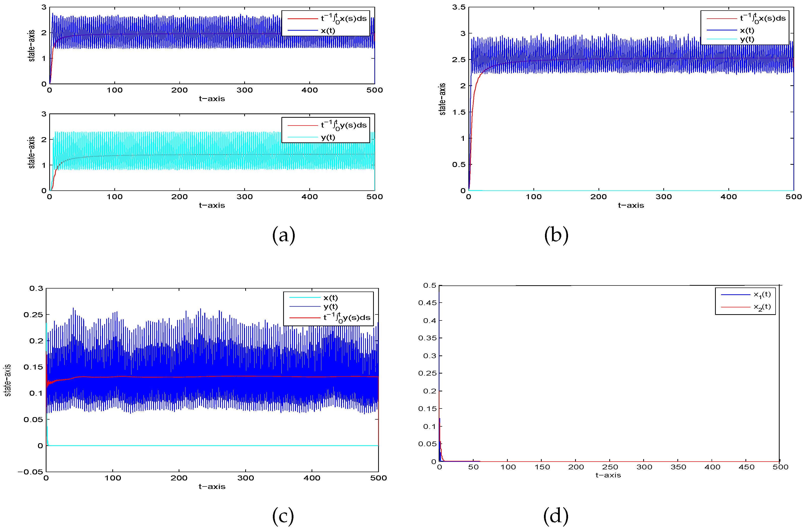
In this section, by applying the Milstein simulation method [30], we give some examples and simulations to illustrate our theoretical results and reveal the effects of random disturbance and impulsive factors.

Example 1.

In order to numerically examine the existence of a T-periodic solution of system (2), we choose the following parameters:

$$\begin{array}{ccc}{a}_{11}\left(t\right)=5+0.2sin2t,\hfill & a_{12}\left(t\right)=2+0.1cos2t,\hfill & c_1\left(t\right)=1+0.3cos2t,\hfill \\ m_0\left(t\right)=1+0.3sin2t,\hfill & m_1\left(t\right)=0.2+0.1sin2t,\hfill & m_2\left(t\right)=1+0.5sin2t,\hfill \\ a_{21}\left(t\right)=1+0.2sin2t,\hfill & a_{22}\left(t\right)=2+0.1sin2t,\hfill & c_2\left(t\right)=0.8+0.3cos2t,\hfill \\ {\sigma }_1\left(t\right)=0.02+0.02sin2t,\hfill & {\sigma }_2\left(t\right)=0.01+0.01sin2t,\hfill & {\xi }_1=0.03+0.01sin2t,\hfill \\ {\xi }_2=0.02+0.01sin2t,\hfill & t_k=k\pi ,k\in N,\hfill & \hfill \end{array}$$

such that (H${}_1$) holds. That is to say, the conditions of Theorem 2 are satisfied. By Theorem 2, we can see that system (2) has a unique π-periodic solution, illustrated in Figure 1a–c.

Figure 1. The periodic Markovian process for (2) with initial data $x_1\left(0\right)=x_2\left(0\right)=0.02.$ (a) The time series graph of $x_1\left(t\right)$ for Example 1; (b) the time series graph of $x_2\left(t\right)$ for Example 1; (c) the phase graph of Example 1 with ${\sigma }_i\left(t\right)\ne 0,{\xi }_{ik}\ne 0$; (d) the phase graph of deterministic system $({\xi }_{ik}={\sigma }_i\left(t\right)=0);$ (e) the phase graph of impulsive system $({\sigma }_i\left(t\right)=0,{\xi }_{ik}\ne 0)$; (f) the phase graph of stochastic system $({\sigma }_i\left(t\right)\ne 0,{\xi }_{ik}=0)i=1,2,k\in N$.

Furthermore, if there are no impulsive or stochastic effects, i.e., ${\sigma }_i\left(t\right)=0$ or ${\xi }_{ik}=0,$ other parameters remain unchanged, then by verification, (H${}_1$) holds and system (2) still has a $\pi$-periodic solution. The deterministic case (${\sigma }_i\left(t\right)={\xi }_{ik}=0$), the impulsive case (${\sigma }_i\left(t\right)=0$) and the stochastic case (${\xi }_{ik}=0$) are shown in Figure 1d–f, respectively.

By comparing (c) with (d–f), we can observe that small impulse or stochastic noise has little influence on the existence of the $\pi$-periodic solution.

Similarly, we can verify that all parameters meet (H${}_2$) and Theorem 3 shows that the solution of (2) is globally attractive. Figure 2 confirms this.

Figure 2. The attractivity of (2). The red lines are the time series of $x_1\left(t\right)$ and $x_2\left(t\right)$ with initial data $x_1\left(0\right)=x_2\left(0\right)=0.02$, and the blue lines are the time series of $x_1\left(t\right)$ and $x_2\left(t\right)$ with initial data $x_1\left(0\right)=x_2\left(0\right)=2.$ (a) The attractivity of $x_1\left(t\right)$; (b) The attractivity of $x_2\left(t\right)$.

Example 2.

We choose a set of parameters as follows in order to investigate the permanence and extinction of system (2). Let

$$\begin{array}{ccc}{a}_{11}\left(t\right)=2+0.2sin2t,\hfill & a_{12}\left(t\right)=0.8+0.1cos2t,\hfill & c_1\left(t\right)=0.5+0.3cos2t,\hfill \\ m_0\left(t\right)=0.5+0.3sin2t,\hfill & m_1\left(t\right)=0.2+0.1sin2t,\hfill & m_2\left(t\right)=0.8+0.5sin2t,\hfill \\ a_{21}\left(t\right)=0.6+0.2sin2t,\hfill & a_{22}\left(t\right)=0.4+0.1sin2t,\hfill & c_2\left(t\right)=1+0.3cos2t,\hfill \\ {\sigma }_1\left(t\right)=0.02+0.02sin2t,\hfill & {\sigma }_2\left(t\right)=0.01+0.01sin2t,\hfill & {\xi }_1=0.03+0.01sin2t,\hfill \\ {\xi }_2=0.02+0.01sin2t,\hfill & t_k=0.1k\pi ,k\in N.\hfill & \hfill \end{array}$$

It is not difficult to derive that ${\tilde{\lambda }}_1>0$ and ${\lambda }_2>0$. Then by Theorem 4, all species of (2) are permanent in the mean. Figure 3a confirms this.

Figure 3. The permanence in the mean and extinction of (2) with initial data $x_1\left(0\right)=x_2\left(0\right)=0.02.$ (a) the time series graph of $x_1\left(t\right)$ and $x_2\left(t\right)$; (b) the permanence in the mean of $x_1\left(t\right)$ and extinction of $x_2\left(t\right)$ with ${\sigma }_1\left(t\right)=0.02+0.02sin2t,{\sigma }_2\left(t\right)=2+0.01sin2t$; (c) the extinction of $x_1\left(t\right)$ and permanence in the mean of $x_2\left(t\right)$ with ${\xi }_1=2+0.01sin2t,{\xi }_2=1.8+0.01sin2t;$ (d) the extinction of all species with ${\sigma }_1\left(t\right)=2+0.02sin2t$ and ${\sigma }_2\left(t\right)=1+0.01sin2t$.

Next we illustrate the cases of extinction in Theorem 4. In order to reveal the impacts of stochastic or impulsive factors, we only change the values of stochastic or impulsive parameters and keep all other parameters the same.

(i)

Let ${\sigma }_2\left(t\right)=2+0.01sin2t$, then ${\tilde{\lambda }}_1>0$ and ${\tilde{\lambda }}_2<0$. Theorem 4 implies $x_1$ is permanent in the mean and $x_2$ is extinct, see Figure 3b. It shows that too much white noise results in the extinction of the predator.

(ii)

If ${\xi }_1=2+0.01sin2t,{\xi }_2=1.8+0.01sin2t,$ then ${\lambda }_1<0$ and ${\lambda }_2>0$. Theorem 4 implies $x_1$ is extinct and $x_2$ is permanent in the mean, as illustrated in Figure 3c, which shows that too large a pulse leads to the extinction of the prey.

(iii)

If ${\sigma }_1\left(t\right)=2+0.02sin2t,{\sigma }_2\left(t\right)=1+0.01sin2t$, then ${\lambda }_1<0$ and ${\tilde{\lambda }}_2<0$. Theorem 4 shows that both prey and predator are extinct (Figure 3d). This indicates that the white noise has a huge influence on the system permanence, and too much noise will make all species extinct.

Example 3.

For the autonomous and non-impulsive case, let $a_{11}=2, a_{12}=0.8, c_1=1, m_0=0.3$, $m_1=0.2, m_2=1, a_{21}=0.8, a_{22}=0.7, c_2=0.8, {\sigma }_1=0.2, {\sigma }_2=0.1.$ An easy computation shows that (H${}_3$) holds, so the distribution of (2) is stable (see Figure 4). Figure 4a,b shows the time series graphs of $x_1\left(t\right)$ and $x_2\left(t\right)$, respectively. Figure 4c is the density of distribution of $x_1\left(t\right)$ and $x_2\left(t\right)$.

Figure 4. The distribution of (13) with initial data $x_1\left(0\right)=x_2\left(0\right)=0.02.$ (a) the time series graph of $x_1\left(t\right)$; (b) the time series graph of $x_2\left(t\right)$; (c) the density of distribution of $x_1\left(t\right)$ and $x_2\left(t\right).$

7. Discussion and Conclusions

In this paper, a stochastic predator–prey system with impulsive effects and Beddington–DeAngelis functional responses is studied. The complicated dynamical behaviors are revealed in our main results. Sufficient conditions of the existence of periodic Markovian process are established in Theorem 2. The attractivity of solutions is shown in Theorem 3. The extinction and permanence in the mean of predator and prey species are represented in Theorem 4. The existence and ergodicity of the stationary distribution for the autonomous and non-impulsive cases of system (2) are given in Theorem 5. Finally, using Matlab, some simulations (Figure 1, Figure 2, Figure 3 and Figure 4) are given to verify the main results.

By giving some remarks (Remarks 1, 2 and 3), the main difference from some existing results are shown in detail. Particularly, we establish the sufficient conditions assuring the existence of a periodic Markovian process of (2), which has not been studied previously. In the process of our analysis, the Beddington–DeAngelis functional responses brought some difficulties and inequality techniques were applied to overcome them. When there are too many kinds of functional responses, what is the best way to deal with other functional responses? Further, time delays often appear in biological models; how should the effect of time delays be discussed? These are necessary and interesting questions for us to study in the future.

References

- Cantrell, R.S.; Cosner, C. On the dynamics of predator-prey models with the Bedding-DeAngelis functional response. J. Math. Anal. Appl. 2001, 257, 206–222. [Google Scholar] [CrossRef]
- Fan, M.; Kuang, Y. Dynamics of a non-autonomous predator-prey system with the Beddington-DeAngelis functional response. J. Math. Anal. Appl. 2004, 295, 15–39. [Google Scholar] [CrossRef] [Green Version]
- Wang, H. Global analysis of the predator-prey system with Beddington-DeAngelis functional response. J. Math. Anal. Appl. 2003, 281, 395–401. [Google Scholar] [CrossRef] [Green Version]
- Friedman, A. Stochastic Differential Equations and Their Applications; Academic Press: New York, NY, USA, 1976. [Google Scholar]
- Du, N.H.; Sam, V.H. Dynamics of a stochastic Lotka-Volterra model perturbed by white noise. J. Math. Anal. Appl. 2006, 324, 82–97. [Google Scholar] [CrossRef] [Green Version]
- Mao, X.; Marion, G.; Renshaw, E. Environmental Brownian noise suppresses explosions in populations dynamics. Stoch. Process. Appl. 2002, 97, 95–110. [Google Scholar] [CrossRef]
- Li, X.; Mao, X. Population dynamical behavior of non-autonomous Lotka-Volterra competitive system with random perturbation. Discret. Contin. Dyn. Syst. 2009, 24, 523–545. [Google Scholar] [CrossRef] [Green Version]
- Zuo, W.; Jiang, D.; Sun, X.; Hayat, T.; Alsaedib, A. Long-time behaviors of a stochastic cooperative Lotka-Volterra system with distributed delay. Physica A 2018, 506, 542–559. [Google Scholar] [CrossRef]
- Yagi, A.; Ton, T.V. Dynamic of a stochastic predator-prey population. Appl. Math. Comput. 2011, 218, 3100–3109. [Google Scholar] [CrossRef]
- Shao, Y.; Li, Y. Dynamical analysis of a stage structured predator-prey system with impulsive diffusion and generic functional response. Appl. Math. Comput. 2013, 220, 472–481. [Google Scholar] [CrossRef]
- Wu, R.H.; Zou, X.L.; Wang, K. Asymptotic behavior of a stochastic non-autonomous predator-prey model with impulsive perturbations. Commun. Nonlinear Sci. Numer. Simul. 2015, 20, 965–974. [Google Scholar] [CrossRef]
- Liu, M.; Wang, K. On a stochastic logistic equation with impulsive perturbations. Comput. Math. Appl. 2012, 63, 871–886. [Google Scholar] [CrossRef] [Green Version]
- Zhang, S.W.; Tan, D.J. Dynamics of a stochastic predator-prey system in a polluted environment with pulse toxicant input and impulsive perturbations. Appl. Math. Model. 2015, 39, 6319–6331. [Google Scholar] [CrossRef]
- Chen, L.J.; Chen, F.D. Dynamic behaviors of the periodic predator-prey system with distributed time delays and impulsive effect. Nonlinear Anal. Real World Appl. 2011, 12, 2467–2473. [Google Scholar] [CrossRef]
- Zhang, S.Q.; Meng, X.Z.; Feng, T.; Zhang, T.H. Dynamics analysis and numerical simulations of a stochastic non-autonomous predator-prey system with impulsive effects. Nonlinear Anal. Hybrid Syst. 2017, 26, 19–37. [Google Scholar] [CrossRef]
- Jiang, D.; Zuo, W.J.; Hayat, T.; Alsaedi, A. Stationary distribution and periodic solutions for stochastic Holling-Leslie predator-prey systems. Physica A 2016, 460, 16–28. [Google Scholar] [CrossRef]
- Zhao, Y.; Yuan, S.; Zhang, T.H. Stochastic periodic solution of a non-autonomous toxic-producing phytoplankton allelopathy model with environmental fluctuation. Commun. Nonlinear Sci. Numer. Simul. 2017, 44, 266–276. [Google Scholar] [CrossRef]
- Jiang, D.; Zhang, Q.M.; Hayat, T.; Alsaedi, A. Periodic solution for a stochastic non-autonomous competitive Lotka-Volterra model in a polluted environment. Physica A 2017, 471, 276–287. [Google Scholar] [CrossRef]
- Shao, Y. Globally asymptotical stability and periodicity for a nonautonomous two-species system with diffusion and impulses. Appl. Math. Model. 2012, 36, 288–300. [Google Scholar] [CrossRef]
- Li, D.; Xu, D. Periodic solutions of stochastic delay differential equations and applications to Logistic equation and neural networks. J. Korean Math. Soc. 2013, 50, 1165–1181. [Google Scholar] [CrossRef] [Green Version]
- Zhang, B.; Gopalsamy, K. On the periodic solution of N-dimensional stochastic population models. Stoch. Anal. Appl. 2000, 18, 323–331. [Google Scholar] [CrossRef]
- Zhang, Y.; Chen, S.H.; Gao, S.J.; Wei, X. Stochastic periodic solution for a perturbed non-autonomous predator-prey model with generalized nonlinear harvesting and impulses. Physica A 2017, 486, 347–366. [Google Scholar] [CrossRef]
- Zuo, W.J.; Jiang, D. Periodic solutions for a stochastic non-autonomous Holling-Tanner predator-prey system with impulses. Nonlin. Anal. Hybrid Syst. 2016, 22, 191–201. [Google Scholar] [CrossRef]
- Liu, M.; Wang, K. Asymptotic behavior of a stochastic nonautonomous Lotka-Volterra competitive system with impulsive perturbations. Math. Comput. Model. 2013, 57, 909–925. [Google Scholar] [CrossRef]
- Khas’minskii, R.Z. Stochastic Stability of Differential Equations; Sijthoff Noordhoff: Alphen aan den Rijn, The Netherlands; Springer Science & Business Media: Dordrecht, The Netherlands, 1980. [Google Scholar]
- Ji, C.Y.; Jiang, D. Dynamics of a stochastic density dependent predator-prey system with Beddington-DeAngelis functional response. J. Math. Anal. Appl. 2011, 381, 441–453. [Google Scholar] [CrossRef] [Green Version]
- Qiu, H.; Liu, M.; Wang, K.; Wang, Y. Dynamics of a stochastic predator-prey system with Beddington-DeAngelis functional response. Appl. Math. Comput. 2012, 219, 2303–2312. [Google Scholar] [CrossRef]
- Karatzas, I.; Shreve, S.E. Brownian Motion and Stochastic Calculus; Springer: Berlin/Heidelberg, Germany, 1991. [Google Scholar]
- Barbalat, I. Systems dequations differentielles d’osci d’oscillations nonlineaires. Rev. Roum. Math. Pures Appl. 1959, 4, 267–270. [Google Scholar]
- Higham, D.J. An algorithmic introduction to numerical simulation of stochastic differential equations. SIAM Rev. 2001, 43, 525–546. [Google Scholar] [CrossRef]
Publisher’s Note: MDPI stays neutral with regard to jurisdictional claims in published maps and institutional affiliations. |
© 2021 by the author. Licensee MDPI, Basel, Switzerland. This article is an open access article distributed under the terms and conditions of the Creative Commons Attribution (CC BY) license (https://creativecommons.org/licenses/by/4.0/).