Abstract
A fractional model of the Hopfield neural network is considered in the case of the application of the generalized proportional Caputo fractional derivative. The stability analysis of this model is used to show the reliability of the processed information. An equilibrium is defined, which is generally not a constant (different than the case of ordinary derivatives and Caputo-type fractional derivatives). We define the exponential stability and the Mittag–Leffler stability of the equilibrium. For this, we extend the second method of Lyapunov in the fractional-order case and establish a useful inequality for the generalized proportional Caputo fractional derivative of the quadratic Lyapunov function. Several sufficient conditions are presented to guarantee these types of stability. Finally, two numerical examples are presented to illustrate the effectiveness of our theoretical results.
1. Introduction
In [1], Jarad, Abdeljawad, and Alzabut introduced a new type of fractional derivative, the so-called generalized proportional fractional derivative. This type of derivative preserves the semigroup property, possesses a nonlocal character, and converges to the original function and its derivative upon limiting cases [2]. Some stability properties of the Ulam type for generalized proportional fractional differential equations were studied in [3] and in [4]. We emphasize that the regular stability has not been investigated yet. In this paper, we develop some necessary tools for the generalized Caputo proportional fractional derivatives, starting with an important inequality concerning an estimate of that derivative of quadratic functions. We derive some inequalities for quadratic Lyapunov functions and some connections between the solutions and the Lyapunov functions. These results are applied to study the stability properties of the Hopfield neural network with time-variable coefficients and Lipschitz activation functions. Due to its long-term memory, nonlocality, and weak singularity characteristics, fractional calculus has been successfully applied to various models of neural networks. For instance, Boroomand constructed the Hopfield neural networks based on fractional calculus [5], Kaslik analyzed the stability of Hopfield neural networks [6], Wang applied the fractional steepest descent algorithm to train BP neural networks and proved the monotonicity and convergence of a three-layer example [7]. The three features for the generalized proportional fractional derivative—the kernel of the fractional operator, the semi-group property of the generated fractional integrals, and obtaining the Riemann–Liouville and Caputo fractional derivatives as a special case—offers a possibility for more adequate modeling of some properties of the neural network.
The equilibrium of the studied model as well as its exponential stability and the Mittag–Leffler stability are defined and investigated.
The paper is organized as follows. In Section 2, some basic definitions and results are given. In Section 3, we present several auxiliary results for the generalized Caputo proportional fractional derivatives of the quadratic Lyapunov function. Section 4 contains the main results. The Hopfield neural model with time-variable coefficients and the generalized proportional fractional derivatives of the Caputo type are set up. The equilibrium is defined in an appropriate way. Exponential stability and Mittag–Leffler stability are defined, and several sufficient conditions are obtained. The paper concludes with Section 5, in which some detailed examples of neural networks are presented and simulated.
2. Preliminary Results
We recall that the generalized proportional fractional operators of a function ( are real numbers, and in the case of , the interval is open) are defined respectively by (see [2]):
- -
- the generalized proportional fractional integral
- -
- the generalized proportional Caputo fractional derivativewhere and are fixed parameters.
Remark 1.
The generalized proportional Caputo fractional derivative defined by (1) is a generalization of the Caputo fractional derivative (with ).
Remark 2.
Note that, in some works (for example, see [8,9,10]), the so-called tempered fractional integral and tempered fractional derivative are applied and defined by the following:
and
where is a fixed parameter. Tempered fractional integrals and tempered fractional derivatives are similar to the generalized proportional fractional integrals and derivatives (if , then and ).
Proposition 1
(Proposition 5.2, [1]). Let and . Then,
There is an explicit formula for the solution in the scalar linear case provided in Example 5.7 [1], which is (with an appropriate correction):
Proposition 2.
The solution of the linear Caputo proportional fractional initial value problem
is given by
where
are Mittag–Leffler functions with one parameter and two parameters, respectively.
3. Quadratic Lyapunov Functions and Their Generalized Proportional Derivatives
Initially, we will prove the following results for scalar functions:
Lemma 1.
Let the function with (if , then the interval is half open) and be two reals. Then,
Proof.
From definition (1), we have that for any ,
Use integration by parts and obtain the following:
The integral
has a singularity at the upper limit t, but it is a removable singularity because by the L’Hopital rule, we obtain the following:
Thus,
By the L’Hopital rule we get the following:
Inequality (8) proves the claim of Lemma 1. □
Inequality (4) is true in the vector case:
Corollary 1.
Let the function with (if , then the interval is half open) and . Then,
The proof follows from the decomposition of the scalar product into a sum of products and the application of Lemma 1.
Remark 3.
In the case of the Caputo fractional derivative, i.e., , the results of Lemma 1 and Corollary 1 are reduced to Lemma 1 [11] and Remark 1 [11].
Consider the following system of nonlinear fractional differential equations with the generalized proportional Caputo fractional derivative:
where , is the generalized proportional Caputo fractional derivative of the function , are two reals, and is a function.
Remark 4.
We will assume that for any initial value , the initial value problem (10) has a solution defined for .
Next, we will obtain two types of bounds for the solutions of (10).
Lemma 2.
Assume that:
- 1.
- The function is a solution of the IVP for the nonlinear system of generalized proportional Caputo fractional differential equations (10);
- 2.
- For any point , the inequalityholds.
Then,
Proof.
Define the function . Let be an arbitrary number. We will prove that
For , we get
i.e., inequality (13) is true for .
Now, assume that (13) is not true. Then there exist , such that
Denote . From (14), it follows that for . Therefore,
Thus, by the L’Hopital rule, we get the following:
From Proposition 1, inequality (17), and condition 2 for , we obtain the equation below:
The obtained contradiction proves the validity of (13) for any . Therefore,
i.e., the claim of Lemma 2 is true. □
Corollary 2.
Assume that the conditions of Lemma 2 are satisfied. Then, for all
The proof follows from inequality (12), , and the inequality .
Lemma 3.
Assume that:
- 1.
- The function is a solution of the IVP for the nonlinear system of generalized proportional Caputo fractional differential equations (10);
- 2.
- There exists a positive constant , such that at any point , the inequalityholds.
Then,
4. Stability of Neural Networks with a Generalized Proportional Caputo Fractional Derivative
The fractional-order Hopfield neural networks with the generalized proportional Caputo fractional derivative is described by the following equation:
where n is the number of units in a neural network, denotes the generalized proportional Caputo fractional derivative of order , is the state of the i-th unit at time t, denotes the activation function of the k-th neuron, denotes the connection weight of the k-th neuron on the i-th neuron at time t, represents the rate at which the i-th neuron resets its potential to the resting state when disconnected from the network at time t, and denotes the external inputs at time t.
We will now define the equilibrium of the neural network (23). Different than the classical case of ordinary derivatives and the Caputo fractional derivatives, in the general case, the equilibrium of (23) could not be a constant because the generalized proportional derivative of a nonzero constant is not 0. Applying Proposition 1, we define the equilibrium of (23):
Definition 1.
The function is called an equilibrium of (23) if
Remark 5.
The constant vector in Definition 1 could be a zero vector (zero equilibrium) or a nonzero vector (nonzero equilibrium).
Remark 6.
The zero vector is an equilibrium of (23) if and for all .
Let be an equilibrium of (23). Consider the change in the variables , in system (23), use Proposition 1 and obtain the following:
where , i.e., if is an equilibrium of (23), then the system
has a zero solution, and vice versa.
Definition 2.
Remark 7.
Note that the exponential stability is defined only for .
Remark 8.
The exponential stability of the equilibrium implies that every solution of (23) satisfies .
Definition 3.
Remark 9.
Note that the generalized Mittag–Leffler stability is defined for and for , and it generalizes the corresponding results for the Caputo fractional differential equations [6,12,13,14,15].
Remark 10.
Note that the Mittag–Leffler stability for the Hopfield neural network with tempered fractional derivatives is studied in [10,16], but only for zero equilibrium, zero internal perturbations, and constant coefficients.
Remark 11.
The generalized Mittag–Leffler stability of the equilibrium implies that every solution of (23) satisfies .
Theorem 1
(Exponential stability). Let the following assumptions hold:
- 1.
- and ;
- 2.
- The functions , ;
- 3.
- There exist positive constants , such that the activation functions satisfy for ;
- 4.
- Equation (23) has an equilibrium ;
- 5.
- The inequalityholds.
Then, the equilibrium of (23) is exponentially stable.
Proof.
Let be a solution of (23), and consider the system (25) with . From condition 3, we have the following equation:
for Then,
and by applying Condition 5, we get the following:
According to Lemma 2 applied to the system in (25), with , the inequality
holds. This proves the claim of the Theorem, with and . □
From Corollary 2 we obtain the following (applied to (23) with ):
Corollary 3
(Boundedness). Let , , and conditions 2–5 of Theorem 1 are satisfied. Then, any solution of (23) satisfies for all
Theorem 2
(Generalized Mittag–Leffler stability). Let the following assumptions hold:
- 1.
- Conditions 1–4 of Theorem 1 are satisfied;
- 2.
- There exists a positive constant L, such that inequalityholds.
Then, the equilibrium of (23) is Mittag–Leffler stable.
Proof.
Let be a solution of (23) and consider the system in (25) with . Similar to the proof of Theorem 1, we prove the following inequality:
Denote , and from (29) and Condition 2 of Theorem 2, it follows that there exists a function , such that
According to Proposition 2, the solution of the linear Caputo proportional fractional initial value problem (30) is given by the following equation:
From inequality (31), it follows that
□
5. Applications
Example 1.

Consider the following neural networks of neurons with a ring structure [6] with the following generalized proportional fractional derivatives:
where the activation functions are , i.e., condition 3 of Theorem 1 is satisfied by .
Case 1. Let be constants. Then, for , the system in (33) has no equilibrium because, for example, the following equality:
is not satisfied by any constant (compare with the case of the Caputo fractional derivative , [15]).
Case 2. Let . Then, for any , the system in (33) has zero equilibrium because (see Remark 6).
Case 3. Consider the following neural network:
Thus, the coefficients are as follows:
and
Then, for , the system in (33) has the equilibrium
because
hold.
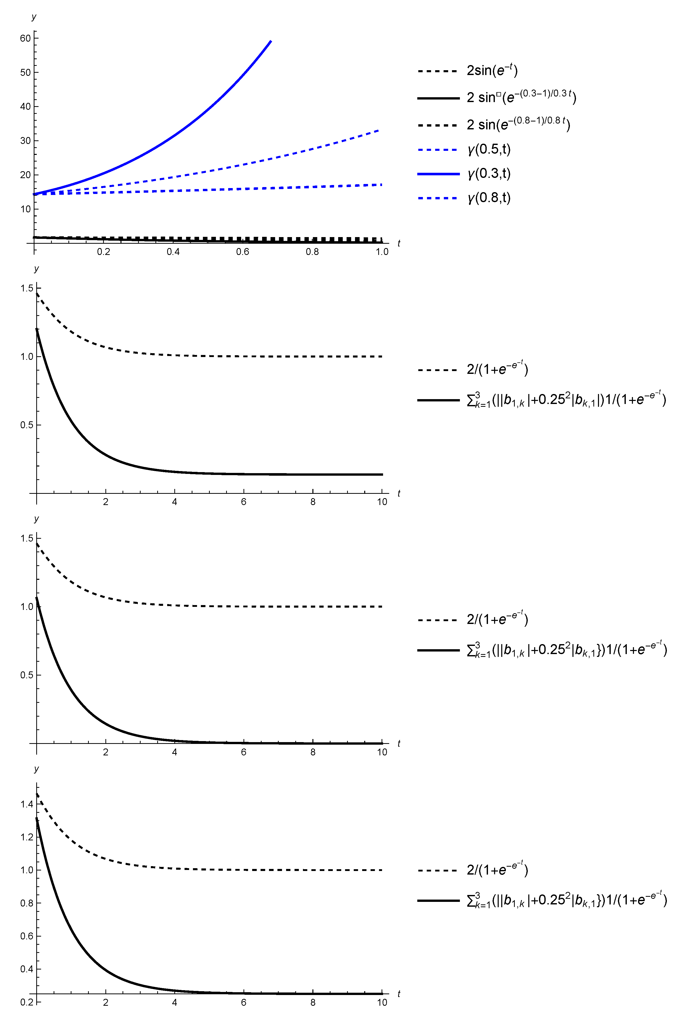
Neither the conditions of Theorem 1 nor the conditions of Theorem 2 are satisfied. For example, the following inequality:
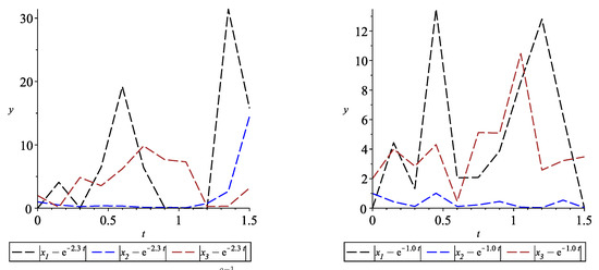
is not satisfied (see Figure 1, top left). Therefore, we are not able to conclude the stability properties of the equilibrium (see Figure 2).
Figure 2.
Graphs of functions , with and . On the (left), , and on the (right), .
Example 2.
Consider the following neural networks of neurons with the following generalized proportional fractional derivatives:
with the coefficients
the activation functions are equal to the sigmoid function, with , the perturbations are thus given by
and
Then, for , the system in (36) has the following equilibrium:
because
Moreover, condition 5 of Theorem 1 is satisfied because of the following inequalities:
(see Figure 1, top right, bottom left, and bottom right, respectively).
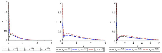
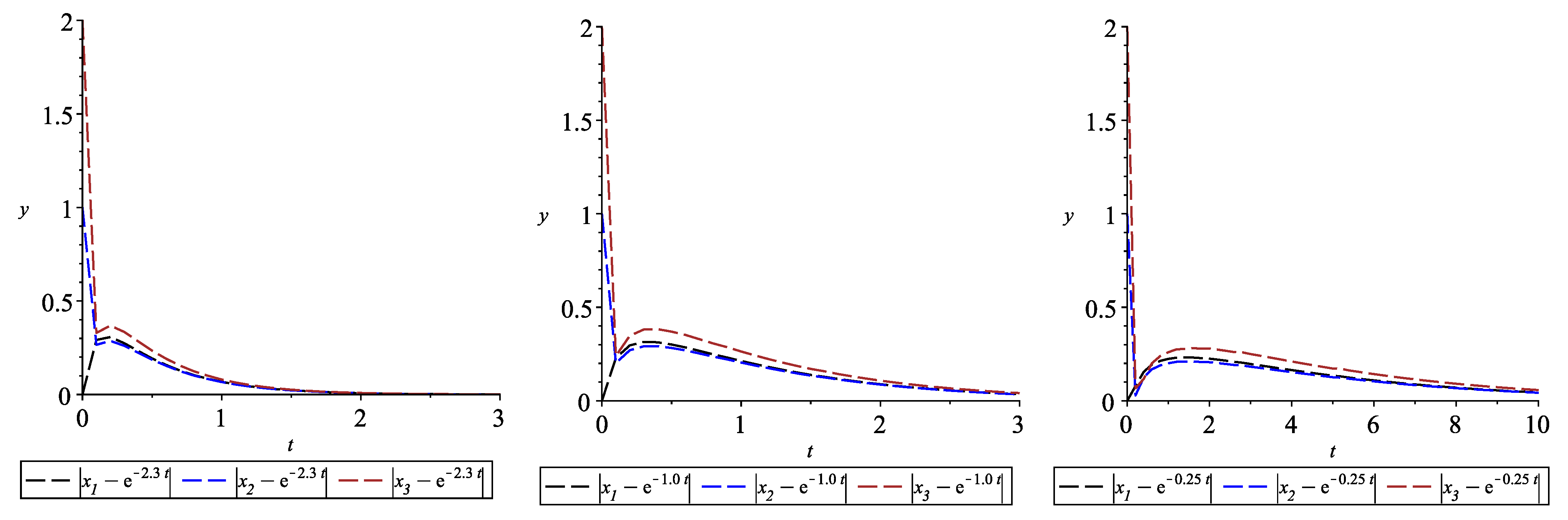
From Theorem 1, the equilibrium is exponentially stable, i.e., (see Figure 3)
Figure 3.
Graphs of the functions , with , , and (left), (center), and (right).
6. Conclusions
Initially, we proved an important inequality concerning an estimate of the generalized proportional Caputo fractional derivative of quadratic functions. The result could be applied to the study of various types of stability for the solutions of various types of fractional differential equations with the generalized proportional Caputo fractional derivative. In our paper, we applied it to study the stability properties of the Hopfiel neural network with the generalized proportional Caputo type fractional derivative. An equilibrium of the studied model was then defined. This equilibrium is generally not a constant (different than the case of ordinary derivatives and the Caputo type fractional derivatives). We defined the exponential stability and the Mittag–Leffler stability of the equilibrium. Several sufficient conditions were presented to guarantee these types of stability. The theoretical results were illustrated, with two numerical examples.
Author Contributions
Conceptualization, R.A., R.P.A., S.H. and D.O.; methodology, R.A., R.P.A., S.H. and D.O.; formal analysis, R.A., R.P.A., S.H. and D.O.; investigation, R.A., R.P.A., S.H. and D.O.; writing—original draft preparation, R.A., R.P.A., S.H. and D.O.; writing—review and editing, R.A., R.P.A., S.H. and D.O. All authors have read and agreed to the published version of the manuscript.
Funding
R.A. is supported by Portuguese funds through the CIDMA—Center for Research and Development in Mathematics and Applications, and the Portuguese Foundation for Science and Technology (FCT-Fundação para a Ciência e a Tecnologia), within project UIDB/04106/2020. S.H. is partially supported by the Bulgarian National Science Fund under Project KP-06-N32/7.
Conflicts of Interest
The authors declare no conflict of interest.
References
- Jarad, F.; Abdeljawad, T.; Alzabut, J. Generalized fractional derivatives generated by a class of local proportional derivatives. Eur. Phys. J. Spec. Top. 2017, 226, 3457–3471. [Google Scholar] [CrossRef]
- Alzabut, J.; Abdeljawad, T.; Jarad, F.; Sudsutad, W. A Gronwall inequality via the generalized proportional fractional derivative with applications. J. Ineq. Appl. 2019, 2019, 1–12. [Google Scholar] [CrossRef] [Green Version]
- Khaminsou, B.; Thaiprayoon, C.; Sudsutad, W.; Jose, S.A. Qualitative analysis of a proportional Caputo fractional differential pantograph differential equations with mixed nonlocal conditions. Nonl. Funct. Anal. Appl. 2021, 26, 197–223. [Google Scholar] [CrossRef]
- Sudsutad, W.; Alzabut, J.; Nontasawatsri, S.; Thaiprayoon, C. Stability analysis for a generalized proportional fractional Langevin equation with variable coefficient and mixed integro-differential boundary conditions. J. Nonlinear Funct. Anal. 2020, 2020, 1–24. [Google Scholar]
- Boroomand, A.; Menhaj, M.B. Fractional-Order Hopfield Neural Networks. In Advances in Neuro-Information Processing; 5506 of Lecture Notes in Computer Science; Springer: Berlin/Heidelberg, Germany, 2009; pp. 883–890. [Google Scholar]
- Kaslik, E.; Sivasundaram, S. Nonlinear dynamics and chaos in fractional-order neural networks. Neural Netw. 2012, 32, 245–256. [Google Scholar] [CrossRef] [PubMed]
- Wang, J.; Wen, Y.; Gou, Y.; Ye, Z.; Chen, H. Fractional-order gradient descent learning of BP neural networks with Caputo derivative. Neural Netw. 2017, 89, 19–30. [Google Scholar] [CrossRef] [PubMed]
- Deng, J.; Ma, W.; Deng, K.; Li, Y. Tempered Mittag—Leffler stability of tempered fractional dynamical systems. Math. Probl. Eng. 2020, 2020, 7962542. [Google Scholar] [CrossRef]
- Fernandez, A.; Ustaoglu, C. On some analytic properties of tempered fractional calculus. J. Comput. Appl. Math. 2020, 366, 112400. [Google Scholar] [CrossRef] [Green Version]
- Meerschaert, M.M.; Sabzikar, F.; Phanikumar, M.S.; Zeleke, A. Tempered fractional time series model for turbulence in geophysical flows. J. Stat. Mech. Theory Exper. 2014, 9, 9023. [Google Scholar] [CrossRef] [Green Version]
- Aguila–Camacho, N.; Duarte-Mermoud, M.A.; Gallegos, J.A. Lyapunov functions for fractional order systems. Commun. Nonlinear Sci. Numer. Simul. 2014, 19, 2951–2957. [Google Scholar] [CrossRef]
- Li, Y.; Chen, Y.Q.; Podlubny, I. Stability of fractional-order nonlinear dynamic systems: Lyapunov direct method and generalized Mittag—Leffler stability. Comput. Math. Appl. 2010, 59, 1810–1821. [Google Scholar] [CrossRef] [Green Version]
- Rajchakit, G.; Agarwal, P.; Ramalingam, S. Stability Analysis of Neural Networks; Springer: Singapore, 2021. [Google Scholar]
- Tanaka, K. Stability analysis of neural networks via Lyapunov approach. In Proceedings of the ICNN’95—International Conference on Neural Networks, Perth, WA, Australia, 27 November–1 December 1995. [Google Scholar] [CrossRef]
- Zhang, S.; Yu, Y.; Wang, H. Mittag–Leffler stability of fractional-order Hopfield neural networks. Nonlinear Anal. Hybrid Syst. 2015, 16, 104–121. [Google Scholar] [CrossRef]
- Gu, C.-Y.; Zheng, F.-H.; Shiri, B. Mittag–Leffler stability analysis of tempered fractional neural networks with short memory and variable-order. Fractals 2021, 8, 2140029. [Google Scholar] [CrossRef]

Publisher’s Note: MDPI stays neutral with regard to jurisdictional claims in published maps and institutional affiliations. |
© 2021 by the authors. Licensee MDPI, Basel, Switzerland. This article is an open access article distributed under the terms and conditions of the Creative Commons Attribution (CC BY) license (https://creativecommons.org/licenses/by/4.0/).