Local and Global Stability of Certain Mixed Monotone Fractional Second Order Difference Equation with Quadratic Terms

Abstract

This paper investigates the local and global character of the unique positive equilibrium of a mixed monotone fractional second-order difference equation with quadratic terms. The corresponding associated map of the equation decreases in the first variable, and it can be either decreasing or increasing in the second variable depending on the corresponding parametric values. We use the theory of monotone maps to study global dynamics. For local stability, we use the center manifold theory in the case of the non-hyperbolic equilibrium point. We show that the observed equation exhibits three types of global behavior characterized by the existence of the unique positive equilibrium, which can be locally stable, non-hyperbolic when there also exist infinitely many non-hyperbolic and stable minimal period-two solutions, and a saddle. Numerical simulations are carried out to better illustrate the results.

1. Introduction and Preliminaries

We consider difference equation:

$$x_{n+1}=\frac{B{x}_n{x}_{n-1}+F}{A{x}_n^2+b{x}_n{x}_{n-1}},n=0,1,\dots .$$

By substitution

$$x_n=\frac{B}{b}{y}_n$$

we get

$$y_{n+1}=\frac{\frac{B^3}{b}{y}_n{y}_{n-1}+bF}{\frac{A{B}^3}{b^2}{y}_n^2+\frac{B^3}{b}{y}_n{y}_{n-1}},n=0,1,\dots .$$

So, we consider the simpler equation:

$$x_{n+1}=\frac{x_n{x}_{n-1}+F}{A{x}_n^2+x_n{x}_{n-1}},n=0,1,\dots ,$$

(1)

where the parameters A, F are positive numbers and the initial conditions $x_0,x_{-1}$ are arbitrary non-negative real numbers such the denominator is defined.

We can note that Equation (1) is the special case of the following general second-order rational difference equation with quadratic terms

$$x_{n+1}=\frac{a{x}_n^2+b{x}_n{x}_{n-1}+c{x}_{n-1}^2+d{x}_n+e{x}_{n-1}+f}{A{x}_n^2+B{x}_n{x}_{n-1}+C{x}_{n-1}^2+D{x}_n+E{x}_{n-1}+F},n=0,1,\dots ,$$

where all of the parameters and the initial conditions are non-negative numbers such that: $a+b+c>0$, $A+B+C+D+E+F>0$, $n=0,1,\dots$, which has caught the attention of mathematical researchers over the last ten years. Over the past few decades, fractional-order systems have been considered for the modeling of realistic phenomena since they proved to be more practical to describe real-world processes compared to the classic integer-order models. It was demonstrated that the fractional models are capable of describing chaotic systems properly, so these models have appeared in different fields dealing with chaos, like mechanics, biology, and finance (see [1,2]). Additionally, these models were used for medical purposes such as for investigating the process of disease transmission and control, virus transmission, and to describe the performance of the human liver (see [3,4]).

The corresponding associated map of Equation (1) is always decreasing in the first variable and, it can be either decreasing or increasing in the second variable depending on the corresponding parametric values. The investigation of second-order difference equations with quadratic terms has intensified recently, and mostly equations whose monotonicity depends exclusively on the parameters have been examined. Due to the complexity, only a few authors deal with equations whose monotonicity depends on the initial conditions (see [5,6,7]).

We show that Equation (1) exhibits three types of global behavior characterized by the existence of the unique positive equilibrium, which is locally stable if $A<1$, non-hyperbolic if $A=1$ when there also exist infinitely many non-hyperbolic and stable minimal period-two solutions, and a saddle if $A>1$.

This paper is organized as follows. In Section 2, we investigate the existence of the equilibrium points and their local stability. Additionally, by center manifold theory (see [8]), we investigate the stability of the non-hyperbolic equilibrium point $\overline{x}.$ In Section 3, we investigate the existence of the minimal period-two solutions and their local stability. In Section 4, we give several global results obtained using the theory of monotone maps after we found an invariant and attracting interval on which the corresponding map does not change its monotonicity. The unique equilibrium point is global and asymptotically stable, in one case we have shown this by using the so-called “M-m theorem,” and for other cases, we used some techniques of mathematical analysis.

Through our paper we will use the following results:

Let I be some interval of real numbers and let $f\in C^1[I\times I,I]$. Let $\overline{x}\in I$, be an equilibrium point of a difference equation

$$x_{n+1}=f(x_n,x_{n-1}),x_{-1},x_0\in I,n=0,1,\dots ,$$

(2)

where f is continuous and decreasing in the first and increasing in the second variable. There are several global attractivity results for Equation (2) that give the sufficient conditions for all solutions to approach a unique equilibrium, such as:

Theorem 1.

(see [9]) Let $I=[a,b]$ be an interval of real numbers and assume that $f:I\times I\to I$ is a continuous function satisfying the following properties:

(a) 

$f(x,y)$ is non-increasing in the first and non-decreasing in the second variable.

(b) 

Equation (2) has no minimal period-two solutions in I.

Then every solution of Equation (2) converges to $\overline{x}$.

Theorem 2.

(see [10]) Let $I\subseteq \mathbb{R}$ be an interval and let $f\in C[I\times I,I]$ be a function that is non-increasing in the first and non-decreasing in the second variable. Then for every solution of Equation (2) the subsequences ${\left\{x_{2n}\right\}}_{n=0}^{\infty }$ and ${\left\{x_{2n+1}\right\}}_{n=-1}^{\infty }$ of even and odd terms of the solution do exactly one of the following:

(i) 

Eventually, they are both monotonically increasing.

(ii) 

Eventually, they are both monotonically decreasing.

(iii) 

One of them is monotonically increasing, and the other is monotonically decreasing.

We will use the following result from [11].

Theorem 3.

Let $[a,b]$ be a compact interval of real numbers and assume that $f:[a,b]\times [a,b]\to [a,b]$ is a continuous function satisfying the following properties:

(a) 

$f(x,y)$ is non-increasing in both variables in $[a,b]$;

(b) 

If $(m,M)\in [a,b]\times [a,b]$ is a solution of the system

$$f(m,m)=M\mathrm{and}f(M,M)=m,$$

(3)

then $m=M$.

Then

$$x_{n+1}=f(x_n,x_{n-1}),n=0,1,\dots$$

(4)

has a unique equilibrium $\overline{x}\in [a,b]$, and every solution of Equation (4) converges to $\overline{x}$.

The following result is also the global attractivity result in [9,12] for monotone maps that we will use here.

Theorem 4.

Assume that the difference equation

$$x_{n+1}=G\left(x_n,\dots ,x_{n-k}\right),n=0,1,\dots ,$$

where G is non-decreasing functions in all its arguments has the unique equilibrium $\overline{x}\in I$, where I is an invariant interval, i.e., $G:I^{k+1}\to I$. Then $\overline{x}$ is globally asymptotically stable.

To obtain the convergence results, we will also use the following Lemma ([13], Theorem 1.8).

Lemma 1.

Consider the difference equation

$$x_{n+1}=f(x_n,x_{n-1},\dots ,x_{n-k})$$

(5)

where $f\in C[J^{k+1},J]$ for some interval J of real numbers and some non-negative integer k. Let ${\left\{x_n\right\}}_{n=-k}^{\infty }$ be a solution of (5). Set ${\displaystyle I=\underset{n\to \infty }{lim\; inf}{x}_n}$ and ${\displaystyle S=\underset{n\to \infty }{lim\; sup}{x}_n}$, and suppose that I, $S\in J$. Let ${\mathcal{L}}_0$ be a limit point of the sequence ${\left\{x_n\right\}}_{n=-k}^{\infty }$. Then the following statements are true.

1. 

There exists a solution ${\left\{L_n\right\}}_{n=-\infty }^{\infty }$ of (5), called a full limiting sequence of ${\left\{x_n\right\}}_{n=-k}^{\infty }$, such that $L_0={\mathcal{L}}_0$, and such that for every $N\in \mathbb{Z}$, $L_N$ is a limit point of ${\left\{x_n\right\}}_{n=-k}^{\infty }$. In particular

$$I\le L_n\le SforallN\in \mathbb{Z}.$$

2. 

For every $i_0\in \mathbb{Z}$, there exists a subsequence ${\left\{x_{r_i}\right\}}_{i=0}^{\infty }$ of the solution ${\left\{x_n\right\}}_{n=-k}^{\infty }$ such that

$$L_N=\underset{i\to \infty }{lim}{x}_{r_i+N}foreveryN\ge i_0.$$

2. The Equilibrium Point and Linearized Stability

This section proves that Equation (1) has a unique positive equilibrium that can be locally asymptotically stable, non-hyperbolic, or a saddle point in a particular parametric space.

Equation (1) has the unique positive equilibrium point $\overline{x}$, which is the positive root of the equation

$$\phi \left(x\right)=\left(A+1\right)x^3-x^2-F=0.$$

The equation $\phi \left(x\right)=0$ has only one real solution and two conjugate-complex solutions. Notice that $\phi \left(0\right)=-F<0$. The function $\phi$ has a local maximum at $x=0$ and a local minimum at $x=\frac{2}{3\left(A+1\right)}>0$ with $\phi \left(\frac{2}{3\left(A+1\right)}\right)=-F-\frac{4}{27{\left(A+1\right)}^2}<0$. It means that function $\phi$ has only one positive root, i.e., Equation (1) has a unique positive equilibrium point.

Denote

$$f\left(u,v\right)=\frac{uv+F}{A{u}^2+uv}.$$

A linearization of (1) is of the form

$$r_{n+1}=s{r}_n+t{r}_{n-1},$$

(6)

where

$$\begin{array}{ccc}\hfill s& =& {\frac{\partial f\left(u,v\right)}{\partial u}}_{\left(u,v\right)=\left(\overline{x},\overline{x}\right)}=-\frac{A{\overline{x}}^2+\left(2A+1\right)F}{{\overline{x}}^3{\left(A+1\right)}^2}=\frac{1-\left(2A+1\right)\overline{x}}{\overline{x}\left(A+1\right)},\hfill \\ \hfill t& =& {\frac{\partial f\left(u,v\right)}{\partial v}}_{\left(u,v\right)=\left(\overline{x},\overline{x}\right)}=\frac{A{\overline{x}}^2-F}{{\overline{x}}^3{\left(A+1\right)}^2}=\frac{1-\overline{x}}{\left(A+1\right)\overline{x}}.\hfill \end{array}$$

In the expressions for s and t we used relation $F=\left(A+1\right){\overline{x}}^3-{\overline{x}}^2$ which follows from $\phi \left(\overline{x}\right)=0$.

We can see that $\left|t\right|<1$ and $s<0$. Namely,

$$\left|t\right|<1⟺\left(-1<\frac{1-\overline{x}}{\left(A+1\right)\overline{x}}<1\right)⟺\left(-A\overline{x}<1\mathrm{and}\overline{x}>\frac{1}{A+2}\right)$$

which is true because $0<F=\left(\left(A+1\right)\overline{x}-1\right){\overline{x}}^2⟹\left(A+1\right)\overline{x}-1>0$ i.e., $\overline{x}>\frac{1}{A+1}>\frac{1}{A+2}$ and A, $\overline{x}$ are positive. Thus, the equilibrium is non-hyperbolic if it is satisfied $-s=1-t$. We get

$$-s=1-t⟺\frac{\left(2A+1\right)\overline{x}-1}{\overline{x}\left(A+1\right)}=1-\frac{1-\overline{x}}{\left(A+1\right)\overline{x}}⟺\frac{2A\overline{x}}{\overline{x}\left(A+1\right)}=1⟺A=1.$$

If $A=1$, then $s=\frac{1-3\overline{x}}{2\overline{x}}$ and $t=\frac{1-\overline{x}}{2\overline{x}}$, so the characteristic equation of (6) has eigenvalues:

$${\lambda }_{\pm }=\frac{s\pm \sqrt{s^2+4t}}{2}=\frac{1}{4}\left(\frac{1-3\overline{x}}{\overline{x}}\pm \frac{\overline{x}+1}{\overline{x}}\right),$$

i.e., ${\lambda }_{-}=-1$, ${\lambda }_{+}=-\frac{\overline{x}-1}{2\overline{x}}$. From $x>\frac{1}{A+1}=\frac{1}{2}$ follows ${\lambda }_{+}=\frac{1-\overline{x}}{2\overline{x}}=\frac{1}{2\overline{x}}-\frac{1}{2}<1-\frac{1}{2}=\frac{1}{2}$. Notice ${\lambda }_{+}>-1\iff \frac{1-\overline{x}}{2\overline{x}}>-1\iff 1-\overline{x}>-2\overline{x}\iff \overline{x}>-1$, which is true. Similarly we conclude that

$$\begin{array}{c}{\lambda }_{+}\in \left(-1,0\right)⟺\overline{x}>1⟹0=\phi \left(\overline{x}\right)={\overline{x}}^2\left(2\overline{x}-1\right)-F>1-F,\mathrm{i.e.},F>1,\hfill \\ {\lambda }_{+}=0⟺\overline{x}=1⟹0=\phi \left(\overline{x}\right)={\overline{x}}^2\left(2\overline{x}-1\right)-F=1-F,\mathrm{i.e.},F=1,\hfill \\ {\lambda }_{+}\in \left(0,\frac{1}{2}\right)⟺\frac{1}{2}<\overline{x}<1⟹0=\phi \left(\overline{x}\right)={\overline{x}}^2\left(2\overline{x}-1\right)-F<1-F,\mathrm{i.e.},F<1.\hfill \end{array}$$

The equilibrium point $\overline{x}$ is locally asymptotically stable if the condition

$$-s<1-t$$

is satisfied so, we have

$$\begin{array}{cc}-s<1-t\hfill & ⟺\frac{1-\left(2A+1\right)\overline{x}}{\overline{x}\left(A+1\right)}-\frac{1-\overline{x}}{\left(A+1\right)\overline{x}}+1>0⟺A<1.\hfill \end{array}$$

The equilibrium point $\overline{x}$ is a saddle point if it holds $-s<1-t⟺A>1$. We proved the next theorem:

Theorem 5.

The unique equilibrium point $\overline{x}$ of Equation (1) is

(i) 

locally asymptotically stable (LAS) if $A<1$,

(ii) 

a saddle point (SP) if $A>1$,

(iii) 

a non-hyperbolic (NH) if $A=1$, with eigenvalues

$${\lambda }_{-}=-1,{\lambda }_{+}=-\frac{\overline{x}-1}{2\overline{x}}$$

and we have

$$\begin{array}{c}\hfill {\lambda }_{+}\in \left(-1,0\right)⟺F>1\left(\overline{x}>1\right),\\ \hfill {\lambda }_{+}=0⟺F=1\left(\overline{x}=1\right),\\ \hfill {\lambda }_{+}\in \left(0,\frac{1}{2}\right)⟺F<1\left(\frac{1}{2}<\overline{x}<1\right).\end{array}$$

In the following analysis, we investigate the stability of the non-hyperbolic equilibrium point $\overline{x}.$

Theorem 6.

Assume that $A=1$. Then the positive equilibrium point $\overline{x}$ of Equation (1) is unstable.

Proof. 

To prove that $\overline{x}$ is unstable we will use center manifold theory. Equation (1) is of the form

$$x_{n+1}=\frac{x_n{x}_{n-1}+F}{x_n^2+x_n{x}_{n-1}}$$

(7)

By the change of variable $y_n=x_n-\overline{x}$, for $F=2{\overline{x}}^3-{\overline{x}}^2$ we obtain the following equation

$$y_{n+1}=\frac{y_n{y}_{n-1}+\overline{x}{y}_n-{\overline{x}}^2{y}_{n-1}-\overline{x}{y}_n^2-3{\overline{x}}^2{y}_n+\overline{x}{y}_{n-1}-\overline{x}{y}_n{y}_{n-1}}{\left(\overline{x}+y_n\right)\left(2\overline{x}+y_n+y_{n-1}\right)}$$

(8)

which has a zero equilibrium. By the substitution $y_{n-1}=u_n,y_n=v_n$, Equation (1) becomes the system

$$\left.\begin{array}{c}{u}_{n+1}=v_n\hfill \\ v_{n+1}=\frac{v_n{u}_n+\overline{x}{v}_n-{\overline{x}}^2{u}_n-\overline{x}{v}_n^2-3{\overline{x}}^2{v}_n+\overline{x}{u}_n-\overline{x}{v}_n{u}_n}{\left(\overline{x}+v_n\right)\left(2\overline{x}+v_n+u_n\right)}\hfill \end{array}\right\}.$$

(9)

The Jacobian matrix $J_0$ at the zero equilibrium for (9) is

$$J_0=\left[\begin{array}{cc}0& 1\\ \frac{1-\overline{x}}{2\overline{x}}& \frac{1-3\overline{x}}{2\overline{x}}\end{array}\right]$$

and the corresponding characteristic equation has the form

$${\lambda }^2-\frac{1-3}{2\overline{x}}\lambda -\frac{1-\overline{x}}{2\overline{x}}=0,$$

with

$${\lambda }_1=-1,{\lambda }_2=\frac{1-\overline{x}}{2\overline{x}}.$$

Now, the initial system can be written as

$$\left[\begin{array}{c}{u}_{n+1}\\ v_{n+1}\end{array}\right]=J_0\left[\begin{array}{c}{u}_n\\ v_n\end{array}\right]+\left[\begin{array}{c}\gamma \left(u_n,v_n\right)\\ \zeta \left(u_n,v_n\right)\end{array}\right]$$

(10)

where

$$\begin{array}{cc}\hfill \gamma \left(u,v\right)& =0,\hfill \\ \hfill \zeta \left(u,v\right)& =\frac{vu+\overline{x}v-{\overline{x}}^{2}u-\overline{x}{v}^2-3{\overline{x}}^{2}v+\overline{x}u-\overline{x}vu}{\left(\overline{x}+v\right)\left(2\overline{x}+v+u\right)}-\frac{1-\overline{x}}{2\overline{x}}u-\frac{1-3\overline{x}}{2\overline{x}}v,\hfill \end{array}$$

i.e.,

$$\left.\begin{array}{c}\gamma \left(u,v\right)=0\hfill \\ \zeta \left(u,v\right)=\frac{-2u{v}^2-u^{2}v-u^2\overline{x}-3v^2\overline{x}+3v^3\overline{x}+u^2{\overline{x}}^2+7v^2{\overline{x}}^2-v^3+4uv{\overline{x}}^2+4u{v}^2\overline{x}+u^{2}v\overline{x}-2uv\overline{x}}{2\overline{x}\left(v+\overline{x}\right)\left(u+v+2\overline{x}\right)}\hfill \end{array}\right\}$$

(11)

We let now

$$\left[\begin{array}{c}{u}_n\\ v_n\end{array}\right]=P\left[\begin{array}{c}{r}_n\\ s_n\end{array}\right]$$

(12)

where P is the matrix that diagonalizes $J_0$ defined by

$$P=\left[\begin{array}{cc}\hfill 1& 1\\ \hfill -1& \frac{1-\overline{x}}{2\overline{x}}\end{array}\right],$$

such that

$$P^{-1}=\frac{2\overline{x}}{\overline{x}+1}\left[\begin{array}{cc}\frac{1-\overline{x}}{2\overline{x}}& \hfill -1\\ 1& \hfill 1\end{array}\right],$$

and

$$P^{-1}{J}_{0}P=\left[\begin{array}{cc}\hfill -1& 0\\ \hfill 0& \frac{1-\overline{x}}{2\overline{x}}\end{array}\right].$$

(13)

By (12) we have

$$\begin{array}{cc}\hfill u_n& =r_n+s_n,\hfill \\ \hfill v_n& =-r_n+\frac{1-\overline{x}}{2\overline{x}}{s}_n,\hfill \end{array}$$

and by substitution in (11) we have

$$\begin{array}{cc}\hfill \gamma \left(u_n,v_n\right)& =\overline{\gamma }\left(r_n,s_n\right),\hfill \\ \hfill \zeta \left(u_n,v_n\right)& =\overline{\zeta }\left(r_n,s_n\right),\hfill \end{array}$$

i.e.,

$$\begin{array}{cc}\hfill \overline{\gamma }\left(r_n,s_n\right)& =0,\hfill \\ \hfill \overline{\zeta }\left(r_n,s_n\right)& =\frac{8r_n^2{\overline{x}}^3\left(-2\overline{x}+s_n+\overline{x}{s}_n+4{\overline{x}}^2\right)+2r_n\overline{x}{s}_n\left(3\overline{x}-1\right)\left(-s_n+{\overline{x}}^2{s}_n-8{\overline{x}}^2+4{\overline{x}}^3\right)+s_n^2{\left(\overline{x}-1\right)}^3\left(s_n+\overline{x}{s}_n+6{\overline{x}}^2\right)}{4{\overline{x}}^2\left(-2\overline{x}{r}_n+\left(1-\overline{x}\right)s_n+2{\overline{x}}^2\right)\left(\left(1+\overline{x}\right)s_n+4{\overline{x}}^2\right)}.\hfill \end{array}$$

Thus, (10) can be written as

$$P\left[\begin{array}{c}{r}_{n+1}\\ s_{n+1}\end{array}\right]=J_{0}P\left[\begin{array}{c}{r}_n\\ s_n\end{array}\right]+\left[\begin{array}{c}\overline{\gamma }\left(r_n,s_n\right)\\ \overline{\zeta }\left(r_n,s_n\right)\end{array}\right]$$

or equivalently

$$\left[\begin{array}{c}{r}_{n+1}\\ s_{n+1}\end{array}\right]=P^{-1}{J}_{0}P\left[\begin{array}{c}{r}_n\\ s_n\end{array}\right]+P^{-1}\left[\begin{array}{c}\overline{\gamma }\left(r_n,s_n\right)\\ \overline{\zeta }\left(r_n,s_n\right)\end{array}\right].$$

Using (13) we have

$$\left[\begin{array}{c}{r}_{n+1}\\ s_{n+1}\end{array}\right]=\left[\begin{array}{cc}\hfill -1& 0\\ \hfill 0& \frac{1-\overline{x}}{2\overline{x}}\end{array}\right]\left[\begin{array}{c}{r}_n\\ s_n\end{array}\right]+P^{-1}\left[\begin{array}{c}\overline{\gamma }\left(r_n,s_n\right)\\ \overline{\zeta }\left(r_n,s_n\right)\end{array}\right].$$

(14)

So the normal form of System (10) is of the form

$$\left[\begin{array}{c}{r}_{n+1}\\ s_{n+1}\end{array}\right]=\left[\begin{array}{cc}\hfill -1& 0\\ \hfill 0& \frac{1-\overline{x}}{2\overline{x}}\end{array}\right]\left[\begin{array}{c}{r}_n\\ s_n\end{array}\right]+\left[\begin{array}{c}\widehat{\gamma }\left(r_n,s_n\right)\\ \widehat{\zeta }\left(r_n,s_n\right)\end{array}\right],$$

where

$$\widehat{\gamma }\left(r_n,s_n\right)=-\widehat{\zeta }\left(r_n,s_n\right),$$

and

$$\widehat{\gamma }\left(r_n,s_n\right)=-\frac{8r_n^2{\overline{x}}^3\left(\left(1+\overline{x}\right)s_n+2\overline{x}\left(2\overline{x}-1\right)\right)+2r_n\overline{x}{s}_n\left(3\overline{x}-1\right)\left(\left({\overline{x}}^2-1\right)s_n+4{\overline{x}}^2\left(\overline{x}-2\right)\right)+s_n^2{\left(\overline{x}-1\right)}^3\left(\left(1+\overline{x}\right)s_n+6{\overline{x}}^2\right)}{2\overline{x}\left(\overline{x}+1\right)\left(4{\overline{x}}^2+s_n\left(\overline{x}+1\right)\right)\left(\left(1-\overline{x}\right)s_n-2\overline{x}{r}_n+2{\overline{x}}^2\right)}.$$

We now let

$$s=\chi \left(r\right)=\Psi \left(r\right)+O\left(r^4\right),$$

where

$$\Psi \left(r\right)=\alpha r^2+\beta r^3,\alpha ,\beta \in \mathbb{R}$$

is the center manifold, and where map $\chi$ must satisfy the center manifold equation (for ${\lambda }_2=\frac{1-\overline{x}}{2\overline{x}}$)

$$\chi \left(-r+\widehat{\gamma }\left(r,\chi \left(r\right)\right)\right)-{\lambda }_2\chi \left(r\right)-\widehat{\zeta }\left(r,\chi \left(r\right)\right)=0.$$

(15)

If we approximate $\widehat{\gamma }(r,s$) by a Taylor polynomial as follows

$$\widehat{\gamma }\left(r,s\right)=\sum _{i=1}^3\frac{1}{i!}{\left(r\frac{\partial }{\partial r}y(0,0)+s\frac{\partial }{\partial s}y(0,0)\right)}^i+O_4,$$

we obtain

$$\widehat{\gamma }\left(r,\chi \left(r\right)\right)=-\frac{1}{2\overline{x}\left(\overline{x}+1\right)}\left(\frac{3\alpha {\overline{x}}^2-\left(7\alpha -4\right)\overline{x}+2\left(\alpha -1\right)}{2{\overline{x}}^2\left(\overline{x}+1\right)}{r}^3+\frac{\left(2\overline{x}-1\right)}{\overline{x}\left(\overline{x}+1\right)}{r}^2\right)+O\left(r^4\right)$$

and

$$\chi \left(-r+\widehat{\gamma }\left(r,\chi \left(r\right)\right)\right)=\frac{-\left(\alpha -2\overline{x}\alpha +{\overline{x}}^2\beta +2{\overline{x}}^3\beta +{\overline{x}}^4\beta \right)r^3+{\overline{x}}^2\alpha {\left(\overline{x}+1\right)}^2{r}^2}{{\overline{x}}^2{\left(\overline{x}+1\right)}^2}+O\left(r^4\right).$$

From (15) we have the following system

$$\begin{array}{cc}\hfill \left(\overline{x}+1\right)\left(5\overline{x}-2\right)\alpha -2{\overline{x}}^2{\left(\overline{x}+1\right)}^3\beta & =2\left(2\overline{x}-1\right)\hfill \\ \hfill \alpha \overline{x}\left(3\overline{x}-1\right){\left(\overline{x}+1\right)}^2& =2\overline{x}-1\hfill \end{array}$$

whose solution is $\left(\alpha ,\beta \right)=\left(\frac{2\overline{x}-1}{\overline{x}\left(3\overline{x}-1\right){\left(\overline{x}+1\right)}^2},\frac{-\left(2\overline{x}-1\right)\left(6{\overline{x}}^3+4{\overline{x}}^2-7\overline{x}+2\right)}{2{\overline{x}}^3{\left(\overline{x}+1\right)}^4\left(3\overline{x}-1\right)}\right)$.

Let $s=\chi \left(r\right)=\Psi \left(r\right)+O\left(r^4\right)$, where

$$\Psi \left(r\right)=\frac{2\overline{x}-1}{\overline{x}\left(3\overline{x}-1\right){\left(\overline{x}+1\right)}^2}{r}^2-\frac{\left(2\overline{x}-1\right)\left(6{\overline{x}}^3+4{\overline{x}}^2-7\overline{x}+2\right)}{2{\overline{x}}^3{\left(\overline{x}+1\right)}^4\left(3\overline{x}-1\right)}{r}^3.$$

In view of Theorem 5.9 of [14] the study of the stability of the zero equilibrium of Equation (8), that is the positive non-hyperbolic equilibrium of Equation (7), reduces to the stability of the following equation

$$r_{n+1}=-r_n+\widehat{\gamma }\left(r_n,s_n\right)=G\left(r_n\right),$$

(16)

where

$$G\left(r\right)=-r+\widehat{\gamma }\left(r,\Psi \left(r\right)\right)=-r-\frac{2\overline{x}-1}{2{\overline{x}}^2{\left(\overline{x}+1\right)}^2}\left(\frac{2{\overline{x}}^3+4{\overline{x}}^2+3\overline{x}-2}{2{\overline{x}}^2{\left(\overline{x}+1\right)}^2}{r}^3+r^2\right).$$

Since

$$\begin{array}{ccc}\hfill \frac{d\left(G\left(0\right)\right)}{dr}& =& -1,\hfill \\ \hfill \frac{d^2\left(G\left(0\right)\right)}{d{r}^2}& =& -\frac{2\overline{x}-1}{{\overline{x}}^2{\left(\overline{x}+1\right)}^2},\hfill \\ \hfill \frac{d^3\left(G\left(0\right)\right)}{d{r}^3}& =& -\frac{3\left(2\overline{x}-1\right)\left(2{\overline{x}}^3+4{\overline{x}}^2+3x-2\right)}{2{\overline{x}}^4{\left(\overline{x}+1\right)}^4},\hfill \end{array}$$

then the corresponding Schwarzian is of the form

$$\begin{array}{cc}\hfill S_{G\left(0\right)}& =-\frac{d^3\left(G\left(0\right)\right)}{d{r}^3}-\frac{3}{2}{\left(\frac{d^2\left(G\left(0\right)\right)}{d{r}^2}\right)}^2\hfill \\ \hfill & =-\left(-\frac{3\left(2\overline{x}-1\right)\left(2{\overline{x}}^3+4{\overline{x}}^2+3\overline{x}-2\right)}{2{\overline{x}}^4{\left(\overline{x}+1\right)}^4}\right)-\frac{3}{2}{\left(\frac{1-2\overline{x}}{{\overline{x}}^2{\left(\overline{x}+1\right)}^2}\right)}^2\hfill \\ \hfill & =\frac{3\left(2\overline{x}-1\right)\left(2{\overline{x}}^2+2\overline{x}-1\right)}{2{\overline{x}}^4{\left(\overline{x}+1\right)}^3}>0,\mathrm{since}\overline{x}>\frac{1}{2},\hfill \end{array}$$

and from Theorem 1.6 of [11], the zero equilibrium of (16) is unstable. Therefore, from Theorem 5.9 of [14], the zero equilibrium of Equation (8), that is the positive non-hyperbolic equilibrium of Equation (7) is unstable. □

3. The Minimal Period-Two Solutions

Now we present results about the existence and stability of minimal period-two solutions of Equation (1).

Lemma 2.

If $A=1$, then Equation (1) has infinitely many minimal period-two solutions

$$\{\dots ,\psi ,\varphi ,\psi ,\varphi ,\dots \}\left(\varphi \ne \psi \mathrm{and}\varphi >0\mathrm{and}\psi >0\right)$$

(17)

such that

$$\psi {\varphi }^2+({\psi }^2-\psi )\varphi -F=0.$$

(18)

Proof. 

Suppose that there exists a minimal period-two solution $\{\dots ,\varphi ,\psi ,\varphi ,\psi ,\dots \}$ of Equation (1), where $\varphi$ and $\psi$ are distinct non-negative real numbers. Then we have the following system:

$$\left.\begin{array}{c}\varphi =\frac{\psi \varphi +F}{A{\psi }^2+\psi \varphi }\\ \psi =\frac{\varphi \psi +F}{A{\varphi }^2+\varphi \psi }\end{array}\right\}\iff$$

$$\left.\begin{array}{c}A\varphi {\psi }^2+{\varphi }^2\psi =\varphi \psi +F\\ A{\varphi }^2\psi +\varphi {\psi }^2=\varphi \psi +F\end{array}\right\}.$$

(19)

It has to be $\varphi \ne 0$ and $\psi \ne 0$. By subtracting equations of the system (19) we get the following

$$\begin{array}{c}\varphi \psi \left(A\right(\psi -\varphi )-(\psi -\varphi \left)\right)=0,\\ \varphi \psi (\psi -\varphi )(A-1)=0.\end{array}$$

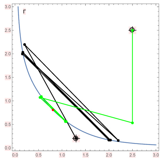
For $A=1$, we have only one equation, which is the Equation (18). We conclude that Equation (1) has infinitely many period two solutions of the form $(\varphi ,\psi )$, where $\varphi$ and $\psi$ are arbitrary positive numbers which satisfy Equation (18), i.e., that lie on the curve $\Gamma$ shown in the Figure 1. □

Figure 1. Visualization of Conjecture 3 with $A=1$, $F=0.4$ and initial conditions $(x_{-1},x_0)=(1.3,0.2)$—black, $(x_{-1},x_0)=(2.5,2.5)$—green.

Theorem 7.

If $A=1$, then Equation (1) has infinitely many minimal period-two solutions which are non-hyperbolic points with eigenvalues ${\lambda }_1=1$ and ${\lambda }_2\in \left(-1,1\right)$.

Proof. 

We have already proved that Equation (1) (from (18)) has infinitely many period-two solutions $\left(\varphi ,\psi \right),\left(\psi ,\varphi \right)$ of the form

$$\left(\varphi ,\psi \right)=\left(\frac{1-\psi }{2}+\frac{\sqrt{{\left(1-\psi \right)}^2+\frac{4F}{\psi }}}{2},\psi \right),\psi >0.$$

It is clear $\varphi >max\{0,1-\psi \}$, so if $\varphi =\psi =\overline{x}$ then $\overline{x}>\frac{1}{2}$.

By the substitution $x_{n-1}=u_n$ and $x_n=v_n$, Equation (1) becomes the system

$$\begin{array}{c}{u}_{n+1}=v_n,\hfill \\ v_{n+1}=\frac{u_n{v}_n+F}{v_n^2+u_n{v}_n}.\hfill \end{array}$$

Now we have

$$T^2\left(\begin{array}{c}u\\ v\end{array}\right)=T\left(\begin{array}{c}v\\ \frac{uv+\frac{1}{4}}{v^2+uv}\end{array}\right)=\left(\begin{array}{c}\frac{uv+F}{v^2+uv}\\ \frac{\frac{uv+F}{v+u}+F}{{\left(\frac{uv+F}{v^2+uv}\right)}^2+\frac{uv+F}{v+u}}\end{array}\right),$$

i.e.,

$$T^2\left(\begin{array}{c}u\\ v\end{array}\right)=\left(\begin{array}{c}\frac{uv+F}{v^2+uv}\\ \frac{\left(F+Fu+Fv+uv\right)v^2\left(u+v\right)}{\left(F+u{v}^2+uv+v^3\right)\left(F+uv\right)}\end{array}\right)=\left(\begin{array}{c}h\left(u,v\right)\\ k\left(u,v\right)\end{array}\right).$$

Partial derivatives of the map $T^2$ are:

$$\frac{\partial h\left(u,v\right)}{\partial u}=\frac{v^2-F}{v{\left(u+v\right)}^2},\frac{\partial h\left(u,v\right)}{\partial v}=-\frac{u{v}^2+Fu+2Fv}{v^2{\left(u+v\right)}^2},$$

$$\frac{\partial k\left(u,v\right)}{\partial u}=\frac{v^2\left(F-v^2\right)\left(F^2\left(2u+2v+1\right)+F\left(u^2{v}^2+2u^{2}v+2u{v}^3+2u{v}^2+2uv+v^4\right)+u^2{v}^2\right)}{{\left(F^2+Fu{v}^2+2Fuv+F{v}^3+u^2{v}^3+u^2{v}^2+u{v}^4\right)}^2},$$

$$\frac{\partial k\left(u,v\right)}{\partial v}=\frac{v·Y\left(u,v,F\right)}{{\left(F+u{v}^2+uv+v^3\right)}^2{\left(F+uv\right)}^2},$$

where

$$\begin{array}{ccc}\hfill Y(u,v,F)& =& F^3\left(2u^2+6uv+2u+4v^2+3v\right)\hfill \\ & & +F^2\left(2u^{3}v+u^2{v}^3+8u^2{v}^2+5u^{2}v+2u{v}^4+6u{v}^3+8u{v}^2+v^5\right)\hfill \\ & & +F\left(-u^4{v}^3-2u^3{v}^4+2u^3{v}^3+4u^3{v}^2-u^2{v}^5+2u^2{v}^4+7u^2{v}^3\right)\hfill \\ & & +u^4{v}^3+2u^3{v}^4.\hfill \end{array}$$

Since

$$p\left(u,v,F\right)=\frac{\partial h\left(u,v\right)}{\partial u}+\frac{\partial k\left(u,v\right)}{\partial v},q(u,v,F)=\frac{\partial h\left(u,v\right)}{\partial u}·\frac{\partial k\left(u,v\right)}{\partial v}-\frac{\partial h\left(u,v\right)}{\partial v}·\frac{\partial k\left(u,v\right)}{\partial u},$$

from (18) we get

$$p\left(\varphi ,\psi ,F\right)=p\left(\varphi ,\psi ,\varphi {\psi }^2+{\varphi }^2\psi -\varphi \psi \right)=\frac{{\varphi }^2+{\psi }^2-\varphi -\psi +3\varphi \psi +1}{{\left(\varphi +\psi \right)}^2}$$

and

$$q\left(\varphi ,\psi ,\varphi {\psi }^2+{\varphi }^2\psi -\varphi \psi \right)=\frac{\left(\varphi -1\right)\left(\psi -1\right)}{{\left(\varphi +\psi \right)}^2}.$$

The characteristic equation of Equation (1) at an period two point is

$${\lambda }^2-p\lambda +q=0,$$

i.e.,

$${\lambda }^2-\frac{-\varphi -\psi +3\varphi \psi +{\varphi }^2+{\psi }^2+1}{{\left(\varphi +\psi \right)}^2}\lambda +\frac{\left(\varphi -1\right)\left(\psi -1\right)}{{\left(\varphi +\psi \right)}^2}=0,$$

with eigenvalues at the period two point $\left(\varphi ,\psi \right)$

$${\lambda }_1=1\mathrm{and}{\lambda }_2=\frac{\left(\varphi -1\right)\left(\psi -1\right)}{{\left(\varphi +\psi \right)}^2}.$$

Since $\varphi +\psi >1$, then $1-{\lambda }_2=\frac{\varphi +\psi +\varphi \psi +{\varphi }^2+{\psi }^2-1}{{\left(\varphi +\psi \right)}^2}>\frac{1+\varphi \psi +{\varphi }^2+{\psi }^2-1}{{\left(\varphi +\psi \right)}^2}=\frac{\varphi \psi +{\varphi }^2+{\psi }^2}{{\left(\varphi +\psi \right)}^2}>0$, i.e., ${\lambda }_2<1$, and $1+{\lambda }_2=\frac{-\varphi -\psi +3\varphi \psi +{\varphi }^2+{\psi }^2+1}{{\left(\varphi +\psi \right)}^2}=\frac{{\varphi }^2+\varphi \left(3\psi -1\right)+{\psi }^2-\psi +1}{{\left(\varphi +\psi \right)}^2}>0$. So we proved that

$${\lambda }_1=1\mathrm{and}{\lambda }_2\in \left(-1,1\right)$$

at any point $\left(\varphi ,\psi \right)$. □

4. Global Results

From the partial derivatives

$$\frac{\partial f\left(u,v\right)}{\partial u}=-\frac{\left(Av{u}^2+2AFu+Fv\right)}{u^2{\left(v+Au\right)}^2},\frac{\partial f\left(u,v\right)}{\partial v}=\frac{A{u}^2-F}{u{\left(v+Au\right)}^2}$$

we notice that the function $f\left(u,v\right)$ is always decreasing in the first variable and can be either non-decreasing or decreasing in the second variable, depending on the sign of the nominator of $\frac{\partial f\left(u,v\right)}{\partial v}$. Therefore,

$$\frac{\partial f\left(u,v\right)}{\partial v}=0⟺u=\sqrt{\frac{F}{A}},$$

(20)

and the function $f\left(u,v\right)$ is non-increasing in both variables if $u<\sqrt{\frac{F}{A}}$, and decreasing in the first variable and non-decreasing in the second variable if $u>\sqrt{\frac{F}{A}}$. Since

$$f\left(\sqrt{\frac{F}{A}},\sqrt{\frac{F}{A}}\right)=1,$$

we can have three possible cases:

$$\begin{array}{ccc}\hfill 1& <& \sqrt{\frac{F}{A}}⟺F>A,\hfill \\ \hfill 1& =& \sqrt{\frac{F}{A}}⟺F=A,\hfill \\ \hfill 1& >& \sqrt{\frac{F}{A}}⟺F<A.\hfill \end{array}$$

Notice,

$$\begin{array}{ccc}\hfill F& >& A⟹\overline{x}>1,\hfill \\ \hfill F& =& A⟹\overline{x}=1,\hfill \\ \hfill F& <& A⟹\overline{x}<1.\hfill \end{array}$$

4.1. Case 1 ($A\ne 1$)

First, consider case $1<\sqrt{\frac{F}{A}}⟺A<F$. The function $f(u,v)$ is decreasing in both variables on interval $\left[1,\sqrt{\frac{F}{A}}\right]$.

Lemma 3.

If $0<A<1$ and $A<F<\frac{1}{A}$, then $\left[1,\sqrt{\frac{F}{A}}\right]$ is an invariant interval of Equation (1), i.e.,

$$f:{\left[1,\sqrt{\frac{F}{A}}\right]}^2\to \left[1,\sqrt{\frac{F}{A}}\right]$$

and it contains the equilibrium point $\overline{x}$.

Proof. 

Assume that $A<F$. By using (20) we have that

$$\underset{\left(u,v\right)\in {\left[1,\sqrt{\frac{F}{A}}\right]}^2}{min}f\left(u,v\right)=f\left(\sqrt{\frac{F}{A}},\sqrt{\frac{F}{A}}\right)=\frac{\frac{F}{A}+F}{A\frac{F}{A}+\frac{F}{A}}=1$$

and

$$\underset{\left(u,v\right)\in {\left[1,\sqrt{\frac{F}{A}}\right]}^2}{max}f\left(u,v\right)=f\left(1,1\right)=\frac{1+F}{A+1}\le \sqrt{\frac{F}{A}}.$$

Notice

$$\frac{1+F}{A+1}\le \sqrt{\frac{F}{A}}⟺{\left(\frac{1+F}{A+1}\right)}^2\le \frac{F}{A}⟺\frac{\left(F-A\right)\left(1-AF\right)}{A{\left(A+1\right)}^2}\ge 0.$$

The last inequality is satisfied for $A<F\le \frac{1}{A}$ and $0<A<1$. Additionally, since $A<F$ we obtain

$$\begin{array}{ccc}\hfill \phi \left(\sqrt{\frac{F}{A}}\right)\phi \left(1\right)& =& \left(\left(A+1\right)\frac{F}{A}\sqrt{\frac{F}{A}}-\frac{F}{A}-F\right)\left(\left(A+1\right)-1-F\right)\hfill \\ & =& \frac{F}{A}\left(A-F\right)\left(A+1\right)\left(\sqrt{\frac{F}{A}}-1\right)<0.\hfill \end{array}$$

This means that the equilibrium point $\overline{x}$ belongs to the invariant interval $\left[1,\sqrt{\frac{F}{A}}\right]$. □

Now, consider the case $\sqrt{\frac{F}{A}}<1⟺F<A$. The function $f\left(u,v\right)$ decreases in the first variable and increases in the second variable on the interval $\left[\sqrt{\frac{F}{A}},1\right]$.

Lemma 4.

If $F<A<1$, then $\left[\sqrt{\frac{F}{A}},1\right]$ is an invariant interval of Equation (1), i.e.,

$$f:{\left[\sqrt{\frac{F}{A}},1\right]}^2\to \left[\sqrt{\frac{F}{A}},1\right]$$

and it contains the equilibrium point $\overline{x}$.

Proof. 

First, assume that $F<A$. By using (20) we have that

$$\underset{\left(u,v\right)\in {\left[\sqrt{\frac{F}{A}},1\right]}^2}{max}f\left(u,v\right)=f\left(\sqrt{\frac{F}{A}},1\right)=\frac{\sqrt{\frac{F}{A}}+F}{A\frac{F}{A}+\sqrt{\frac{F}{A}}}=1,$$

and

$$\underset{\left(u,v\right)\in {\left[\sqrt{\frac{F}{A}},1\right]}^2}{min}f\left(u,v\right)=f\left(1,\sqrt{\frac{F}{A}}\right)=\frac{\sqrt{\frac{F}{A}}+F}{A+\sqrt{\frac{F}{A}}}\ge \sqrt{\frac{F}{A}},$$

which is true for $F<A<1$. Additionally, since $F<A$ we obtain

$$\phi \left(\sqrt{\frac{F}{A}}\right)\phi \left(1\right)=\frac{F}{A}\left(A-F\right)\left(A+1\right)\left(\sqrt{\frac{F}{A}}-1\right)<0.$$

This means that the equilibrium point $\overline{x}$ belongs to the invariant interval $\left[\sqrt{\frac{F}{A}},1\right]$. □

Now we are going to prove that the intervals $\left[1,\sqrt{\frac{F}{A}}\right]$ and $\left[\sqrt{\frac{F}{A}},1\right]$ are attracting.

Lemma 5.

Let ${\left\{x_n\right\}}_{n=-1}^{\infty }$ be solution of Equation (1). The following statements are true.

1. 

If $A<F$, then:

(a) if $x_n<1<\sqrt{\frac{F}{A}}$ then $x_{n+1}>1$;

(b) if $x_n>\sqrt{\frac{F}{A}}$ then $x_{n+1}<1$.

2. 

If $A>F$, then:

(a) if $x_n<\sqrt{\frac{F}{A}}$ then $x_{n+1}>1$;

(b) if $x_n>1>\sqrt{\frac{F}{A}}$ then $x_{n+1}<1$.

Proof. 

We give the proof only for the first case.

Suppose that $A<F$.

(a) If $x_n<1<\sqrt{\frac{F}{A}}$, then $A{x}_n^2<F$ and

$$x_{n+1}-1=\frac{x_n{x}_{n-1}+F}{A{x}_n^2+x_n{x}_{n-1}}-1=\frac{F-A{x}_n^2}{x_n\left(A{x}_n+x_{n-1}\right)}>0.$$

(b) If $x_n>\sqrt{\frac{F}{A}}$, then $A{x}_n^2>F$ and

$$x_{n+1}-1=\frac{x_n{x}_{n-1}+F}{A{x}_n^2+x_n{x}_{n-1}}-1=\frac{F-A{x}_n^2}{x_n\left(A{x}_n+x_{n-1}\right)}<0.$$

□

Lemma 6.

If $A<F<\frac{1}{A}$, then $\left[1,\sqrt{\frac{F}{A}}\right]$ is an attracting interval, i.e., there exists $N_0\in {\mathbb{Z}}^{+}$ such that $x_n\in \left[1,\sqrt{\frac{F}{A}}\right]$ for all $n\ge N_0$.

Proof. 

Let $I=\underset{n\to \infty }{liminf}{x}_n$ and $S=\underset{n\to \infty }{limsup}{x}_n$.

(i) If $I\in \left[1,\sqrt{\frac{F}{A}}\right]$ and $S\in \left[1,\sqrt{\frac{F}{A}}\right]$, the proof is over (by Lemma 3).

(ii) Assume that $I\notin \left[1,\sqrt{\frac{F}{A}}\right]$. It follows from Lemma 5 that $I<1$. Thus, there is an open neighborhood ${\mathcal{O}}_1$ containing I such that ${\mathcal{O}}_1\cap \left[1,\sqrt{\frac{F}{A}}\right]=\varnothing$. By Lemma 1, let $I_{n+1}$ be a full-limiting sequence such that $\underset{n\to \infty }{lim}{I}_{n+1}=I$. Thus, then exists a positive integer $N_1$, such that $I_n\in {\mathcal{O}}_1$ for $n\ge N_1$. According to Lemma 5 if $I_n<1$ then $I_{n+1}>1$ which is a contradiction.

(iii) Assume that $S\notin \left[1,\sqrt{\frac{F}{A}}\right]$. It follows from Lemma 5 that $S>$$\sqrt{\frac{F}{A}}$. Thus, there is an open neighborhood ${\mathcal{O}}_2$ containing S such that ${\mathcal{O}}_2\cap \left[1,\sqrt{\frac{F}{A}}\right]=\varnothing$. By Lemma 1, let $S_{n+1}$ be a full-limiting sequence such that $\underset{n\to \infty }{lim}{S}_{n+1}=S$. Thus, then exists a positive integer $N_2$, such that $S_n\in {\mathcal{O}}_2$ for $n\ge N_2$. According to Lemma 5, if $S_n>\sqrt{\frac{F}{A}}$, then $S_{n+1}<1$, which is a contradiction.

Thus, it must be the case $I\in \left[1,\sqrt{\frac{F}{A}}\right]$ and $S\in \left[1,\sqrt{\frac{F}{A}}\right]$. □

The proof of the following lemma is analogous and we will omit it.

Lemma 7.

If $F<A<1$, then $\left[\sqrt{\frac{F}{A}},1\right]$ is an attracting interval, i.e., there exists $N_0\in {\mathbb{Z}}^{+}$ such that $x_n\in \left[\sqrt{\frac{F}{A}},1\right]$ for all $n\ge N_0$.

Now, we will formulate some results about global stability.

Theorem 8.

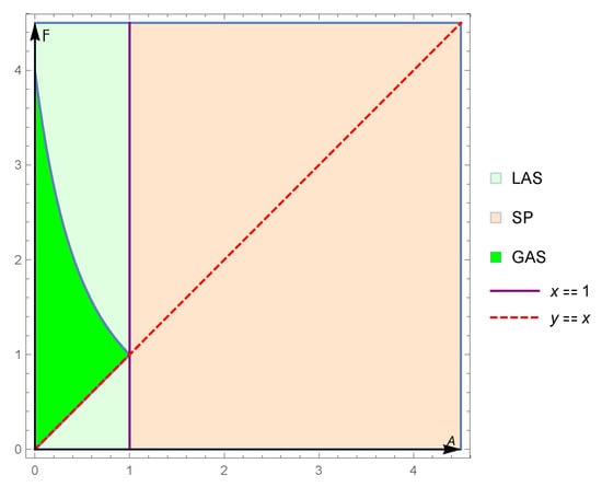
If $0<A<1$ and $A<F\le \frac{4}{{\left(A+1\right)}^2}$, the equilibrium point $\overline{x}$ is globally asymptotically stable (see Figure 2).

Figure 2. The area of the global asymptotic stability (GAS).

Proof. 

Consider the system

$$\begin{array}{c}f\left(m,m\right)=M\\ f\left(M,M\right)=m\end{array}$$

(21)

that is,

$$\begin{array}{c}M{m}^2\left(A+1\right)=m^2+F\\ m{M}^2\left(A+1\right)=M^2+F\end{array}$$

(22)

If we subtract equations of the system (22), we get:

$$\left(m-M\right)mM\left(A+1\right)=\left(m-M\right)\left(m+M\right),$$

so one solution of system (22) is $\left(m,M\right)=\left(\overline{x},\overline{x}\right)$. On the other hand

$$mM\left(A+1\right)=m+M.$$

By adding equations of the system (22), we get:

$$\left(A+1\right)Mm\left(m+M\right)=m^2+M^2+2F.$$

Substitution $mM=q$ and $m+M=p$ leads the system

$$\begin{array}{ccc}\hfill mM\left(A+1\right)& =& m+M\hfill \\ \hfill \left(A+1\right)Mm\left(m+M\right)& =& m^2+M^2+2F\hfill \end{array}$$

to the

$$\begin{array}{ccc}\hfill q\left(A+1\right)& =& p\hfill \\ \hfill \left(A+1\right)pq& =& p^2-2q+2F.\hfill \end{array}$$

If we replace $p=q\left(A+1\right)$ in the second equation, we get

$$q=F$$

so it implies $p=F\left(A+1\right)$. Now, m and M are solutions of equation

$$t^2-pt+q=0.$$

(23)

We get

$$\begin{array}{ccc}\hfill t_{\pm }& =& \frac{p\pm \sqrt{p^2-4q}}{2}=\frac{F\left(A+1\right)\pm \sqrt{F^2{\left(A+1\right)}^2-4F}}{2}\hfill \\ & =& \frac{F\left(A+1\right)\pm \sqrt{F\left(F{\left(A+1\right)}^2-4\right)}}{2}.\hfill \end{array}$$

Equation (23) has no real solutions if $F{\left(A+1\right)}^2-4<0$. For $F{\left(A+1\right)}^2-4=0$, i.e., $F=\frac{4}{{\left(A+1\right)}^2}$ the Equation (23) has solution $m=M=\frac{2}{A+1}=\overline{x}$. Therefore, the system (21) has the unique solution $\left(m,M\right)=\left(\overline{x},\overline{x}\right)$ if $0<A<1$ and $A<F\le \frac{4}{{\left(A+1\right)}^2}$ (because $\frac{4}{{\left(A+1\right)}^2}<\frac{1}{A}$). Now, since $\left[1,\sqrt{\frac{F}{A}}\right]$ is an invariant and attracting interval (by Lemmas 3 and 6), Theorems 3 and 5, the conclusion follows.

Using Theorem 4, we can prove the theorem’s statement without using Lemma 6, i.e., the result of attractivity. Now, we will give another proof.

Every solution of Equation (1) satisfies the fourth order difference equation

$$x_{n+1}=f\left(f\left(x_{n-1},x_{n-2}\right),f\left(x_{n-2},x_{n-3}\right)\right)=f_1\left(x_{n-1},x_{n-2},x_{n-3}\right),n=0,1,\dots ,$$

(24)

where $f_1$ is increasing function in all its arguments. Simplifying the right hand side of Equation (24) we obtain

$$x_{n+1}=\frac{x_{n-2}+A{x}_{n-1}}{F+x_{n-1}{x}_{n-2}}{x}_{n-1}\widehat{G},$$

(25)

where

$$\widehat{G}=\frac{F^2+F{x}_{n-2}\left(A^2{x}_{n-1}^2{x}_{n-2}+A{x}_{n-1}\left(x_{n-3}{x}_{n-1}+x_{n-2}^2\right)+x_{n-1}+x_{n-3}+x_{n-1}{x}_{n-2}{x}_{n-3}\right)+x_{n-1}{x}_{n-2}^2{x}_{n-3}}{F\left(A^2{x}_{n-2}^2+A\left(x_{n-1}^2+x_{n-2}{x}_{n-3}\right)+x_{n-1}{x}_{n-2}\right)+x_{n-1}{x}_{n-2}\left(A^2{x}_{n-2}^2+A{x}_{n-3}\left(x_{n-1}+x_{n-2}\right)+x_{n-2}{x}_{n-3}\right)}.$$

The equilibrium solution of Equation (25) satisfies the equation

$$\left(F-A{x}^3+x^2-x^3\right)\left(-F+Fx-x^2+AFx\right)=0.$$

We conclude that the equilibrium solutions of Equation (25) are either equilibrium solutions of Equation (1) or the solutions of the quadratic equation

$$-F+Fx-x^2+AFx=0.$$

(26)

Equation (26) has no real solutions under the condition: $0<A<1$ and $A<F\le \frac{4}{{\left(A+1\right)}^2}$. Since $\left[1,\sqrt{\frac{F}{A}}\right]$ is an invariant interval for f, and so for $f_1$, an application of Theorem 4 completes the proof. □

Theorem 9.

If $F<A<1$, then every solution of Equation (1) converges to the equilibrium point $\overline{x}$ (see Figure 3).

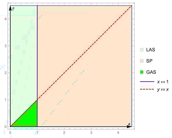
Figure 3. The area of the global asymptotic stability (GAS).

Proof. 

In this region, $f(u,v)$ is decreasing in u and increasing in v. Additionally, by Lemmas 4 and 7, $\left[\sqrt{\frac{F}{A}},1\right]$ is an invariant and attracting interval that contains the equilibrium point $\overline{x}$. By Theorem 1, the subsequences ${\left\{x_{2n}\right\}}_{n=0}^{+\infty }$ and ${\left\{x_{2n+1}\right\}}_{n=0}^{+\infty }$ are eventually monotone. Since they are eventually monotone in $\left[\sqrt{\frac{F}{A}},1\right]$, a bounded interval, they must converge. It is easy to show that in this case, there are no minimal period-two solutions (see Section 3, Lemma 2). Thus every solution of (1) must converge to its unique equilibrium point. □

In case $A>1$, Equation (1) has a unique equilibrium point which is a saddle and unbounded solutions, i.e., dynamic similar as the equation analyzed in [15]. Due to a change of monotonicity, we can only state the following conjecture.

Conjecture 1.

If $A>1$, then every solution of the equation converges to either the equilibrium point $\overline{x}$ or points $\left(0,\infty \right)$, $\left(\infty ,0\right)$. More precisely, every solution which starts of the global stable manifold of the equilibrium $\overline{x}$ converges to the points $\left(0,\infty \right)$, $\left(\infty ,0\right)$.

Conjecture 2.

If $0<A<1$, then the equilibrium point $\overline{x}$ is globally asymptotically stable.

4.2. Case 2 ($A=1$)

Assume that $A=1$ and $F<A$. The function $f\left(u,v\right)$ decreases in the first variable and increases in the second variable on the interval $\left[\sqrt{F},1\right]$.

Lemma 8.

If $F<A=1$, then $\left[\sqrt{F},1\right]$ is an invariant interval of Equation (1), i.e.,

$$f:{\left[\sqrt{F},1\right]}^2\to \left[\sqrt{F},1\right]$$

which contains the equilibrium point $\overline{x}$.

Proof. 

Assume that $F<A=1$. By using that

$$\underset{\left(u,v\right)\in {\left[\sqrt{F},1\right]}^2}{max}f\left(u,v\right)=f\left(\sqrt{F},1\right)=\frac{\sqrt{F}+F}{F+\sqrt{F}}=1,$$

and

$$\underset{\left(u,v\right)\in {\left[\sqrt{F},1\right]}^2}{min}f\left(u,v\right)=f\left(1,\sqrt{F}\right)=\frac{F+\sqrt{F}}{1+\sqrt{F}}=\sqrt{F}$$

the conclusion that $f:{\left[\sqrt{F},1\right]}^2\to \left[\sqrt{F},1\right]$ follows from (20). On the other side, since $F<1$ we obtain

$$\phi \left(\sqrt{F}\right)\phi \left(1\right)=2F\left(\sqrt{F}-1\right)\left(1-F\right)<0.$$

This means that the equilibrium point $\overline{x}$ belongs to the invariant interval $\left[\sqrt{F},1\right]$. □

Theorem 10.

If $0<F<A=1$, then every solution of Equation (1) converges to a minimal period-two solution for $x_{-1},x_0\in \left[\sqrt{F},1\right]$.

Proof. 

By Lemma 8, the function $f\left(u,v\right)$ decreases in the first variable and increases in the second variable on the invariant interval $\left[\sqrt{F},1\right]$. Additionally, by Theorem 5, Theorem 6, and Lemma 2, Equation (1) has unique non-hyperbolic equilibrium point $\overline{x}$ which is unstable and an infinitely many minimal period-two solutions with eigenvalues at the period two point ${\lambda }_1=1$ and ${\lambda }_2\in \left(-1,1\right)$. Notice that $\left(\sqrt{F},1\right)$ and $\left(1,\sqrt{F}\right)$ are minimal period-two solutions, too. Since conditions of Theorem 2 are satisfied on a closed interval, every solution must converge to a minimal period-two solution. □

Conjecture 3.

Let $A=1$. Then for the positive value of F, every solution converges to a minimal period-two solution (see Figure 1).

4.3. Case $A=F<1$

If $A=F$, we have

$$f\left(u,v\right)=\frac{uv+A}{A{u}^2+uv}$$

so the equilibrium point is $\left(\overline{x},\overline{x}\right)=\left(1,1\right)$.

Lemma 9.

Assume that $F=A$. Then the following statements are true:

(a) 

if $x_n\le \overline{x}=1$, then $x_{n+1}\ge \overline{x}=1$,

(b) 

if $x_n>\overline{x}=1$, then $x_{n+1}<\overline{x}=1$.

Proof. 

(a) If $x_n\le 1$, then holds

$$x_{n+1}-1=\frac{x_n{x}_{n-1}+A}{A{x}_n^2+x_n{x}_{n-1}}-1=\frac{x_n{x}_{n-1}+A-A{x}_n^2-x_n{x}_{n-1}}{A{x}_n^2+x_n{x}_{n-1}}=\frac{A\left(1-x_n^2\right)}{A{x}_n^2+x_n{x}_{n-1}}\ge 0,$$

i.e., $x_{n+1}\ge 1$.

(b) The proof is analogous to the previous case. □

In view of Lemma 9 if $x_n<1$ then $x_{n+1}>1$, $x_{n+2}<1$, $x_{n+3}>1,\dots$ for $n=0,1,\dots$. By straightforward calculation, we obtain

$$x_{n+3}-x_{n+1}=\left(x_n-1\right)\frac{F\left(x_n+1\right)\left(F+x_n{x}_{n-1}\right)P_3\left(x_n,x_{n-1},F\right)}{x_n\left(F+x_n{x}_{n-1}+F^2{x}_n+F{x}_{n-1}\right)\left(F{x}_n+x_{n-1}\right)Q_6\left(x_n,x_{n-1},F\right)},$$

where

$$\begin{array}{ccc}\hfill P_3\left(x_n,x_{n-1},F\right)& =& x_{n-1}^3{x}_n^2\left(F+x_n\right){\alpha }_1\left(F,x_n\right)+x_{n-1}^{2}F{x}_n\left(F+x_n\right){\alpha }_2\left(F,x_n\right)\hfill \\ & & +x_{n-1}{F}^2{\alpha }_3\left(F,x_n\right)+F^3{\alpha }_4\left(F,x_n\right),\hfill \end{array}$$

$${\alpha }_1\left(F,x_n\right)=\left(F+1\right)x_n+F\left(1-3F\right),$$

$${\alpha }_2\left(F,x_n\right)=x_n^3\left(2F+1\right)+x_n^{2}F\left(1-6F\right)+x_n\left(F+2\right)+F\left(2-3F\right),$$

$$\begin{array}{ccc}\hfill {\alpha }_3\left(F,x_n\right)& =& F{x}_n^6+x_n^{5}F\left(1-2F\right)+x_n^4\left(2-4F^3+2F\right)+2F{x}_n^3\left(1-2F\right)\hfill \\ & & +x_n^2\left(1-4F^3+2F^2\right)+F\left(3x_n+F-F^2\right),\hfill \end{array}$$

$${\alpha }_4\left(F,x_n\right)=x_n^{5}F\left(1-F^2\right)+x_n^{4}F\left(1-2F\right)+x_n^3\left(1-F^3\right)+x_n{F}^2\left(1-F\right)+F,$$

and

$$\begin{array}{ccc}\hfill Q_6\left(x_n,x_{n-1},F\right)& =& F^3\left(x_{n-1}+F^2\right)x_n^6+F\left(x_{n-1}^2+F\left(2x_{n-1}+3F^2\right)x_{n-1}+F^3\right)x_n^5\hfill \\ & & +x_{n-1}\left(x_{n-1}^2+x_{n-1}F\left(x_{n-1}+3F^2\right)+2F^2\left(F+1\right)\right)x_n^4\hfill \\ & & +\left(F\left(F+1\right)x_{n-1}^3+F\left(F+2\right)x_{n-1}^2+F^3\right)x_n^3\hfill \\ & & +x_{n-1}{F}^2\left(3x_{n-1}+1\right)x_n^2+F^3\left(F+3x_n{x}_{n-1}\right).\hfill \end{array}$$

Using the inequality $x_n>0$, we get

$$\begin{array}{ccc}\hfill {\alpha }_1\left(F,x_n\right)& =& \left(F+1\right)x_n+F\left(1-3F\right)>F\left(1-3F\right)>0\mathrm{if}F<\frac{1}{3},\hfill \\ \hfill {\alpha }_2\left(F,x_n\right)& =& x_n\left(x_n^2\left(2F+1\right)+x_{n}F\left(1-6F\right)+\left(F+2\right)\right)+F\left(2-3F\right)>0\mathrm{if}F<\frac{2}{3},\hfill \end{array}$$

since $x_n^2\left(2F+1\right)+x_n\left(F-6F^2\right)+F+2>0$ because its discriminant is always negative for $F<1$. It is obvious ${\alpha }_3\left(F,x_n\right)$ and ${\alpha }_4\left(F,x_n\right)>0$ if $F<\frac{1}{2}$. So, we have $P_3\left(x_n,x_{n-1},F\right)>0$ for $F<\frac{1}{3}$. If $F=\frac{1}{3}$ then

$$\begin{array}{ccc}\hfill P_3\left(x_n,x_{n-1},\frac{1}{3}\right)& =& \frac{4}{9}{x}_{n-1}^3{x}_n^3\left(3x_n+1\right)+\frac{1}{27}{x}_{n-1}^2{x}_n\left(15x_n^4+2x_n^3+20x_n^2+10x_n+1\right)\hfill \\ & & +\frac{1}{243}{x}_{n-1}\left(9x_n^6+3x_n^5+68x_n^4+6x_n^3+29x_n^2+27x_n+2\right)\hfill \\ & & +\frac{1}{729}\left(8x_n^5+3x_n^4+26x_n^3+2x_n+9\right),\hfill \end{array}$$

so $P_3\left(x_n,x_{n-1},F\right)>0$ for $F\le \frac{1}{3}$. Additionally, $Q_6\left(x_n,x_{n-1},F\right)>0$ always.

Notice, if we assume

(a) 

$x_n>1$ then by Lemma 9$x_{n+1}<1$, $x_{n+2}>1$, $x_{n+3}<1,\dots$ for $n=0,1,\dots$, so $x_{n+3}-x_{n+1}>0$ for $F\le \frac{1}{3}$. Namely, if $x_0>1$ the subsequence ${\left\{x_{2k+1}\right\}}_{k=0}^{\infty }$ is increasing and bounded above by $\overline{x}=1$ and the subsequence ${\left\{x_{2k}\right\}}_{k=0}^{\infty }$ is decreasing and bounded below by $\overline{x}=1$.

(b) 

$x_n<1$ then by Lemma 9$x_{n+1}>1$, $x_{n+2}<1$, $x_{n+3}>1,\dots$ for $n=0,1,\dots$, so $x_{n+3}-x_{n+1}<0$ for $F\le \frac{1}{3}$. Namely, if $x_0<1$ the subsequence ${\left\{x_{2k+1}\right\}}_{k=0}^{\infty }$ is decreasing and bounded below by $\overline{x}=1$ and the subsequence ${\left\{x_{2k}\right\}}_{k=0}^{\infty }$ is increasing and bounded above by $\overline{x}=1$.

(c) 

$x_n=1$ then by Lemma 9$x_{n+k}=1$ for $k\ge 1$, $n=0,1,\dots$.

With previous analysis, we have proved the following lemma:

Lemma 10.

Assume that $A=F\le \frac{1}{3}$. Then even indexed and odd indexed subsequences of every solution of the equation are monotonic.

Now we can state the following theorem:

Theorem 11.

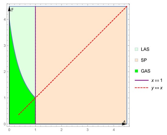
If $A=F\le \frac{1}{3}$, then unique equilibrium point $\overline{x}$ is globally asymptotically stable (see Figure 4).

Figure 4. The area of the global asymptotic stability proved by Theorems 8, 9 and 11.

Proof. 

The proof follows immediately from Lemmas 9 and 10.

□

Remark 1.

If $F>\frac{1}{3}$, then even indexed and odd indexed subsequences of every solution of the equation are eventually monotonic, but at this moment, we can not prove that.

So by Theorem 11 and the number of simulations, we can only state the following conjecture:

Conjecture 4.

If $A=F<1$, then unique equilibrium point $\overline{x}$ is globally asymptotically stable (see Figure 5).

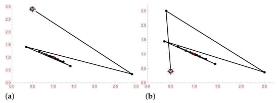
Figure 5. Visualization of Conjecture 4 with $A=F=0.5$ and initial conditions: (a) $\left(x_0,x_{-1}\right)=\left(0.5,2.9\right)$, (b) $\left(x_0,x_{-1}\right)=\left(0.5,0.4\right)$.

References

- Baleanu, D.; Sajjadi, S.S.; Jajarmi, A.; Defterli, Ö. On a nonlinear dynamical system with both chaotic and non-chaotic behaviours: A new fractional analysis and control. Adv. Differ. Equ. 2021, 234, 1–7. [Google Scholar]
- Baleanu, D.; Sajjadi, S.S.; Asad, J.H.; Jajarmi, A.; Estiri, E. Hyperchaotic behaviours, optimal control, and synchronization of a nonautonomous cardiac conduction system. Adv. Differ. Equ. 2021, 157, 1–24. [Google Scholar]
- Khalid, M.; Samikhan, F. Stability analysis of deterministic mathematical model for Zika virus. Br. J. Math. Comput. Sci. 2016, 19, 1–10. [Google Scholar] [CrossRef]
- Rezapour, S.; Mohammadi, H.; Jajarmi, A. A new mathematical model for Zika virus transmission. Adv. Differ. Equ. 2020, 589. [Google Scholar] [CrossRef]
- Kostrov, Y.; Kudlak, Z. On a second-order rational difference equation with a quadratic term. Int. J. Differ. Equ. 2016, 11, 179–202. [Google Scholar]
- Hrustić, S.; Kulenović, M.R.S.; Moranjkić, S.; Nurkanović, Z. Global dynamics of perturbation of certain rational difference equation. Turk. J. Math. 2019, 43, 894–915. [Google Scholar] [CrossRef]
- Nurkanović, Z.; Nurkanović, M.; Garić-Demirović, M. Stability and Neimark-Sacker Bifurcation of Certain Mixed Monotone Rational Second-Order Difference Equation. Qual. Theory Dyn. Syst. 2021, 20, 1–41. [Google Scholar] [CrossRef]
- Bektašević, J.; Kulenović, M.R.S.; Pilav, P. Asymptotic approximations of a stable and unstable manifolds of a two-dimensional quadratic map. J. Comp. Anal. Appl. 2016, 21, 35–51. [Google Scholar]
- Kulenović, M.R.S.; Merino, O. A global attractivity result for maps with invariant boxes. Discret. Contin. Dyn. Syst.-B 2006, 6, 97–110. [Google Scholar] [CrossRef]
- Camouzis, E.; Ladas, G. When does local asymptotic stability imply global attractivity in rational equations. J. Differ. Equ. Appl. 2006, 14, 863–885. [Google Scholar] [CrossRef]
- Kulenović, M.R.S.; Merino, O. Discrete Dynamical Systems and Difference Equations with Mathematica; Chapman and Hall/CRC: Boca Raton, FL, USA; London, UK, 2002. [Google Scholar]
- Kulenović, M.R.S.; Ladas, G. Dynamics of Second Order Rational Difference Equations with Open Problems and Conjectures; Chapman and Hall/CRC: Boca Raton, FL, USA; London, UK, 2001. [Google Scholar]
- Grove, E.A.; Ladas, G. Periodicities in nonlinear difference equations. In Advances in Discrete Mathematics and Applications; Chapman and Hall/CRC: Boca Raton, FL, USA; London, UK, 2005. [Google Scholar]
- Elaydi, S. Discrete Chaos; Chapman and Hall/CRC: Boca Raton, FL, USA; London, UK; New York, NY, USA, 2000. [Google Scholar]
- Garić-Demirović, M.; Hrustić, S.; Moranjkić, S. Global dynamics of certain non-symmetric second-order difference equation with quadratic terms. Sarajevo J. Math. 2019, 15, 155–167. [Google Scholar]
Publisher’s Note: MDPI stays neutral with regard to jurisdictional claims in published maps and institutional affiliations. |
© 2021 by the authors. Licensee MDPI, Basel, Switzerland. This article is an open access article distributed under the terms and conditions of the Creative Commons Attribution (CC BY) license (https://creativecommons.org/licenses/by/4.0/).