Article

Model Predictive Control of COVID-19 Pandemic with Social Isolation and Vaccination Policies in Thailand

by
Jatuphorn Jankhonkhan
1,2 and
Wannika Sawangtong
1,2,*
1
Department of Mathematics, Faculty of Science, Mahidol University, Bangkok 10400, Thailand
2
Centre of Excellence in Mathematics, Commission on Higher Education, Ministry of Education, Bangkok 10400, Thailand
*
Author to whom correspondence should be addressed.
Axioms 2021, 10(4), 274; https://doi.org/10.3390/axioms10040274
Submission received: 22 September 2021 / Revised: 12 October 2021 / Accepted: 15 October 2021 / Published: 25 October 2021
(This article belongs to the Special Issue Mathematics of the COVID-19)

Abstract

:
This study concerns the COVID-19 pandemic in Thailand related to social isolation and vaccination policies. The behavior of disease spread is described by an epidemic model via a system of ordinary differential equations. The invariant region and equilibrium point of the model, as well as the basic reproduction number, are also examined. Moreover, the model is fitted to real data for the second wave and the third wave of the pandemic in Thailand by a sum square error method in order to forecast the future spread of infectious diseases at each time. Furthermore, the model predictive control technique with quadratic programming is used to investigate the schedule of preventive measures over a time horizon. As a result, firstly, the plan results are proposed to solve the limitation of ICU capacity and increase the survival rate of patients. Secondly, the plan to control the outbreak without vaccination shows a strict policy that is difficult to do practically. Finally, the vaccination plan significantly prevents disease transmission, since the populations who get the vaccination have immunity against the virus. Moreover, the outbreak is controlled in 28 weeks. The results of a measurement strategy for preventing the disease are examined and compared with a control and without a control. Thus, the schedule over a time horizon can be suitably used for controlling.

1. Introduction

COVID-19 is a new disease that appeared at the end of 2019 and is caused by the virus severe acute respiratory syndrome coronavirus 2 (SARS-CoV-2). The virus spreads to others if they come into contact with respiratory droplets or aerosols of infected people through coughing, sneezing, or talking, as well as through close contact or sharing items with an infected person [1,2]. Infected individuals can present symptoms or be asymptomatic [3]. Some studies have suggested the proportion of infected people who show symptoms is eighty percent, with asymptomatic individuals accounting for twenty percent [4]. Fever, dry cough, and fatigue are among the most common symptoms of people who are infected and show symptoms [5]. After people get the virus, they can detect the infection and show symptoms after 2–14 days, which is the incubation period of COVID-19 [6].
The COVID-19 pandemic began in December 2019 in Wuhan, China. It continued to spread around the world and has killed millions of people, as shown in the report of the World Health Organization (WHO) [7]. The total number of infected people and deaths worldwide was 210,805,121 and 4,416,421, respectively. The data were last updated on 19 August 2021. Aside from the epidemic having a negative impact on the health of people, it has affected education, the economy, human life, and others. For example, laying off employees because of lockdown measures that forced businesses to close, testing the effectiveness of online education during the pandemic, and food security. Therefore, locking down, social distancing, wearing a face mask, and working from home were preventive measures to be used to prevent the transmission of the COVID-19 pandemic in many countries. For example, a survey of more than 2000 adults in the United States reported that 72 percent intend to continue wearing face masks in public, 88 percent intend to avoid crowds, and 50 percent intend to frequently wash their hands and use hand sanitizer [8]. A vaccine to prevent COVID-19 infection was developed, and the mRNA vaccine, the Pfizer/BioNTech vaccine, was the first to receive emergency validation from the World Health Organization (WHO). Now, the WHO has evaluated the following vaccines: AstraZeneca/Oxford, Johnson and Johnson, Moderna, Pfizer/BioNTech, Sinopharm, and Sinovac, against COVID-19 infection. These vaccines were used in many countries to reduce the number of infected people [9,10].
The COVID-19 epidemic has already spread to Thailand in three waves. The first wave of the outbreak began in January 2020, with a peak of 188 infected patients per day, and was finally brought under control in March, while the second wave started in November 2020, with a rise in infected populations that reached 800 cases a day, before decreasing in March 2021. Furthermore, the third wave started in April 2021. On 19 August 2021, the number of newly infected cases and death cases each day was higher than in the preceding two waves, with 20,902 cases and 235 cases, respectively. The data were reported by Thailand’s Ministry of Public Health’s Department of Disease Control and the World Health Organization (WHO) [11,12]. The total number of infected cases in Thailand was 989,859, with 8586 deaths. Social isolation policies, such as social distancing and the use of face masks, were used to control the epidemic in the three waves. Furthermore, a vaccine against COVID-19 infection became critical for the control of disease spread in the third wave, which was mostly limited to healthcare workers and relied primarily on the Sinovac Biotech vaccine. The vaccine was imported from China. The advantage of this vaccine is the reduction in the risk of death from infection. In contrast, the efficiency of preventing the virus is lowest compared with other kinds of vaccine, such as the Oxford–AstraZeneca vaccine. The Oxford–AstraZeneca vaccine was planned to be administered to the majority of the population to prevent COVID-19 infections [13]. Thus, this vaccine is investigated in this work.
In order for people to live a normal life, the outbreak should be resolved. Furthermore, efficient management can mitigate damage during a pandemic. Therefore, the application of mathematical fields is used to study the pandemic and compute a suitable plan for preventive measures.
Mathematical modeling is one of the applications that can be used for solving real-world problems. It can be applied to study and predict the behavior of outbreaks via a system of nonlinear differential equations, such as the models of influenza, Ebola, and coronavirus diseases by [4,14,15]. Now, epidemic models have been developed. Chancharoenthana Wiwat et al. used the S I R model (Susceptible–Infected–Recovered) to study the COVID-19 pandemic and examined the contacts and the recovery of exposed and infected individuals [16]. After that, the S I R model was extended and then became the S E I R model (Susceptible–Exposed–Infected–Recovered). Natcha C Jitsuk et al. examined the impact of Thailand’s Songkran festival on COVID-19 transmission by using this model [17]. Thus, the incubation period of the disease was considered in the model. Moreover, the kinds of populations were determined and then the model was improved. The contact between and recovery of exposed and infected populations, symptomatic and asymptomatic infected populations, were focused on by T D Frank et al. and Robert C. Reiner Jr et al. [18,19]. In addition, Saulo B. Bastos et al. studied the number of death cases and predicted the early evolution of the COVID-19 pandemic in Brazil [20]. Furthermore, a quarantine was applied in an epidemic model to establish its association between infection and the control of disease spread. Enahoro Iboi et al. organized the classical model to assess the effectiveness of public health education campaigns during the COVID-19 pandemic in the United States. This model concerns the isolation and non-isolation of people, as well as the number of hospitalized and non-hospitalized individuals [21], and Pakwan Riyapan et al. concentrated on the isolation of infected people. Calistus N. Ngonghala et al. focused on the isolation of non-infected and infected people, and looked into using the quarantine model to resolve the COVID-19 pandemic. They used sensitivity analysis to investigate the interaction of the outbreak and the parameters of transmission, quarantine, and contact tracing [4,22].
The S E I R model was depicted by fractional models in order to investigate disease transmission. For example, Saheed O. Akindeinde et al. used the fractional model to study the interaction of humans and pathogens, Olaniyi Iyiola et al. used the model to focus on the quarante of exposed and infected populations [23,24], and Isaac Owusu-Mensah et al. organized the model to investigate the rates of transmission, testing, and the transition of asymptomatic to symptomatic infected people and then continued to examine the impact of the rates on the outbreak [25]. Moreover, social isolation measures were studied in the model of the COVID-19 pandemic in Wuhan, Italy, and the United States, as well as the first and second waves of the outbreak in Thailand [4,26,27,28,29].
The optimum control theory is a method used to solve dynamic problems. It is a method used for the minimization of the cost function while computing control variables, for instance, applying optimal control of continuous-time and discrete-time in epidemic models. Pontryagin’s maximum was used to study the swine influenza disease, and model predictive control (MPC) was used to solve the Atopic Dermatitis (AD) model [14,30]. Moreover, quadratic programming is also being studied for use in the solving of constraint problems [31,32].
In this work, the mathematical model was developed from the model by Calistus N.Ngonghala et al. in order to study the second and third waves of the pandemic in Thailand [4]. The model focused on social distancing and vaccination policies, as well as the parameters of transmission, quarantine, and contact tracing. Model predictive control was used to solve discrete-time models. The technique provided the results of controlled variables over a time horizon. The results are suitable for a large group of people to use in reality when compared with the results of the continuous-time model. The idea of the technique was to compute control variables that can control the output of the system to reach a set point.
The research constructed a mathematical model to examine the COVID-19 pandemic concerning prevention strategies. The model, as well as the model’s analysis, invariant regions, equilibrium point, and the basic reproduction number, are all presented in Section 2. Section 3 investigates model predictive control, including linearization and discretization algorithms. In addition, Section 4 exhibits the curve fitting of the COVID-19 pandemic in Thailand and the pandemic’s prevention strategies. In the discussion and conclusion sections, the work is summarized.

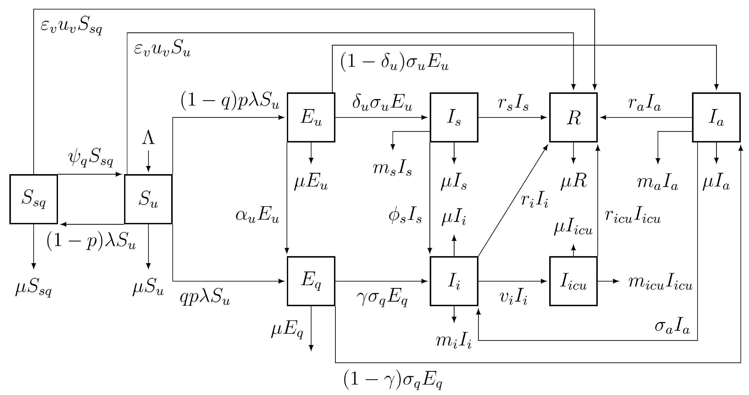
2. Mathematical Model

The mathematical model of the COVID-19 pandemic is described in this section, followed by an analysis of the model that includes the invariant region, equilibrium points, and the basic reproduction number.
The disease transmission of the COVID-19 pandemic is illustrated by the flow diagram in Figure 1. The nine components in the diagram represent the kinds of populations. Non-quarantined susceptible ( S u ), quarantined susceptible ( S s q ), who are quarantined in state quarantine, non-quarantined exposed ( E u ), quarantined exposed ( E q ), exposed individuals who are infected but do not show symptoms and can not transmit infection, symptomatically-infectious ( I s ), who are infected and show the symptoms of COVID-19, asymptomatically-infectious ( I a ), who infected but exhibiting mild or no clinical symptoms of COVID-19, isolated infectious ( I i ), who isolated in hospitals and state quarantine and isolated infections require intensive care unit ( I i c u ), as well as recovered individuals (R) at any time t. Moreover, the total population (N) is defined by
N ( t ) = S u ( t ) + S s q ( t ) + E u ( t ) + E q ( t ) + I s ( t ) + I i ( t ) + I a ( t ) + I i c u ( t ) + R ( t ) .
Moreover, the model is given as the system of a nonlinear differential equation in the following:
S ˙ u = Λ ( ( 1 p ) + ( 1 q ) p + q p ) λ S u ( t ) + ψ q S s q ( t ) μ S u ( t ) ε v u v S u ( t ) ,
S ˙ s q = ( 1 p ) λ S u ( t ) ( ψ q + μ ) S s q ( t ) ε v u v S s q ( t ) ,
E ˙ u = ( 1 q ) p λ S u ( t ) ( σ u + α u + μ ) E u ( t ) ,
E ˙ q = q p λ S u ( t ) + α u E u ( t ) ( σ q + μ ) E q ( t ) ,
I ˙ s = δ u σ u E u ( t ) ( r s + ϕ s + m s + μ ) I s ( t ) ,
I ˙ i = γ σ q E q ( t ) + ϕ s I s ( t ) + σ a I a ( t ) ( r i + v i + m i + μ ) I i ( t ) ,
I ˙ a = ( 1 δ u ) σ u E u ( t ) + ( 1 γ ) σ q E q ( t ) ( r a + σ a + m a + μ ) I a ( t ) ,
I ˙ i c u = v i I i ( t ) ( r i c u + m i c u + μ ) I i c u ( t ) ,
R ˙ = r s I s ( t ) + r i I i ( t ) + r a I a ( t ) + r i c u I i c u ( t ) μ R ( t ) + ε v u v S u ( t ) + ε v u v S s q ( t ) ,
where force of infection, λ , and initial condition, I C , are defined by
λ = β s o ( 1 u s o ) ( 1 u M ) ( I s ( t ) + η a I a ( t ) ) S u ( t ) + E u ( t ) + I s ( t ) + I a ( t ) + R ( t ) ,
and
I C = [ S u ( 0 ) S s q ( 0 ) E u ( 0 ) E q ( 0 ) I s ( 0 ) I i ( 0 ) I a ( 0 ) I i c u ( 0 ) R ( 0 ) ] T .
In addition, the number of deaths in the population (D) is
D ˙ = m s I s ( t ) + m i I i ( t ) + m a I a ( t ) + m i c u I i c u ( t ) .
The parameters u s o , u M and u v represent the effect of social distancing, the use of face masks and vaccination, ( 0 u s o , u M , u v 1 ) , which are set as constant, while u v is set as zero. The parameter Λ is the recruitment rate, μ is the natural mortality rate and p λ is the rate of getting the virus with the probability of infection, p. In the susceptible classes, the non-quarantined populations are quarantined at a rate ( 1 p ) λ , and they are released from quarantine and reversed to the non-quarantine class at a rate ψ q . Moreover, they move to the exposed classes with and without quarantine at the rates q p λ and ( 1 q ) p λ , respectively, with the rate of quarantined, q. In the exposed class, there is no disease transmission because it is during the incubation stage of the virus. The incubation periods of non-quarantine and quarantine are defined by σ u and σ q , respectively. The non-quarantined populations are quarantined at the rate of α u , contact tracking rate, and they move to the symptomatic and asymptomatic infectious classes at the rates δ u σ u and ( 1 δ u ) σ u , respectively, at the end of the incubation period. In addition, the quarantined populations also move to the symptomatic and asymptomatic infectious classes at the rates γ σ q and ( 1 γ ) σ q , respectively, at the end of the incubation period. In infected classes, the symptomatic and asymptomatic infectious populations are isolated by contact tracking at the rate ϕ s and σ a , respectively. Furthermore, the isolated people move to the intensive care unit classes at the rate v i . Next, the recovery rates and mortality rates due to the COVID-19 pandemic of the infected classes, I s , I i , I a , and I i c u , are defined by r s , r i , r a , r i c u and m s , m i , m a , m i c u . Moreover, the susceptible population will have immunity against the disease at the rate ε v u v with vaccine efficacy, ε v .

2.1. Invariant Region

Invariant region is the method used for the study of the non-negative of all components of the model (1); it is shown in the following Theorem.
Theorem 1.
Suppose that the initial value I C in Equation (3) is all non-negative. Then, the solution of model (1) that start with these initial values will remain non-negative for all time t > 0 . Furthermore, all solutions of the model (1) are bounded.
Proof of Theorem 1.
Suppose δ min { m s , m i , m a , m i c u } and d min { μ , δ } .
N ˙ = Λ μ N m s I s m i I i m a I a m i c u I i c u Λ μ ( S u + S s q + E u + E q + R ) ( μ + δ ) ( I s + I i + I a + I i c u ) Λ d ( S u + S s q + E u + E q + R ) d ( I s + I i + I a + I i c u ) Λ d N ,
then lim sup t N ( t ) Λ d , namely all solutions are non-negative. □
Theorem 2.
The region Γ = { ( S u ( t ) , S s q ( t ) , E u ( t ) , E q ( t ) , I s ( t ) , I i ( t ) , I a ( t ) , I i c u ( t ) , R ( t ) ) R + 9 : N ( t ) Λ d } is positively invariant for the model (1) for every non-negative initial condition in R + 9 .
From the above, the components of the model in Equation (1) satisfy Theorems 1 and 2; then, they are non-negative.

2.2. The Equilibrium Points

The equilibrium points of the model (1) yield two points: a disease-free equilibrium point ( E d f e ) and an endemic equilibrium point ( E e e ), which are given by the following equations:
  • Disease-free equilibrium point E d f e :
    E d f e = S u , S s q , E u , E q , I s , I i , I a , I i c u , R = Λ μ , 0 , 0 , 0 , 0 , 0 , 0 , 0 , 0 .
  • Endemic equilibrium point E e e :
    E e e = S u * , S s q * , E u * , E q * , I s * , I i * , I a * , I i c u * , R * ,
    where
    S u * = Λ + ψ q S s q * A 1 λ * + μ , S s q * = ( 1 p ) λ * S u * A 2 , E u * = ( 1 q ) p λ * S u * A 3 , E q * = q p λ * S u * + α u E u * A 4 , I s * = δ u σ u E u * A 5 , I i * = γ σ q E q * + ϕ s I s * + σ a I a * A 6 , I a * = A 7 E u * + E q * σ q ( 1 γ ) A 8 , I i c u * = v i I i * A 9 , R * = r s I s * + r i I i * + r a I a * + r i c u I i c u * μ , λ * = A 0 ( I s * + η a I a * ) S u * + E u * + I s * + I a * + R * ,
    and A 0 = β s o ( 1 u s o ) ( 1 u M ) , A 1 = ( 1 p ) + ( 1 q ) p + q p , A 2 = ψ q + μ , A 3 = σ u + α u + μ , A 4 = σ q + μ , A 5 = r s + ϕ s + m s + μ , A 6 = r i + v i + m i + μ , A 7 = ( 1 δ u ) σ u , A 8 = r a + σ a + m a + μ , A 9 = r i c u + m i c u + μ .

2.3. The Basic Reproduction Number R 0

The basic reproduction number is used to explain disease spread, the effectiveness of contact rate, the risk of infection, and the length of infectiousness by comparing the average number of newly infected cases with the number of infected cases in a community. The basic reproduction number of a model can be investigated by using the next-generation matrix method.
The method focuses on using the disease-free equilibrium point and the Jacobian matrix to apply a spectral radius theory to the infected components of a model. So, a subsystem of the model (1) concerning the states-at-infection form is the models (1c)–(1h). It can be rewritten as
x ˙ = F ( x ) V ( x ) ,
where
F ( x ) = A 0 S u p I a η a + I s q 1 E u + I a + I s + R + S u A 0 S u p q I a η a + I s E u + I a + I s + R + S u 0 0 0 0 , V ( x ) = A 3 E u A 4 E q E u α u E u δ u σ u + A 5 I s γ E q σ q + A 6 I i I a σ a I s ϕ s A 7 E u + A 8 I a + E q σ q γ 1 A 9 I i c u I i v i ,
and x = [ E u E q I s I i I a I i c u ] T . Next, the spectral radius of the matrix, J F ( E d f e ) J V 1 ( E d f e ) , is defined by
ρ ( J F ( E d f e ) J V 1 ( E d f e ) ) = max i = 1 , 2 , , n e | e i | ,
where e j are eigenvalues of the matrix and n e is number of the eigenvalues [33,34]. The matrix J F ( E d f e ) and J V ( E d f e ) are Jacobian matrices of the matrix F ( x ) and the matrix V ( x ) at the disease-free equilibrium point, E d f e . Thus,
J F ( E d f e ) = 0 0 A 0 p q 1 0 A 0 η a p q 1 0 0 0 A 0 p q 0 A 0 η a p q 0 0 0 0 0 0 0 0 0 0 0 0 0 0 0 0 0 0 0 0 0 0 0 0 0
and
J V ( E d f e ) = A 3 0 0 0 0 0 α u A 4 0 0 0 0 δ u σ u 0 A 5 0 0 0 0 γ σ q ϕ s A 6 σ a 0 A 7 σ q γ 1 0 0 A 8 0 0 0 0 v i 0 A 9 .
Therefore, the basic reproduction number, R 0 , of the model (1) is denoted by:
R 0 = p A 0 A 3 A 4 A 5 A 8 ( ( 1 γ ) A 5 η a σ q ( A 3 q α u q + α u ) + A 4 ( 1 q ) ( A 5 A 7 η a + A 8 δ u σ u ) ) .
Theorem 3.
The endemic equilibrium is locally stable in the feasible region (1) if R 0 > 1 [35].
The theorem above establishes a connection between the basic reproduction number and the model’s convergence.
Next, the methodology for controlling the disease, model predictive control (MPC), is discussed, as well as linearized and discretized methods.

3. Model Predictive Control (MPC)

In this section, we look into model predictive control (MPC), which uses the optimum control theory method to obtain the optimal control variables for minimizing the cost function and predicting future output over a time horizon. In addition, the state-space model is generated in the application, and linearization and discretization methods will be used to provide it.

3.1. Linearization and Discretization

The linearization method associated with a Taylor expansion and the exact discretization technique are discussed. The first method is used to convert the model to a linear model, while the second method is used to convert it from a continuous-time model to a discrete-time model.
First, the mathematical model (1) given in continuous time by a system of nonlinear differential equations can be rewritten as
x ˙ ( t ) = f ( x ( t ) , u ( t ) ) ,
where x is the vector of system state, x ( t ) = [ S u ( t ) S s q ( t ) E u ( t ) E q ( t ) I s ( t ) I i ( t ) I a ( t ) I i c u ( t ) R ( t ) ] T , u ( t ) is the vector of control input, u ( t ) = [ u s o ( t ) u M ( t ) u v ( t ) σ a ( t ) α u ( t ) q ( t ) ] T , x ˙ ( t ) is the vector of the derivative of the system state at time t and f is a function of the state and input variables of the system.
Let ( x s , u s ) be an equilibrium point, i.e., f ( x s , u s ) = 0 , the equilibrium points of the model (1), x s = E e e , the endemic equilibrium point. Furthermore, the initial steady state of the control vector is set as u s = [ 0 0 0 σ a α u q ] T . Applying Taylor expansion around the equilibrium point [36],
x ˙ ( t ) = f ( x ( t ) , u ( t ) ) f ( x s , u s ) + f x ( x s , u s ) ( x ( t ) x s ) + f u ( x s , u s ) ( u ( t ) u s ) = A c δ x ( t ) + B c δ u ( t ) , x ˙ ( t ) = d x ( t ) d t = d ( x ( t ) x s ) d t = d δ x ( t ) d t = δ x ˙ ( t ) .
Therefore, the linear model is
δ x ˙ ( t ) = A c δ x ( t ) + B c δ u ( t ) ,
where A c = f x ( x s , u s ) , B c = f u ( x s , u s ) , δ x ( t ) = x ( t ) x s and δ u ( t ) = u ( t ) u s .
Next, the linear model in Equation (11) is discretized by the exact discretization method, which is defined by
δ x ( k + 1 ) = A d δ x ( k ) + B d δ u ( k ) ,
where T s is the sampling period of time, k is discrete-time, A d = e A c T s and B d = 0 T s e A c τ d τ B c = A c 1 ( e A c T s I ) B c [32]. Finally, the linearized discrete time state-space model of Equation (12) can be rewritten as
x ( k + 1 ) = A d x ( k ) + B d u ( k ) , y ( k ) = C x ( k ) ,
where x is the state vector, u is the input vector and y is the output vector, with C the matrix indicating the measure state.

3.2. Cost Function of the Model Predictive Control, J ( k )

The cost function of model predictive control for constrained problems is defined by
J ( k ) = [ Y ( k ) X s p ] T W y [ Y ( k ) X s p ] + U T ( k ) W u U ( k ) , s . t . x ( k + 1 ) = A d x ( k ) + B d u ( k ) , y ( k ) = C x ( k ) , u min u ( k ) u max ,
where U ( k ) = U ( k ) U ( k 1 ) , Q y = d i a g ( w y i ) , Q u = d i a g ( w u j ) , W y = I N p Q y , W u = I N p Q u and X s p = 1 N P x s p T . The parameters n y and n u are the number of output and control variables, w y i , ( i = 1 , 2 , . . . , n y ) is the weight of output variables and w u i , ( i = 1 , 2 , . . . , n u ) is the weight of control variables. W y is the weight matrix of the vector, which is the error between the output and the set-point, W u is the weight matrix of control vector, x s p is target vector or set-point, u min is the minimum of control vector, u max is the maximum of control vector and ⊗ is Kronecker product [32].
The cost function, J ( k ) , can be transformed into a quadratic programming form, as defined by the equation below:
min U ( k ) J ( k ) = 1 2 U T ( k ) H q p U ( k ) + U T ( k ) G q p , H q p = H y + H u , G q p = G y + G u , s . t . A e q U ( k ) B e q ,
where H y = 2 ϕ T W x ϕ , H u = 2 H Q u , G y = 2 ( ϕ T W x F x ( k 1 ) ϕ T W x X s p ) , G u = M u u ( k 1 ) , U min = 1 N P u min and U max = 1 N P u max . The matrix A e q and the matrix B e q are defined by
A e q = I m O O O I m O O O O I m O O O I m O O O O I m O O O I m O O O O I m O O O I m and B e q = u max u min u max u min u max u min u max u min ,
where I m is an identity matrix dimension m and O is a zero matrix dimension m when m is dimension of control vector u .
Next, the COVID-19 epidemic in Thailand is numerically simulated. In addition, the model is subjected to the application of control theory, namely model predictive control.

4. Results

In this section, the baseline parameter values reported in Table 1 and the initial conditions ( I C ), S u ( 0 ) = 66,189,981, S s q ( 0 ) = 0 , E u ( 0 ) = 15 , E q ( 0 ) = 0 , I s ( 0 ) = 1 , I i ( 0 ) = 0 , I a ( 0 ) = 3 , I i c u ( 0 ) = 0 and R ( 0 ) = 0 , are utilized to fit the model parameters to real data from the COVID-19 pandemic in Thailand. In order to forecast future disease spread behavior, the model parameters are fitted using the sum square error method and the parameters, β s o , p , σ a , α u , and q are computed. Moreover, the model predictive control technique with quadratic programming is used to determine the schedule of COVID-19 disease prevention interventions. The weight matrix of social isolation and vaccination policies are assumed to be 0.01, and the prediction horizon, N p , is 35.

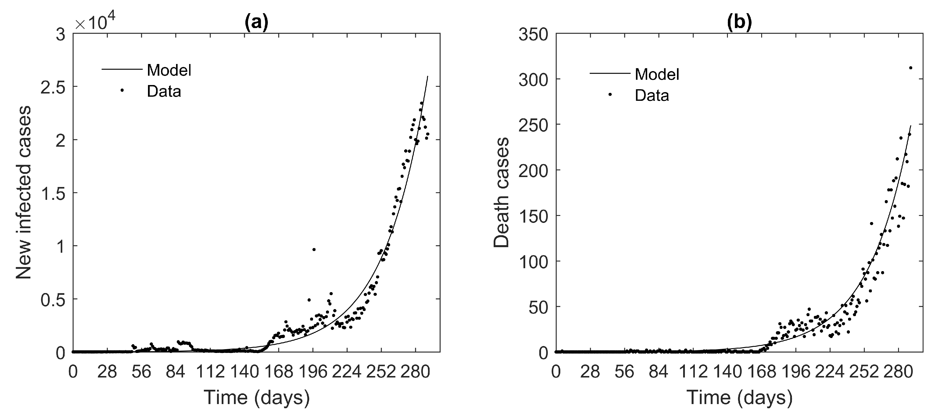
4.1. Mathematical Modeling of COVID-19 Pandemic in Thailand

The COVID-19 pandemic in Thailand is shown in Figure 2. The solid line displays the model’s curve fitting, whereas the dotted line depicts real data during the COVID-19 pandemic in 290 days, from 1 November 2020 to 19 August 2021. The data of newly infected cases in Figure 2a and death cases in Figure 2b are reported by Thailand’s Ministry of Public Health’s Department of Disease Control [11]. In addition, the sum square error method is used to evaluate several parameters in the model (1) relevant to the scenario of disease transmission in Thailand. Thus, parameter values, β s o = 0.9519 , p = 0.8891 , σ a = 0.2533 , α u = 0.0326 and q = 0.0397 , are obtained. Moreover, the basic reproduction number, R 0 , is calculated as 1.23.
The model parameters were obtained. So, the pandemic trajectory was predicted for 28 weeks later. Figure 3 presents the prediction of infected populations with and without measures, contact tracing of asymptomatic infected and non-quarantined exposed people, as well as the quarantine of non-quarantined susceptible people in the black lines and the red lines. The rise in infected populations is depicted in Figure 3a, with the biggest peak in the number of isolated infected populations, which can affect hospital bed shortages. Furthermore, as time passes, the graph will continue to fluctuate and converge to the endemic equilibrium point. Hence, the results satisfy Theorem 3 for R 0 > 1 . In addition, the effectiveness of preventive measures is shown in Figure 3b. The number of infected populations in the graph without control is higher than in the graph with control. Hence, a lot of people will be infected and die because of the pandemic.

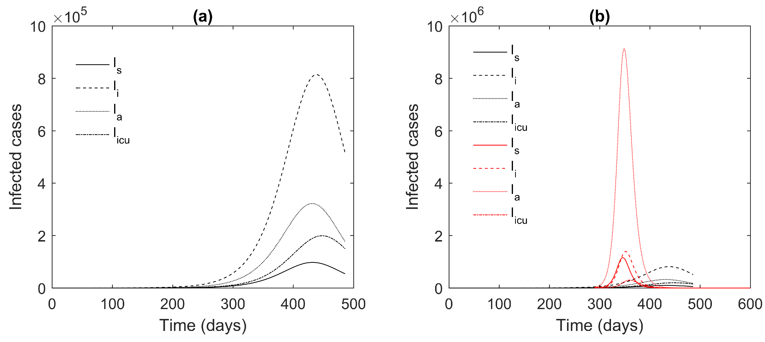
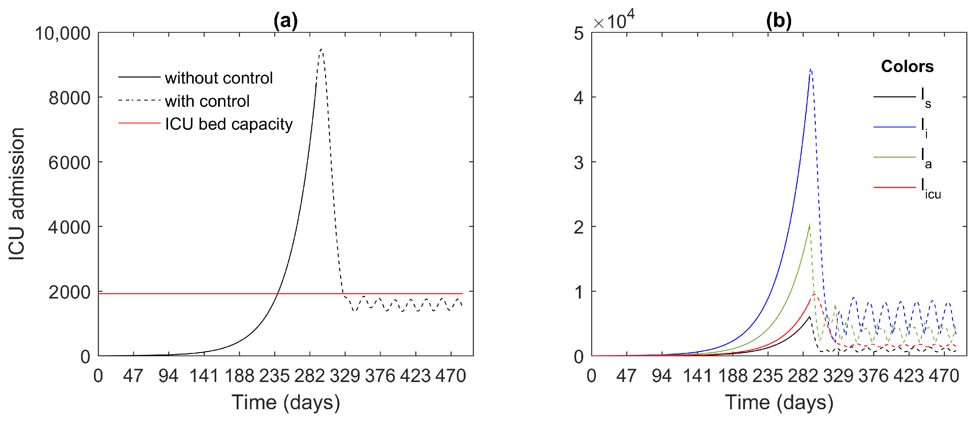
4.2. ICU Capacity Restriction and the Effectiveness of Social Isolation Strategies

The results of some components from Figure 3 may be contradictory with the true situation, particularly the number of patients in critical care units (ICUs). The number of ICU admissions is influenced by ICU bed capacity due to ICU bed limits. This means that some patients will have a significant risk of death if they are not treated in an ICU room. In addition, if there are fewer options for increasing the number of ICU beds, the number of serious patient cases must be reduced. Assume that there are roughly 1920 ICU beds available for COVID-19 patients, and set it as a set-point [41]. The model predictive control is then used to create a plan for social isolation regulations in order to keep the number of intensive care unit patients under control.
The 28 weeks of outbreak prediction of infected populations is examined in Figure 4. The solid line in Figure 4a depicts the curve fitting of ICU cases in Thailand. The dashed line depicts the number of ICU admissions, which is influenced by the red line’s capacity for ICU beds. The number of patients is lowered until it is near to the number of ICU beds available, at which point social isolation measures are used to manage the oscillation and convergence to the set-point. As demonstrated in Figure 4b, this result in Figure 4a has an impact on the number of other infected populations.
Figure 5 shows the strategy for preventive measures without vaccination for each week. So, the vaccination rate is set at zero in Figure 5c. The ranges of social distancing and the use of face masks are set between zero and one, while the ranges of σ a , α u , and q are set in zero and their estimated values are shown in Table 1. Moreover, the plan is shown under the relaxation of contact tracing and quarantine. The results pay attention to social distancing and the use of face masks for controlling disease transmission.
Despite the fact that a reduction in the number of patients in ICU classes and all infected people increases the chances of survival, the risk of mortality and the number of infected people remain high. As a result, the effect of managing the epidemic by reducing the number of affected people is investigated.

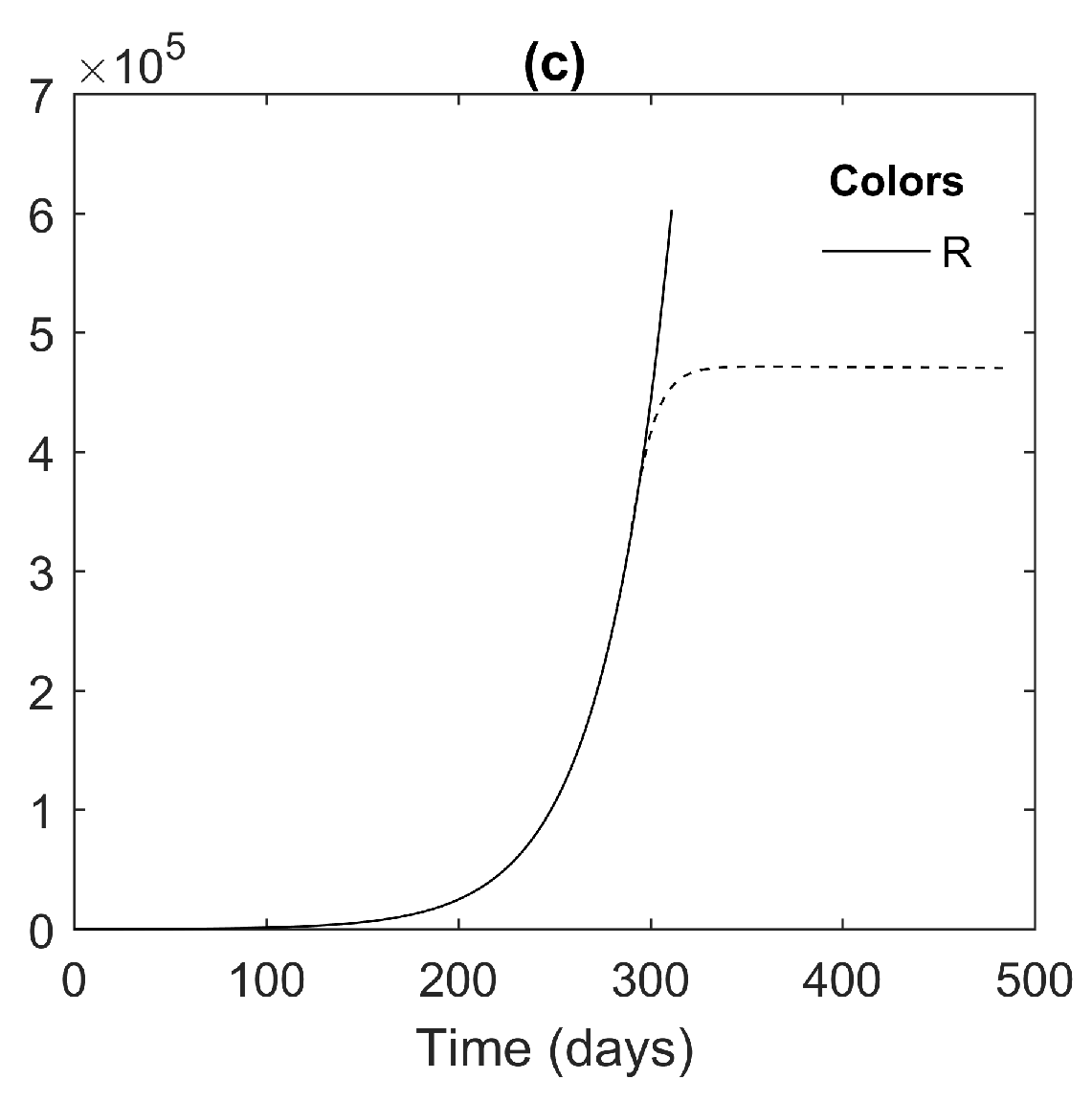
4.3. The Effectiveness of the Social Isolation Policy in Reducing COVID-19 Pandemic Transmission

Figure 6 illustrates the results of the numbers of infected, susceptible, and recovered populations in Figure 6a,b,c, respectively. The solid lines represent the behavior of a growing population when it is out of control. The dashed lines, on the other hand, depict a population reduction due to control measures. In addition, the effectiveness of social isolation strategies in disease control has led to a reduction in the numbers of infected populations, symptomatic infected, isolated infected, and asymptomatic infected populations, as well as of people in the intensive care unit. The trends of all graphs decrease and approach zero. Moreover, the results of susceptible and recovered populations show a decreasing risk of infection among people.
The measuring plans for each of the two weeks of social isolation strategies without vaccination are shown in Figure 7. The proportions of all social isolation policies are bound by one. The figure suggests the plan for the guidelines aimed at strictly controlling the disease. The plan implies that the disease spread of the COVID-19 pandemic will be controlled if people continue to practice social isolation measures for the rest of their lives. Hence, the policies are good to use for a short time but are unsuitable for dealing with the epidemic over a lengthy period of time.

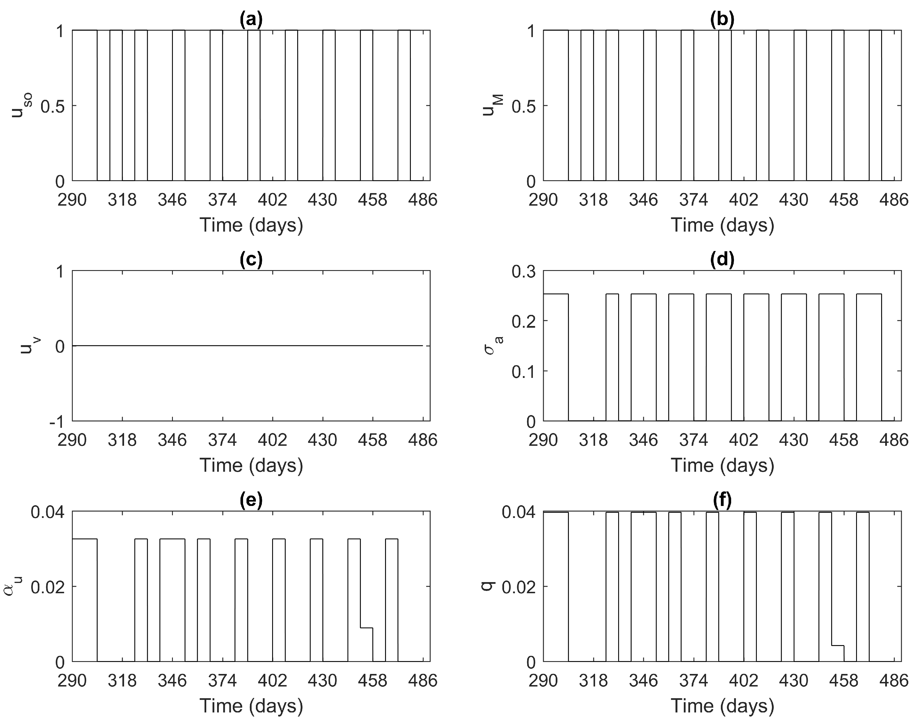
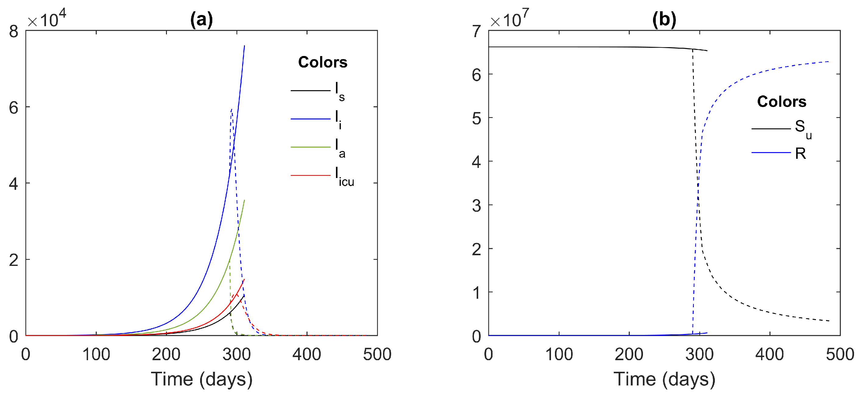
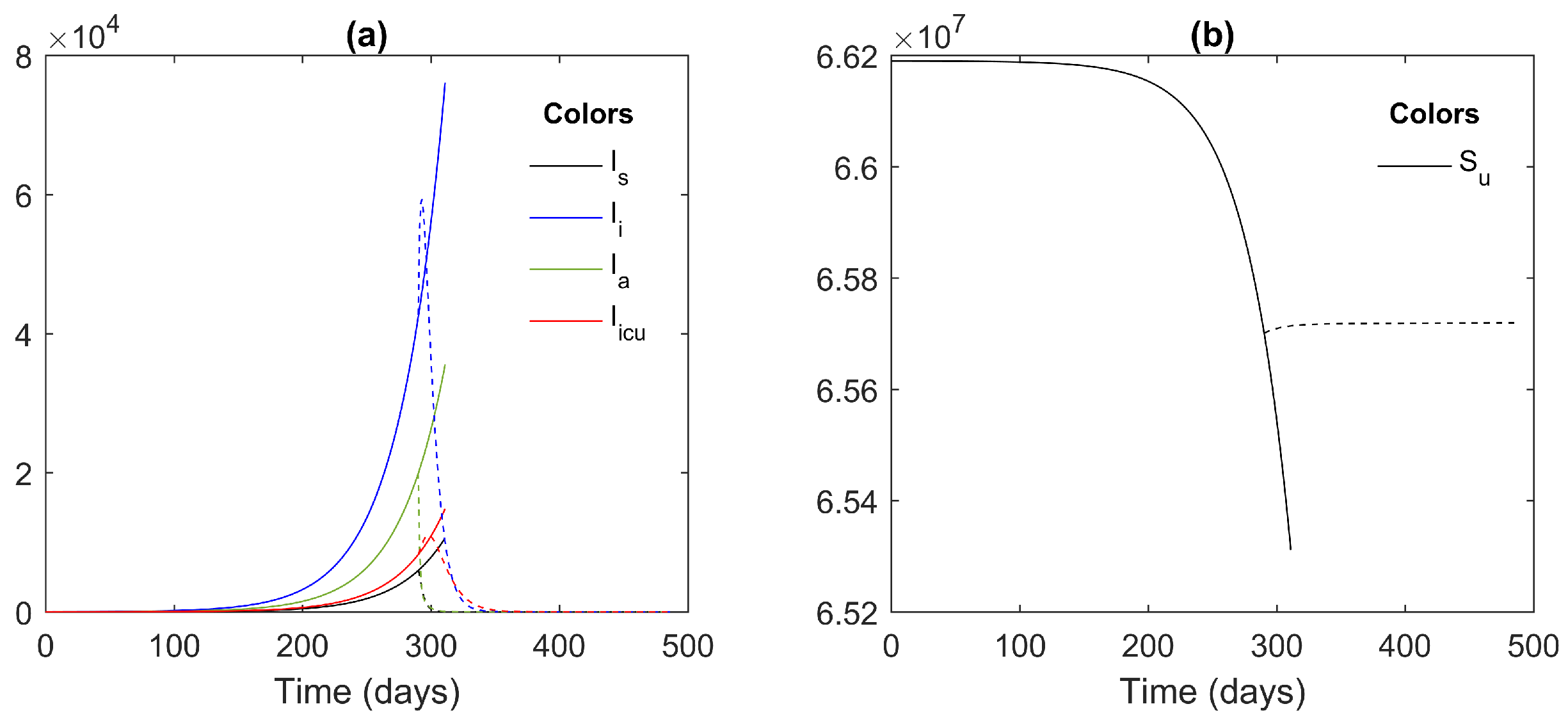
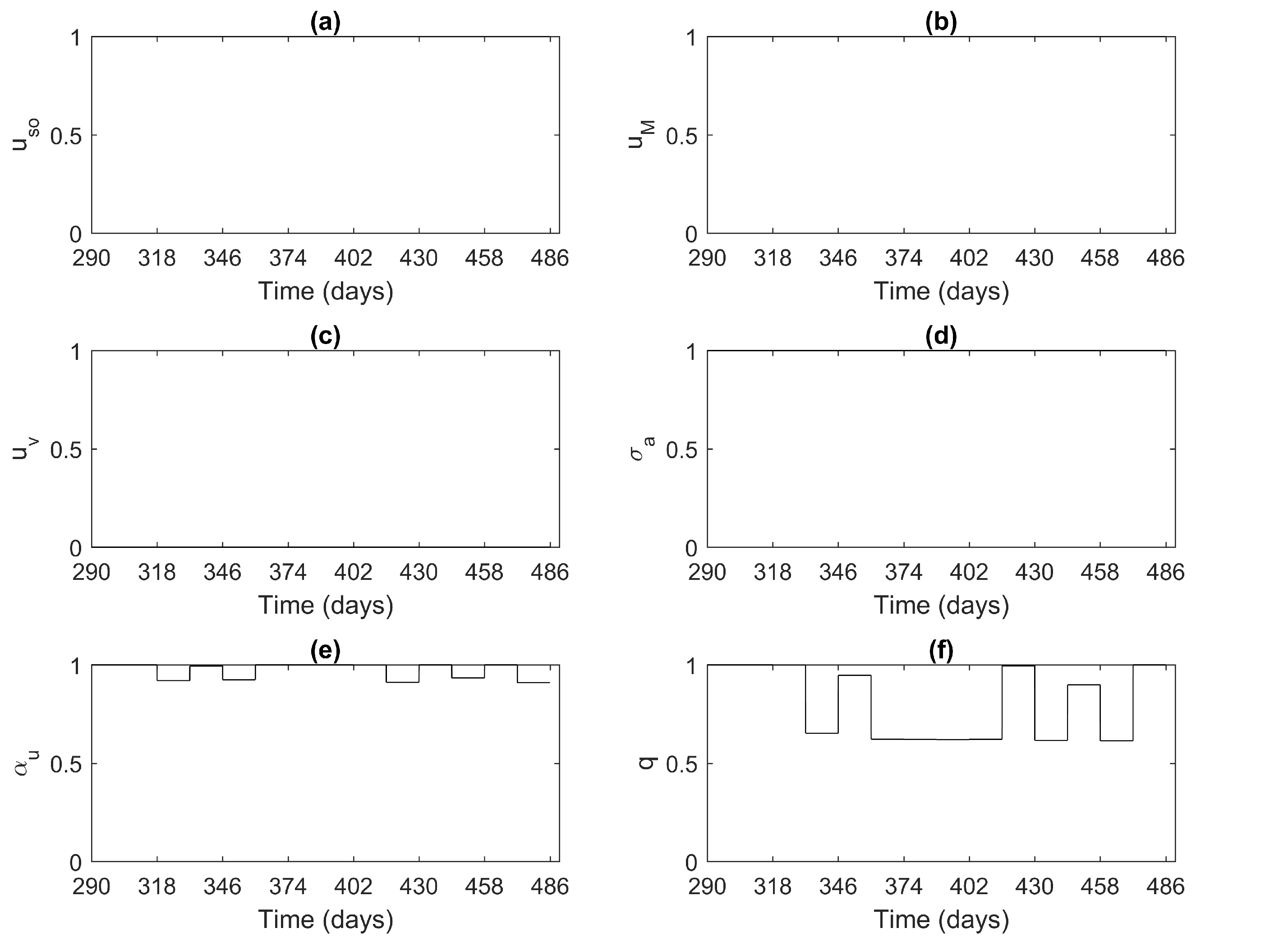
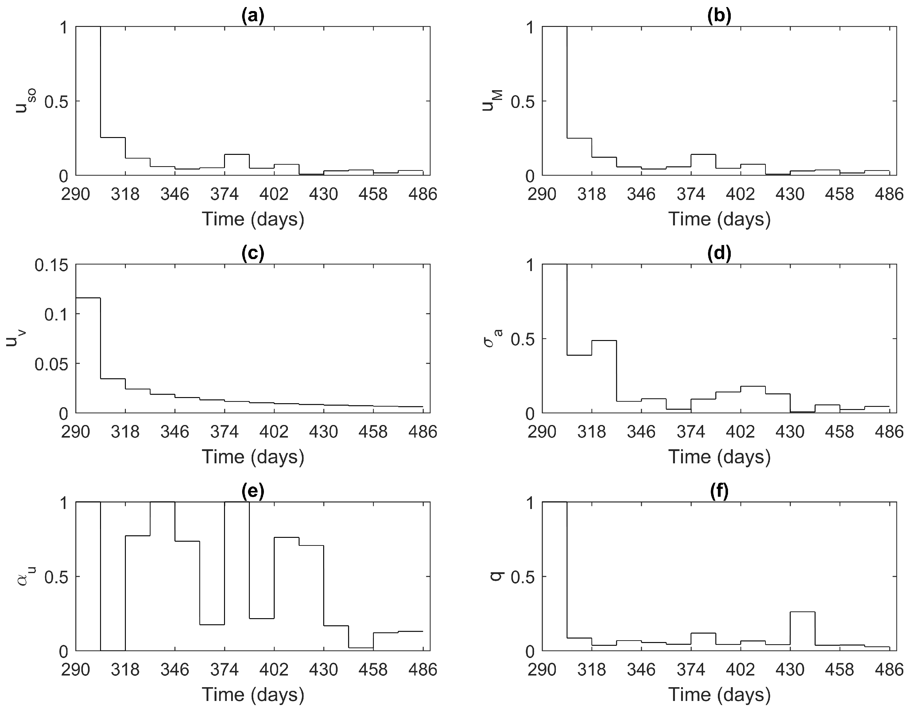
4.4. The Effectiveness of Social Isolation and Vaccination to Control the COVID-19 Pandemic

We now expect that all Thai citizens will be given immunizations to prevent the disease from spreading further. This study employed the AstraZeneca vaccine, which has a 75 percent efficacy rate and is most likely to be obtained by citizens. The number of all components in the model, except the recovery populations, is kept close to zero in Figure 8. These findings are depicted in Figure 8a,b. The numbers of populations without and under control are represented by the solid and the dashed lines, respectively. The number of sick people will drop and converge to zero as the outbreak is controlled through social isolation and vaccination policies, while the recovery populations will rise. In addition, the number of susceptible populations will decrease. The risk of infection is minimized, and people who are vaccinated will be protected from the COVID-19 pandemic.
The strategy of preventative measures, including vaccination, is shown in Figure 9. Figure 9c suggests and depicts the proportion of people who receive vaccines. As demonstrated in Figure 9a,b, the average proportion of social distancing and the use of face masks are high at first and then decrease. In Figure 9d–f, quarantine and contact tracing are also employed to prevent disease transmission from infected individuals. Moreover, a sufficient quantity of vaccinations and efficient management can improve the situation and quickly bring the pandemic under control.

5. Discussion and Conclusions

This study developed a mathematical model to describe the COVID-19 pandemic’s disease spread in Thailand. The model is built using a system of nonlinear differential equations, and it is then evaluated using model parameter estimation and real data from newly infected and death cases of the COVID-19 pandemic in Thailand. In order to determine some parameters in the model for examining disease spread in Thailand, forecasting future disease is spread to 28 weeks, and analyzing the model, the sum square error method is used to compute the model parameters. The model of the COVID-19 pandemic in Thailand is presented in (1) with the parameters in Table 1. The result of predicting the COVID-19 pandemic in Thailand shows the trend of infected populations in the model and the effectiveness of contact tracing and quarantine. After that, we propose an application of mathematical methods to plan the policy schedule for preventing disease transmission over the time horizon. To control the outbreak, model predictive control is employed to construct a scheme for isolation and vaccination measures for 28 weeks. However, reducing infections completely for all populations in a country is difficult, as it usually depends mostly on the situation in that country, including in Thailand. So, this study investigates the outbreak situation, which includes the limitation of intensive care unit capacity, social isolation without vaccination, and vaccination for a rise in herd immunity in populations.
The first scenario looked at the intensive care unit’s capacity. The number of ICU beds determines the number of patients in intensive care units, and the number of other infected people is decreasing. As a result, each week, policies were able to be relaxed. This suggests that the disease spreads based on the assumption that all patients would be admitted to an ICU service room in order to live. Following that, social isolation strategies were employed to reduce the number of sick people, which caused the number of infected people to drop to near zero. The policy plan is computed every two weeks, and it is suitable to temporarily improve the infection problem. Furthermore, the effectiveness of vaccination is evaluated in the last scenario of this work, and AstraZeneca is used as an example of a vaccine in this study. COVID-19 infection is reduced as a result of social isolation and immunization. The population that receives the vaccination will then be immune to the virus, lowering the risk of illness. The research calculated the social isolation strategy and immunization measures for each of the two weeks. As a result, if this plan can be implemented, disease transmission will be controlled within 28 weeks. As a result, the social isolation police are appropriately utilized to prevent the virus from spreading in a short period of time, but they cannot actually prevent it from spreading because it leads to subsequent difficulties, including economic problems. Vaccination is so critical in the fight against the COVID-19 pandemic.
In conclusion, this study uses mathematical modeling to investigate the COVID-19 pandemic in Thailand. Furthermore, developing preventive strategies over a long time horizon in order to minimize infection in the country depends on the circumstances that may arise. This approach impacts people who can systematically and effectively protect themselves from the virus, which is appropriate for a large group of people to apply in their real life. Furthermore, a proper plan can be implemented to decrease the waste that may result from the implementation of policies.

Author Contributions

W.S. provided the research idea, developed the mathematical model and verified the numerical results. J.J. solved the model with model predictive control to simulate the results by MATLAB programming and wrote this article. All authors have read and agreed to the published version of the manuscript.

Funding

This research was supported by the Centre of Excellence in Mathematics, Commission on Higher Education, Thailand and Faculty of Science, Mahidol University, Thailand.

Data Availability Statement

Collected data sets are publicly available in the references [11].

Conflicts of Interest

The authors declare no conflict of interest. The funders had no role in the design of the study; in the collection, analyses, or interpretation of data; in the writing of the manuscript, or in the decision to publish the results.

References

  1. Coronaviridae Study Group of the International Committee on Taxonomy of Viruses. The species Severe acute respiratory syndrome-related coronavirus: Classifying 2019-nCoV and naming it SARS-CoV-2. Nat. Microbiol. 2020, 5, 536. [Google Scholar] [CrossRef] [PubMed] [Green Version]
  2. Schwarz, L.; Tuech, J.J. Is the use of laparoscopy in a COVID-19 epidemic free of risk? Br. J. Surg. 2020, 107, e188. [Google Scholar] [CrossRef]
  3. He, X.; Cheng, X.; Feng, X.; Wan, H.; Chen, S.; Xiong, M. Clinical symptom differences between mild and severe COVID-19 patients in China: A meta-analysis. Front. Public Health 2021, 8, 954. [Google Scholar] [CrossRef] [PubMed]
  4. Ngonghala, C.N.; Iboi, E.; Eikenberry, S.; Scotch, M.; MacIntyre, C.R.; Bonds, M.H.; Gumel, A.B. Mathematical assessment of the impact of non-pharmaceutical interventions on curtailing the 2019 novel Coronavirus. Math. Biosci. 2020, 325, 108364. [Google Scholar] [CrossRef] [PubMed]
  5. Coronavirus Disease (COVID-19): How Is It Transmitted? Available online: https://www.who.int/news-room/q-a-detail/coronavirus-disease-COVID-19-how-is-it-transmitted (accessed on 14 June 2021).
  6. Li, Q.; Guan, X.; Wu, P.; Wang, X.; Zhou, L.; Tong, Y.; Ren, R.; Leung, K.S.; Lau, E.H.; Wong, J.Y.; et al. Early transmission dynamics in Wuhan, China, of novel coronavirus–infected pneumonia. N. Engl. J. Med. 2020, 382, 1199–1207. [Google Scholar] [CrossRef]
  7. WHO Coronavirus (COVID-19) Dashboard. Available online: https://covid19.who.int (accessed on 13 June 2021).
  8. COVID-19 Situation Update Worldwide, as of Week 21, Updated 10 June 2021. Available online: https://www.ecdc.europa.eu/en/geographical-distribution-2019-ncov-cases (accessed on 13 June 2021).
  9. Wu, C.P.; Adhi, F.; Culver, D. Vaccination for COVID-19: Is it important and what should you know about it? Clevel. Clin. J. Med. 2021. [Google Scholar] [CrossRef]
  10. Kaplan, R.M.; Milstein, A. Influence of a COVID-19 vaccine’s effectiveness and safety profile on vaccination acceptance. Proc. Natl. Acad. Sci. USA 2021, 118. [Google Scholar] [CrossRef]
  11. Department of Disease Control. COVID-19 Infected Situation Reports. Available online: https://ddc.moph.go.th/viralpneumonia/eng/index.php (accessed on 11 May 2021).
  12. Coronavirus Disease 2019 (COVID-19) WHO Thailand Situation Report 197-19 August 2021 [EN/TH]-Thailand. Available online: https://reliefweb.int/report/thailand/coronavirus-disease-2019-COVID-19-who-thailand-situation-report-197-19-august-2021 (accessed on 30 August 2021).
  13. COVID-19 Pandemic in Thailand. Available online: https://en.wikipedia.org/w/index.php?title=COVID-19_pandemic_in_Thailand&oldid=1028455901 (accessed on 14 June 2021).
  14. Hussain, T.; Ozair, M.; Okosun, K.O.; Ishfaq, M.; Awan, A.U.; Aslam, A. Dynamics of swine influenza model with optimal control. Adv. Differ. Equ. 2019, 2019, 508. [Google Scholar] [CrossRef]
  15. Dénes, A.; Gumel, A.B. Modeling the impact of quarantine during an outbreak of Ebola virus disease. Infect. Dis. Model. 2019, 4, 12–27. [Google Scholar] [CrossRef]
  16. Chancharoenthana, W.; Leelahavanichkul, A.; Chinpraditsuk, S.; Pongpirul, K.; Kamolratanakul, S.; Phumratanaprapin, W.; Wilairatana, P.; Pitisuttithum, P. Social restriction versus herd immunity policies in the early phase of the SARS-CoV-2 pandemic: A mathematical modelling study. Asian Pac. J. Allergy Immunol. 2021. [Google Scholar] [CrossRef]
  17. Wilasang, C.; Jitsuk, N.; Sararat, C.; Modchang, C. Reconstruction of the transmission dynamics of the first COVID-19 epidemic wave in Thailand. Res. Sq. 2021. [Google Scholar] [CrossRef]
  18. Frank, T.; Chiangga, S. SEIR order parameters and eigenvectors of the three stages of completed COVID-19 epidemics: With an illustration for Thailand January to May 2020. Phys. Biol. 2021, 18, 046002. [Google Scholar] [CrossRef] [PubMed]
  19. IHME COVID-19 Forecasting Team. Modeling COVID-19 Scenarios for the United States; Nature Publishing Group: Berlin, Germany, 2021; Volume 27, p. 94. [Google Scholar]
  20. Bastos, S.B.; Cajueiro, D.O. Modeling and forecasting the early evolution of the COVID-19 pandemic in Brazil. Sci. Rep. 2020, 10, 19457. [Google Scholar] [CrossRef]
  21. Iboi, E.; Richardson, A.; Ruffin, R.; Ingram, D.; Clark, J.; Hawkins, J.; McKinney, M.; Horne, N.; Ponder, R.; Denton, Z.; et al. Impact of public health education program on the novel coronavirus outbreak in the United States. Front. Public Health 2021, 9, 208. [Google Scholar] [CrossRef]
  22. Riyapan, P.; Shuaib, S.E.; Intarasit, A. A Mathematical Model of COVID-19 Pandemic: A Case Study of Bangkok, Thailand. Comput. Math. Methods Med. 2021, 2021, 6664483. [Google Scholar] [CrossRef]
  23. Akindeinde, S.O.; Okyere, E.; Adewumi, A.O.; Lebelo, R.S.; Fabelurin, O.O.; Moore, S.E. Caputo fractional-order SEIRP model for COVID-19 Pandemic. Alex. Eng. J. 2021, 61, 829–845. [Google Scholar] [CrossRef]
  24. Iyiola, O.; Oduro, B.; Zabilowicz, T.; Iyiola, B.; Kenes, D. System of Time Fractional Models for COVID-19: Modeling, Analysis and Solutions. Symmetry 2021, 13, 787. [Google Scholar] [CrossRef]
  25. Owusu-Mensah, I.; Akinyemi, L.; Oduro, B.; Iyiola, O.S. A fractional order approach to modeling and simulations of the novel COVID-19. Adv. Differ. Equ. 2020, 2020, 683. [Google Scholar] [CrossRef]
  26. Ndaïrou, F.; Area, I.; Nieto, J.J.; Torres, D.F. Mathematical modeling of COVID-19 transmission dynamics with a case study of Wuhan. Chaos Solitons Fractals 2020, 135, 109846. [Google Scholar] [CrossRef]
  27. Giordano, G.; Blanchini, F.; Bruno, R.; Colaneri, P.; Di Filippo, A.; Di Matteo, A.; Colaneri, M. A SIDARTHE model of COVID-19 epidemic in Italy. arXiv 2020, arXiv:2003.09861. [Google Scholar]
  28. Mahikul, W.; Chotsiri, P.; Ploddi, K.; Pan-Ngum, W. Evaluating the Impact of Intervention Strategies on the First Wave and Predicting the Second Wave of COVID-19 in Thailand: A Mathematical Modeling Study. Biology 2021, 10, 80. [Google Scholar] [CrossRef] [PubMed]
  29. Tantrakarnapa, K.; Bhopdhornangkul, B. Challenging the spread of COVID-19 in Thailand. ONE Health 2020, 11, 100173. [Google Scholar] [CrossRef] [PubMed]
  30. Giannari, A.G.; van Logtestijn, M.D.; Christodoulides, P.; Konishi, K.; Tanakal, R.J. Model predictive control for designing proactive therapy of atopic dermatitis. In Proceedings of the 2018 European Control Conference (ECC), Limassol, Cyprus, 12–15 June 2018; pp. 2387–2392. [Google Scholar]
  31. Wang, L. Model Predictive Control System Design and Implementation Using MATLAB®; Springer Science & Business Media: Berlin/Heidelberg, Germany, 2009. [Google Scholar]
  32. Maciejowski, J.M. Predictive Control: With Constraints; Pearson Education: London, UK, 2002. [Google Scholar]
  33. Yang, H.M. The basic reproduction number obtained from Jacobian and next generation matrices—A case study of dengue transmission modelling. Biosystems 2014, 126, 52–75. [Google Scholar] [CrossRef]
  34. Roberts, M.G.; Heesterbeek, J. Characterizing the next-generation matrix and basic reproduction number in ecological epidemiology. J. Math. Biol. 2013, 66, 1045–1064. [Google Scholar] [CrossRef] [PubMed] [Green Version]
  35. Singh, P.; Srivastava, S.K.; Arora, U. Stability of SEIR model of infectious diseases with human immunity. Glob. J. Pure Appl. Math. 2017, 13, 1811–1819. [Google Scholar]
  36. Tailor, M.R.; Bhathawala, P. Linearization of nonlinear differential equation by Taylor’s series expansion and use of Jacobian linearization process. Int. J. Theor. Appl. Sci. 2011, 4, 36–38. [Google Scholar]
  37. Bernal, J.L.; Andrews, N.; Gower, C.; Robertson, C.; Stowe, J.; Tessier, E.; Simmons, R.; Cottrell, S.; Roberts, R.; O’Doherty, M.; et al. Effectiveness of the Pfizer-BioNTech and Oxford-AstraZeneca vaccines on COVID-19 related symptoms, hospital admissions, and mortality in older adults in England: Test negative case-control study. BMJ 2021, 373, n1088. [Google Scholar] [CrossRef]
  38. BOI: The Board of Investment of Thailand. Available online: https://www.boi.go.th/ (accessed on 5 June 2021).
  39. Yokubol, B. Survey on Usage of Personal Protective Equipment in Known or Suspected COVID-19 Infected Patients during Anesthesia Practice in Early Pandemic 2020 in Thailand. Thai J. Anesthesiol. 2020, 46, 29–34. [Google Scholar]
  40. H Focus New. 80% of COVID-19 Cases Showing a Few Symptoms and 30% of These Groups Are Immune but Have No Symptoms. Available online: https://www.hfocus.org/content/2020/04/18886 (accessed on 11 May 2021).
  41. BANGKOKBIZ. Number of Intensive Care Unit (ICU) Beds. Available online: https://www.bangkokbiznews.com/news/detail/915139 (accessed on 11 May 2021).
Figure 1. The flow diagram showing the behavior of the COVID-19 pandemic for model (1).
Axioms 10 00274 g001
Figure 2. Curve fitting of the model parameter (1) and real data for newly infected cases (a) and death cases (b) during the second and third waves of the COVID-19 pandemic in Thailand from 1 November 2020 to 19 August 2021.
Axioms 10 00274 g002
Figure 3. The graph depicts the effectiveness of contact tracing and quarantining of people, σ a , α u , and q, on the future results of infected populations, with control in the black lines and without control in the red lines. The results with control in the graph (a) and the comparison of the results with and without control in the graph (b).
Axioms 10 00274 g003
Figure 4. Effectiveness of policy relaxations of social isolation policies for controlling the number of patients in intensive care unit when ICU bed capacity is restricted in graph (a), and the affected results of each infected individual in graph (b).
Axioms 10 00274 g004
Figure 5. The weekly schedule of social isolation policies related to ICU capacity and ICU admission. Social distancing is displayed in graph (a), the use of face mask measures in graph (b), vaccination in graph (c), contact tracing measures in graphs (d,e), and quarantine measures in graphs (f).
Axioms 10 00274 g005
Figure 6. Effectiveness of social isolation policies for the number of infected populations with control on the dash lines and without control on the solid lines, infected populations in graph (a), non-quarantine susceptible populations in graph (b) and recovery populations in graph (c).
Axioms 10 00274 g006aAxioms 10 00274 g006b
Figure 7. Figures showing the schedule of social isolation measures for each two weeks. Social distancing is displayed in graph (a), the use of face mask measures in graph (b), vaccination in graph (c), contact tracing measures in graphs (d,e), and quarantine measures in graphs (f).
Axioms 10 00274 g007
Figure 8. The effectiveness of social isolation and vaccination for infected populations in graph (a) and susceptible and recovered populations in graph (b), with the results with control in the solid lines and without control in the dashed lines.
Axioms 10 00274 g008
Figure 9. The schedule of social isolation and vaccination policies for each two weeks. Social distancing is displayed in graph (a), the use of face mask measures in graph (b), vaccination in graph (c), contact tracing measures in graphs (d,e), and quarantine measures in graphs (f).
Axioms 10 00274 g009
Table 1. The values of parameters in the model (1).
ParameterValueSourceParameterValueSource
β s o 0.9519Fitted [11] r s 1/10[4]
p0.8891Fitted [11] r i 1/8[4]
σ a 0.2533Fitted [11] r a 0.13978[4]
α u 0.0326Fitted [11] r i c u 1/10[4]
q0.0397Fitted [11] m s 0.00011Fitted [11]
ε v 0.75[37] m i 0.00011Fitted [11]
μ 0.000023[38] m a 0.5 m s [4]
N66,190,000[38] m i c u 1.5 m s [4]
Λ μ N ϕ s 1/5[4]
ψ q 1/14[4] γ 0.7[4]
σ u 1/5.2[17] v i 0.025[39]
σ q 1/5.2[17] η a 0.5[4]
δ u 0.2[40] R 0 1.23
Publisher’s Note: MDPI stays neutral with regard to jurisdictional claims in published maps and institutional affiliations.

