An Improved Tikhonov-Regularized Variable Projection Algorithm for Separable Nonlinear Least Squares

Abstract

In this work, we investigate the ill-conditioned problem of a separable, nonlinear least squares model by using the variable projection method. Based on the truncated singular value decomposition method and the Tikhonov regularization method, we propose an improved Tikhonov regularization method, which neither discards small singular values, nor treats all singular value corrections. By fitting the Mackey–Glass time series in an exponential model, we compare the three regularization methods, and the numerically simulated results indicate that the improved regularization method is more effective at reducing the mean square error of the solution and increasing the accuracy of unknowns.

1. Introduction

Many problems in physics, chemistry, machine learning, computer vision, signal processing and mechanical engineering can only be described by a specialized type of nonlinear regression model, which is a linear combination of nonlinear functions. In particular, given the sequence of the observed values $\{(t_i,y_i),i=1,2,\cdots ,m\}$, a fitting model can be established as follows:

$$\eta ({\theta }_L,{\theta }_N;t_i):={\displaystyle \sum _{j=1}^n{a}_j{\phi }_j(}{\theta }_N;t_i)$$

(1)

where ${\theta }_L={(a_1,a_2,\cdots ,a_n)}^T$ is the linear parameter, ${\theta }_N={(b_1,b_2,\cdots ,b_k)}^T$ is the nonlinear parameter and ${\phi }_j({\theta }_N;t_i)$ is a quadratic differentiable nonlinear function, which depends on ${\theta }_N$ and $t_i$. With the least squares method, it reduces to the following nonlinear function.

$$v({\theta }_L,{\theta }_N)={\displaystyle \sum _{i=1}^m(y_i-\eta ({\theta }_L,{\theta }_N;t_i)}{)}^2$$

(2)

which can be rewritten in the matrix form

$$v({\theta }_L,{\theta }_N)={\Vert y-\mathsf{\Phi }({\theta }_N){\theta }_L\Vert }^2$$

(3)

where $y={(y_1,y_2,\cdots ,y_m)}^T$, $t={(t_1,t_2,\cdots ,t_m)}^T$ and ${\varphi }_j({\theta }_N;t)=({\phi }_j({\theta }_N;t_1),\cdots {\phi }_j{({\theta }_N;t_m))}^T$. Additionally, $\mathsf{\Phi }({\theta }_N)=({\varphi }_1({\theta }_N;t),\cdots {\varphi }_n({\theta }_N;t))$ is a matrix function, and ${\Vert \cdot \Vert }^2$ denotes the Euclidean norm.

The minimization problem (3) is a nonlinear least squares problem that does not consider the properties of the parameters. The Gauss–Newton (GN) algorithm [1], the Levenberg–Marquardt (LM) algorithm [2,3] and the iterative embedding points algorithm [4] are commonly used to solve such problems. In fact, there are two sets of mutually dependent parameters in this model: the linear parameter and the nonlinear parameter. Golub and Pereyra [5,6] refer to this type of data-fitting problem as a separable nonlinear least squares (SNLLS) problem. In consideration of the specialized separable structure of this type of model, they proposed the variable projection (VP) algorithm. The general aim of implementing this algorithm is to eliminate linear parameters and obtain a simplified problem with only nonlinear parameters. For any given nonlinear parameter ${\theta }_N$, ${\theta }_L$ can be obtained by solving the following linear least squares problem.

$${\theta }_L=\arg \underset{{\theta }_L}{\min }{\Vert y-\mathsf{\Phi }({\theta }_N){\theta }_L\Vert }^2$$

(4)

The least squares solution of Equation (4) is

$${\widehat{\theta }}_L={\left(\mathsf{\Phi }{({\theta }_N)}^T\mathsf{\Phi }({\theta }_N)\right)}^{-1}\mathsf{\Phi }{({\theta }_N)}^{T}y=\mathsf{\Phi }{({\theta }_N)}^{+}y$$

(5)

where $\mathsf{\Phi }{({\theta }_N)}^{+}$ is the pseudo-inverse of $\mathsf{\Phi }({\theta }_N)$. By substituting ${\widehat{\theta }}_L$ into (3), we obtain

$$v({\theta }_N)={\Vert y-\mathsf{\Phi }({\theta }_N)\mathsf{\Phi }{({\theta }_N)}^{+}y\Vert }^2={\Vert \left(I-\mathsf{\Phi }({\theta }_N)\mathsf{\Phi }{({\theta }_N)}^{+}\right)y\Vert }^2={\Vert \left(I-P_{\mathsf{\Phi }({\theta }_N)}\right)y\Vert }^2={\Vert P_{\mathsf{\Phi }({\theta }_N)}^{\perp }y\Vert }^2$$

(6)

where $P_{\mathsf{\Phi }({\theta }_N)}=\mathsf{\Phi }({\theta }_N)\mathsf{\Phi }{({\theta }_N)}^{+}$ is the orthogonal projection on the linear space spanned by the column vectors of $\mathsf{\Phi }({\theta }_N)$, and $P_{\mathsf{\Phi }({\theta }_N)}^{\perp }=I-P_{\mathsf{\Phi }({\theta }_N)}$ is the projector on the orthogonal complement of the column space of $\mathsf{\Phi }({\theta }_N)$.

Equation (6) is the revised residual function, in which the linear parameter is eliminated. The VP algorithm reduces the dimensionality of the parameter space and increases the probability of finding the global optimal solution. It is an effective method for solving the SNLLS problem.

The VP algorithm has been significantly improved and widely applied since it was proposed. For example, Kaufman [7] proposed an improved VP algorithm based on the trapezoidal decomposition of a matrix, and provided a simplified Jacobian matrix of the VP method. Ruhe et al. [8] analyzed the asymptotic convergence of the simplified VP algorithm. O’Leary and Rust [9] subsequently discovered that a VP algorithm with a complete Jacobian matrix requires fewer iterations than Kaufman’s simplified algorithm. Alternatively, Ruano et al. [10] proposed a more simplified Jacobian matrix for the VP algorithm, and an improved VP algorithm that entailed applying QR decomposition to the sparse nonlinear function matrix. They found that their method effectively increased computational efficiency. Gan et al. [11] compared the separation algorithms for different Jacobian matrices and concluded that a VP algorithm with the complete Jacobian matrix is more stable than the simplified algorithm proposed by Kaufman. Gan and Li [12] proposed a VP algorithm that utilizes the classic Gram–Schmidt (GS) matrix decomposition method to treat cases in which the number of observations is significantly larger than the number of linear parameters; their algorithm was found to reduce the computational cost. Alternatively, Chen et al. [13] employed a modified GS method in their development of a more robust VP algorithm for SNLLS problems; they reported that the combination of a VP algorithm and the L–M method is more effective than a combination of the VP algorithm and the G–N method.

Although many considerable efforts have been dedicated to developing methods to solve SNLLS problems, there are few studies on ill-conditioned problems with iterative processes. It can be seen that the least squares solution given as Equation (5) is conditioned on the fact that ${\left(\mathsf{\Phi }{({\theta }_N)}^T\mathsf{\Phi }({\theta }_N)\right)}^{-1}\mathsf{\Phi }{({\theta }_N)}^T$ is computable—that is, the matrix $\mathsf{\Phi }{({\theta }_N)}^T\mathsf{\Phi }({\theta }_N)$ is invertible. However, when the equation is ill-conditioned, the smallest characteristic root of the matrix $\mathsf{\Phi }{({\theta }_N)}^T\mathsf{\Phi }({\theta }_N)$ is near zero; therefore, the elements of ${\left(\mathsf{\Phi }{({\theta }_N)}^T\mathsf{\Phi }({\theta }_N)\right)}^{-1}$ will become significantly large. Small changes in the observation value will significantly affect the least squares solution, causing it to become unstable. Thus, a regularization method needs to be introduced to convert the ill-posed problem into a relatively mild or benign problem [14,15,16] before proceeding. There are many regularization methods, including Tikhonov regularization (TR) [17,18], truncated singular value decomposition (TSVD) regularization [19,20], kernel-based regularization [21,22] and $l_1$-regularization [23]. Generally, a regularization method is applied to improve the condition of the ill-conditioned matrix by introducing regularization parameters. Common methods for determining regularization parameters include ridge-tracing, generalized cross-check and L-curve-based methods. The TSVD method is significantly popular because it is relatively well developed, and can be applied to solve computationally complex problems. Zeng et al. [24] estimated the linear parameters in a separable least squares parameter optimization process by implementing regularization parameter detection techniques in the TR and TSVD methods. In their attempt to regularize SNLLS ill-posed problems using a VP algorithm, Chen et al. [25] developed a weighted generalized cross-validation method to determine TR parameters. The effectiveness of the algorithm was verified through experimentation. Wang et al. [26] separated linear and nonlinear regularization parameters using a singular value decomposition (SVD)-based VP algorithm. They also estimated the linear parameters by using both the LS method and an L-curve-based spectral correction method. Their experiments confirmed that the algorithm can effectively solve ill-conditioned problems.

In this paper, an improved TR optimization method is proposed for the parameter estimation problem of SNLLS models. With the VP method as the basic framework, the algorithm was developed to take into account the specialized structure of the linear combination of nonlinear functions and separate the linear and nonlinear parameters. The linear parameters are estimated by using an improved TR method, whereas the nonlinear parameters are optimized by using the LM method. Regarding the iterative process, the simplified Jacobian matrix proposed by Kaufman is implemented in the VP algorithm. Numerical simulations were performed to compare the improved TR method to the original TR and TSVD regularization methods. The effectiveness of the VP algorithm with the improved TR method was verified, and the accuracies of different linear parameter estimation methods were evaluated.

We begin this paper by summarizing the VP method and the existing problems related to solve SNLLS problems. The methods of nonlinear parameter estimation and linear parameter estimation are explained based on an improved VP algorithm derived from SVD, and the steps to solve SNLLS problems are then detailed. Thereafter, we compare and evaluate the performances of the method proposed in this paper and the conventional regularized VP algorithm by numerical simulations.

2. Parameter Estimation Method

2.1. Regularization Algorithm for Linear Parameter Estimation

With no loss of generality, the model is abbreviated as

$$y=\mathsf{\Phi }{\theta }_L$$

(7)

Then, as a result of applying SVD, $\mathsf{\Phi }$ can be rewritten as

$$\mathsf{\Phi }=US{V}^T={\displaystyle \sum _{i=1}^l{u}_i{\sigma }_i{v}_i^T}$$

(8)

where $U=(u_1,u_2,\cdots ,u_m)$ and $V=(v_1,v_2,\cdots ,v_n)$ are composed of the eigenvectors ${\mathsf{\Phi }}^T\mathsf{\Phi }$ and $\mathsf{\Phi }{\mathsf{\Phi }}^T$ respectively; and $U\in R^{m\times m}$, $V=R^{n\times n}$, $U^{T}U=I$ and $V^{T}V=I$. $S=\mathrm{diag}({\sigma }_1,\cdots ,{\sigma }_l,{\sigma }_{l+1},\cdots ,{\sigma }_n)$ is a diagonal matrix with diagonal elements that are singular values of $\mathsf{\Phi }$, where ${\sigma }_1\ge {\sigma }_2\ge \cdots \ge {\sigma }_l>0$ and ${\sigma }_{l+1}={\sigma }_{l+2}=\cdots ={\sigma }_n=0$. $l$ is the rank of $\mathsf{\Phi }$.

The Moore–Penrose inverse of $\mathsf{\Phi }$ is given as ${\mathsf{\Phi }}^{+}={\displaystyle \sum _{i=1}^l\frac{u_i^T{v}_i}{{\sigma }_i}}$. The least squares solution of the linear parameter, according to Equation (5), is given as

$${\widehat{\theta }}_L={\displaystyle \sum _{i=1}^l\frac{u_i^{T}y{v}_i}{{\sigma }_i}}$$

(9)

Clearly, if some small singular values are significantly close to zero, even a small error will produce a significantly large discrepancy between the least square solution and the true value, making the solution unstable. To avoid this problem, a filter factor was introduced to suppress the error term in the ill-conditioned solution. Thus, the approximate solution can be obtained as

$${\widehat{\theta }}_L={\displaystyle \sum _{i=1}^l\phi \frac{u_i^{T}y{v}_i}{{\sigma }_i}}$$

(10)

2.1.1. TSVD Method

The TSVD method removes the disturbing influence of small singular values on the LS solution, thereby allowing a stable solution to be achieved. This is achieved by setting a threshold and then setting any singular value smaller than this threshold to equal zero. Generally, an appropriate threshold can be determined by setting a cutoff ratio coefficient $\alpha$, such that, if ${\sigma }_i<\alpha {\sigma }_1$, then ${\sigma }_i$ is set to zero. The corresponding TSVD filter factor is

$${\phi }_{\alpha }=\{\begin{array}{ll}1& {\sigma }_i\ge \alpha {\sigma }_1\\ 0& {\sigma }_i<\alpha {\sigma }_1\end{array}$$

(11)

At this point, the TSVD regularization solution is given as

$${\widehat{\theta }}_L={\displaystyle \sum _{i=1}^l{\phi }_{\alpha }\frac{u_i^{T}y{v}_i}{{\sigma }_i}}={\displaystyle \sum _{i=1}^k\frac{u_i^{T}y{v}_i}{{\sigma }_i}}$$

(12)

where $k\le l$ is the cutoff point for the singular value, which is typically implemented as the regularization parameter in the TSVD method.

2.1.2. TR Method

The TR method is currently the preferred method for solving ill-conditioned problems. The method entails the use of a regularization parameter $\mu$ to constrain the solution and construct a secondary optimization problem as follows:

$${\theta }_L=\arg \underset{{\theta }_L}{\min }\left\{{\Vert y-\mathsf{\Phi }({\theta }_N){\theta }_L\Vert }^2+\frac{1}{2}{\mu }^2{\Vert {\theta }_L\Vert }^2\right\}$$

(13)

where $\mu$ is the regularization parameter. When ${\theta }_N$ is fixed, the solution of Equation (13) becomes

$${\widehat{\theta }}_L={\left(\mathsf{\Phi }{({\theta }_N)}^T\mathsf{\Phi }({\theta }_N)+{\mu }^{2}I\right)}^{-1}\mathsf{\Phi }{({\theta }_N)}^{T}y$$

(14)

Subsequently, applying SVD to the matrix yields

$${\widehat{\theta }}_L={\displaystyle \sum _{i=1}^l{\phi }_{\mu }\frac{u_i^{T}y{v}_i}{{\sigma }_i}}={\displaystyle \sum _{i=1}^l\frac{{\sigma }_i^2}{{\sigma }_i^2+{\mu }^2}\frac{u_i^{T}y{v}_i}{{\sigma }_i}}$$

(15)

Thus, the TR filter factor can be expressed as ${\phi }_{\mu }=\frac{{\sigma }_i^2}{{\sigma }_i^2+{\mu }^2}$.

2.1.3. Improved TR Method

The TSVD and TR methods are essentially the same. However, there is a difference in the extent to which either method can reduce the influence of small singular values on the solution. Specifically, the TR method changes all singular values, which may cause the approximated solution to be over-smoothed. Alternatively, the TSVD method sets a small portion of the singular values to zero, which not only reduces the variance, but also affects the resolution of the solution, resulting in low accuracy. However, the improved TR method only changes small singular values by enabling the determination of the regularization matrix [27]. Given that the differences between the larger and smaller singular values of the ill-conditioned matrix are large, the singular values are determined to be small singular values with a significant influence when the sum of the standard components of small singular values accounts for more than 95% of the standard deviation. Consequently, they are regularized to reduce the influence on the standard deviation. This condition can be expressed as follows [28]:

$${\displaystyle \sum _{i=k}^l\frac{{\sigma }_0}{{\sigma }_i}}\ge 95\%{\displaystyle \sum _{i=1}^l\frac{{\sigma }_0}{{\sigma }_i}}$$

(16)

Thus, the regularization parameter $k$ can be obtained. Then, with the filter factor set as ${\phi }_{k,\mu }=\{\begin{array}{l}11<i\le k\\ \frac{{\sigma }_i^2}{{\sigma }_i^2+{\mu }^2}k<i\le l\end{array}$, when $1\le i\le k$, ${\phi }_{k,\mu }={\phi }_{\alpha }$; when $k\le i\le l$, ${\phi }_{k,\mu }={\phi }_{\mu }$. The solution of the improved TR method is

$${\widehat{\theta }}_L={\displaystyle \sum _{i=1}^l{\phi }_{k,\mu }\frac{u_i^{T}y{v}_i}{{\sigma }_i}}$$

(17)

The improved TR method is a combination of the TSVD and TR methods. Unlike the TSVD method, the improved TR method does not disregard small singular values; furthermore, it yields a more accurate solution. Additionally, unlike the conventional TR method, the improved TR method only modifies the small singular values, keeping the large singular values unchanged, to ensure high accuracy.

A regularization method is employed to determine the appropriate regularization parameters. The L-curve method was adopted in this work. This method entails selecting different $\mu$ values to obtain a set of points $\left({\Vert y-\mathsf{\Phi }{\widehat{\theta }}_L\Vert }^2,\Vert {\widehat{\theta }}_L\Vert \right)$; subsequently, an L-shaped curve is constructed with ${\Vert y-\mathsf{\Phi }{\widehat{\theta }}_L\Vert }^2$ as the abscissa and $\Vert {\widehat{\theta }}_L\Vert$ as the ordinate. Finally, the corresponding $\mu$ regularization parameter value is determined by locating the point of maximum curvature.

2.2. LM Algorithm for Nonlinear Parameter Estimation

After values for the linear parameters have been determined, Equation (6) contains only nonlinear parameters, the values of which can be determined by using the LM algorithm. The iteration strategy is

$${\theta }_N^{k+1}={\theta }_N^k+{\alpha }_k{d}_k$$

(18)

where ${\alpha }_k$ is the step length, which ensures that the objective function is in a descending state, and $d_k$ is the search direction. ${\alpha }_k$ can be obtained by employing a line search method for imprecise searches. Let $m_k$ be the smallest non-negative integer $m$ satisfying $r({\theta }_N^k+{\rho }^m{d}_k)\le r({\theta }_N^k)+\sigma {\rho }^m{g}_k^T{d}_k$ in the $k^{th}$ iteration process. Then,

$${\alpha }_k={\rho }^{m_k}$$

(19)

where $d_k$ can be determined by solving the following equation:

$$\left[J{({\theta }_N^k)}^{T}J({\theta }_N^k)+{\gamma }_{k}I\right]d_k=-J{({\theta }_N^k)}^{T}F({\theta }_N^k)$$

(20)

where ${\gamma }_k$ is the damping parameter that controls the magnitude and direction of $d_k$. When ${\gamma }_k$ is sufficiently large, the direction of $d_k$ is consistent with the negative gradient direction of the objective function. When ${\gamma }_k$ tends toward zero, $d_k$ tends toward the G–N direction. In the LM algorithm implemented here, $\gamma$ is adjusted by employing a strategy similar to adjusting the radius of the trust region [29]. A quadratic function is defined at the current iteration point as follows:

$$q(d)=r({\theta }_N^k)+{(J({\theta }_N^k)F({\theta }_N^k))}^{T}d+\frac{1}{2}{d}^T(J({\theta }_N^k)F({\theta }_N^k))d$$

(21)

The ratio of the objective function to the increment of $q(d)$ is denoted by ${\eta }_k$ as follows:

$${\eta }_k=\frac{\Delta r(d_k)}{\Delta q(d_k)}=\frac{r({\theta }_N^{k+1})-r({\theta }_N^k)}{{(J({\theta }_N^k)F({\theta }_N^k))}^T{d}_k+\frac{1}{2}{d}_k^T(J({\theta }_N^k)F({\theta }_N^k))d_k}$$

(22)

In each step of the LM algorithm, ${\gamma }_k$ is first assigned an initial value to calculate $d_k$, such as the corresponding previous iteration value. Then, ${\gamma }_k$ is adjusted according to the value of ${\eta }_k$; $d_k$ is subsequently calculated according to the adjusted ${\gamma }_k$, and a line search is performed. Clearly, when ${\eta }_k$ is close to one, $\gamma$ should be relatively smaller; this can be achieved by using the LM method to solve the nonlinear problem. When ${\eta }_k$ is close to zero, the modulus length of $d_k$ must be reduced, and $\gamma$ should be relatively larger. When ${\eta }_k$ is neither close to one nor zero, the value of the parameter ${\gamma }_k$ is determined to be suitable. The critical values of $\eta$ are typically 0.25 and 0.75. Accordingly, the update rule of ${\gamma }_k$ is given as

$${\gamma }_{k+1}:=\{\begin{array}{l}0.1{\gamma }_k,{\eta }_k>0.75,\\ {\gamma }_k,0.25\le {\eta }_k\le 0.75,\\ 10{\gamma }_k,{\eta }_k>0.25.\end{array}$$

(23)

In Equation (20), $J({\theta }_k)$ is the Jacobian matrix of the residual function, which, according to the simplified Jacobian matrix calculation method proposed by Kaufman [7], is given as

$$J_{KAU}=-P_{\mathsf{\Phi }}^{\perp }D\mathsf{\Phi }{\mathsf{\Phi }}^{-}y$$

(24)

where $D\mathsf{\Phi }$ is the Fréchet derivative of the matrix $\mathsf{\Phi }$, and ${\mathsf{\Phi }}^{-}$ is the symmetric generalized inverse of $\mathsf{\Phi }$. In [30], $P_{\mathsf{\Phi }}=\mathsf{\Phi }{\mathsf{\Phi }}^{-}$, where ${\mathsf{\Phi }}^{-}$ satisfies:

$$\mathsf{\Phi }{\mathsf{\Phi }}^{-}\mathsf{\Phi }=\mathsf{\Phi },{(\mathsf{\Phi }{\mathsf{\Phi }}^{-})}^T=\mathsf{\Phi }{\mathsf{\Phi }}^{-}$$

(25)

Thus, ${\mathsf{\Phi }}^{+}$ is not needed to calculate $P_{\mathsf{\Phi }}$.

Applying SVD to decompose matrix $\mathsf{\Phi }$ yields

$$\mathsf{\Phi }=US{V}^T=\left[U_1,U_2\right]\left[\begin{array}{cc}\mathsf{\Sigma }& 0\\ 0& 0\end{array}\right]{\left[V_1,V_2\right]}^T$$

(26)

where $\mathsf{\Sigma }$ is the $lth$ diagonal matrix, and the diagonal elements are the singular values of $\mathsf{\Phi }$. Note that $\mathrm{rank}(U_1)=\mathrm{rank}(V_1)=l$, where $l$ is the rank of $\mathsf{\Phi }$. Accordingly, we obtain

$${\mathsf{\Phi }}^{-}=\left[V_1,V_2\right]\left[\begin{array}{cc}{\mathsf{\Sigma }}^{-1}& 0\\ 0& 0\end{array}\right]{\left[U_1,U_2\right]}^T=V_1{\mathsf{\Sigma }}^{-1}{U}_1^T$$

(27)

Then

$$P_{\mathsf{\Phi }}=\mathsf{\Phi }{\mathsf{\Phi }}^{-}=\left[U_1,U_2\right]\left[\begin{array}{cc}{I}_r& 0\\ 0& 0\end{array}\right]{\left[U_1,U_2\right]}^T$$

(28)

Thus, the corresponding residual function is

$$r({\theta }_N)={\Vert P_{\mathsf{\Phi }}^{\perp }y\Vert }^2={\Vert \left[U_1,U_2\right]\left[\begin{array}{cc}0& 0\\ 0& I_{m-r}\end{array}\right]{\left[U_1,U_2\right]}^{T}y\Vert }^2={\Vert U_2{U}_2^{T}y\Vert }^2$$

(29)

and the Jacobian matrix is

$$J_{KAU}=-P_{\mathsf{\Phi }}^{\perp }D\mathsf{\Phi }{\mathsf{\Phi }}^{-}y=-U_2{U}_2^{T}D\mathsf{\Phi }{V}_1{\mathsf{\Sigma }}^{-1}{U}_1^{T}y$$

(30)

2.3. Algorithm Solution Determination

Here, we describe an improved TR optimization method for the SNLLS problem. This method entails the implementation of the VP algorithm to separate the variables, followed by the use of the improved TR method to update the linear parameters, and the LM method to search for nonlinear parameters. We compared the performance of the improved TR regularization method to those of the conventional TR method and TSVD regularization method to verify the effectiveness of the method. The model is given as

$$({\widehat{\theta }}_L,{\widehat{\theta }}_N)=\arg \left\{\underset{{\theta }_N}{\min }{\Vert y-\mathsf{\Phi }({\theta }_N){\tilde{\theta }}_L\Vert }^2,{\tilde{\theta }}_L={\displaystyle \sum _{i=1}^l\phi \frac{u_i^{T}y{v}_i}{{\sigma }_i}}\right\}$$

(31)

A summary of the steps used for obtaining the solution is given as follows:

Step 1:

Take the initial value of the nonlinear parameter ${\theta }_N^{(0)}$, the maximum number of iteration steps $M$ and set $k=0$.

Step 2:

The initial nonlinear parameter value ${\theta }_N^{(0)}$ is used to calculate the initial values of the linear parameters ${\theta }_L^{(0)}$ via the TR, TSVD or improved TR method. Then the residual function $r({\theta }_N)$ and approximate Jacobian matrix $J_{KAU}$ are obtained.

Step 3:

The iterative step length ${\alpha }_k$ and search direction $d_k$ are determined by solving Equations (19) and (20), respectively; thereafter, the nonlinear parameters are updated according to Equation (18).

Step 4:

The linear and nonlinear parameters are cross-updated until $k>M$; then, the calculation is terminated.

3. Numerical Simulation

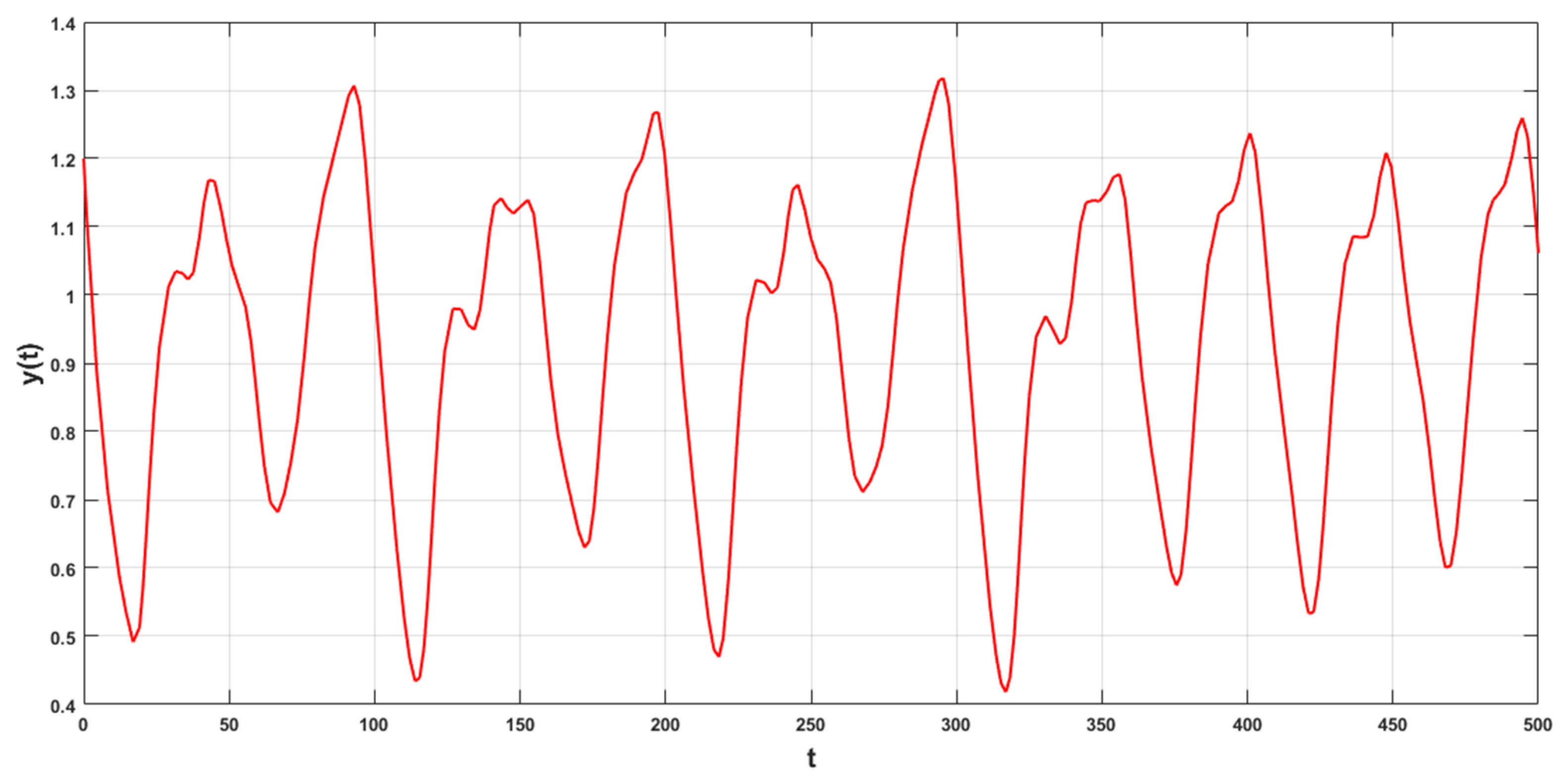
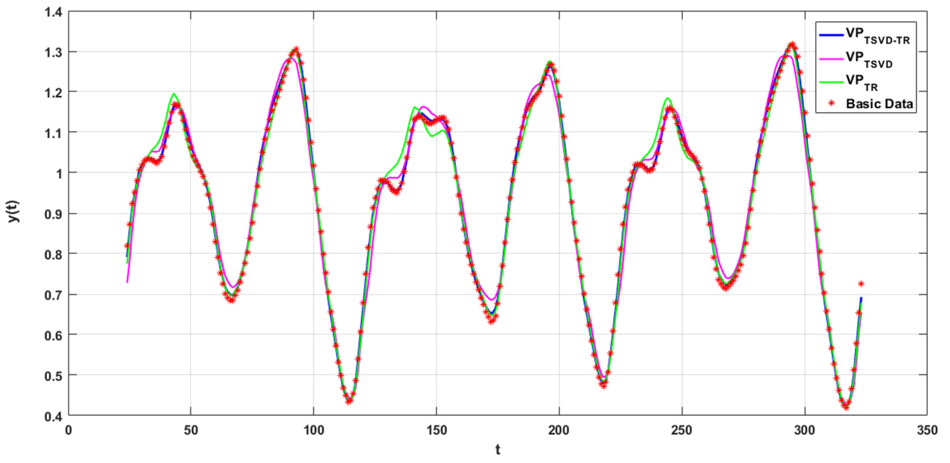
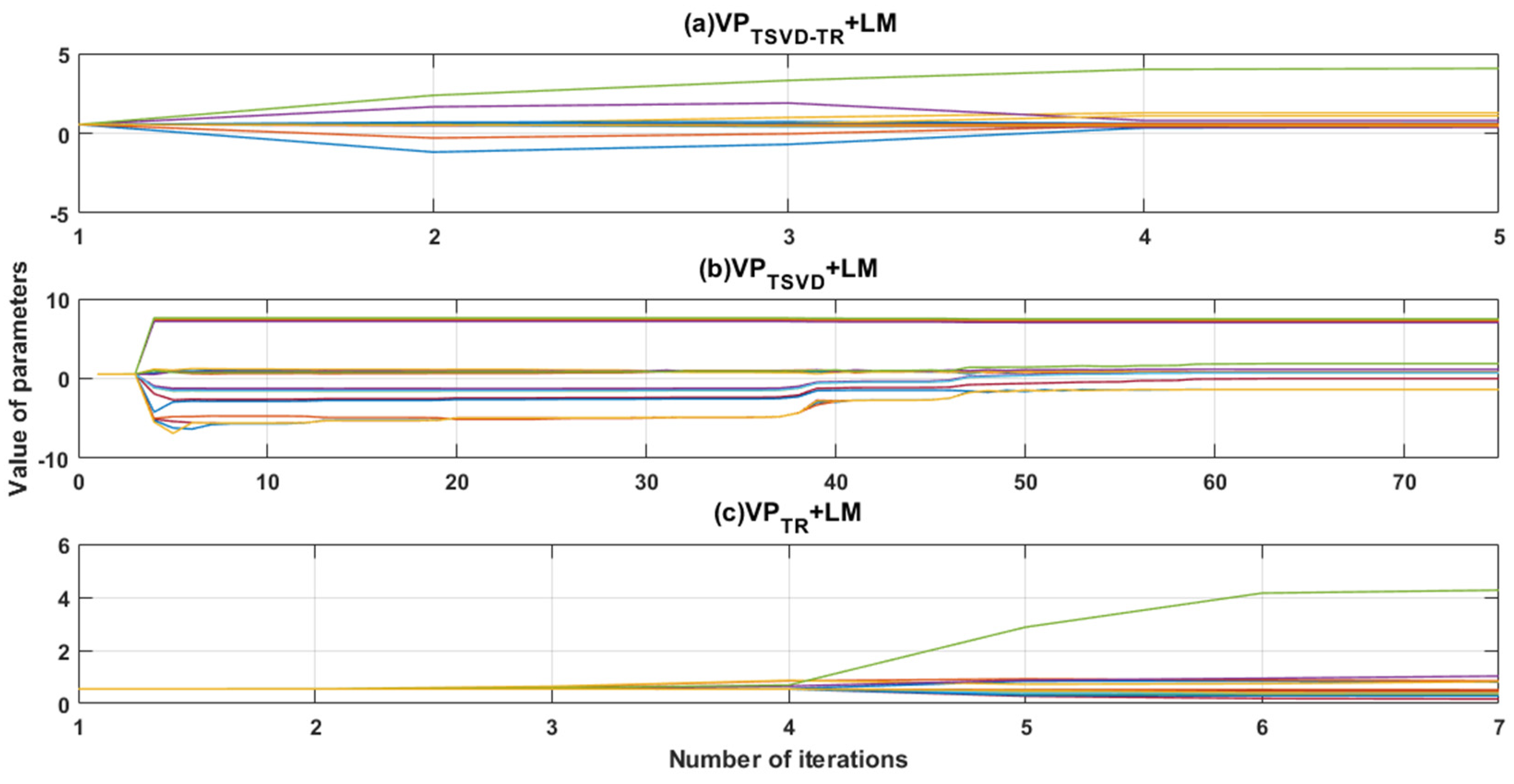
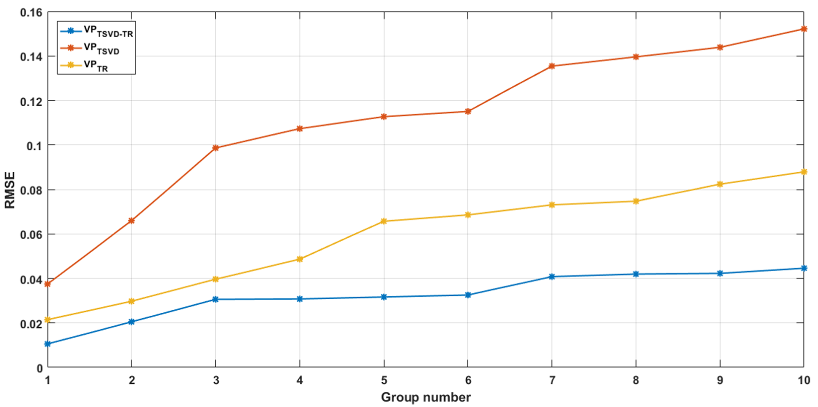
3.1. Predicting the Mackey-Class Time Series Using an RBF Neural Network

Numerical Mackey–Glass time-series simulations were performed for the validation experiment. In the experiment, the LM algorithm was separately implemented in the TSVD-based VP method (VP_TSVD), the TR-based VP method (VP_TR) and the improved TR method (VP_TSVD-TR) to fit a time-series image. This experiment was also performed to reveal the advantages and disadvantages of the aforementioned VP algorithms. The experimental environment was MATLAB R2016a running on a 1.80 GHz PC with Windows 7.

The exponential model is given as

$$\eta \left(a,\alpha ;x\right)=a_1+{\displaystyle \sum _{j=2}^n{a}_j{e}^{-{\lambda }_j{\Vert x-z_j\Vert }^2}}$$

(32)

where $a=(a_1,a_2,\cdots a_n)$ is the linear parameter set, and $\alpha ={\left({\lambda }_2,{\lambda }_3,\cdots ,{\lambda }_n;z_2^{\mathrm{T}},z_3^{\mathrm{T}},\cdots ,z_{\mathrm{n}}^{\mathrm{T}}\right)}^{\mathrm{T}}$ is the nonlinear parameter set, for the functions ${\phi }_1\left(\alpha ;x\right)\equiv 1$, ${\phi }_j\left(\alpha ;x\right)=e^{-{\lambda }_j{\Vert x-z_j\Vert }^2},$ and $j=2,3,\cdots ,n$. This model was used to fit the chaotic Mackey–Glass time series generated by the following delay differential equation:

$$\frac{dy\left(t\right)}{dt}=\frac{ay\left(t-\tau \right)}{1+y^c\left(t-\tau \right)}-by\left(t\right)$$

(33)

where $a=0.2,b=0.1,c=10,\tau =17$. The initial value condition was set as $y\left(0\right)=1.2$, and the time interval was set to 0.1. The Runge–Kutta method was used to solve the differential equation and generate 500 data points, as shown in Figure 1. Among these 500 data points, 300 were extracted from the generated data as follows:

$$\left[y\left(t-24\right),y\left(t-18\right),y\left(t-12\right),y\left(t-6\right),y\left(t\right)\right]\left(t=\left[\begin{array}{cc}24& 323\end{array}\right]\right)$$

Figure 1. Chaotic Mackey–Glass time series.

Using these 300 data points, VP_TSVD+LM, VP_TR+LM and VP_TSVD-TR+LM were applied to estimate the parameters for the model; the remaining data were used for prediction.

When n = 2, the exponential model yielded 24 nonlinear parameters and 19 linear parameters. Given the same initial iterative value, the fits of the curves derived from the training and prediction data points output by the three algorithms are shown in Figure 2. The red circles correspond to data points extracted from the time-series images. It can be intuitively determined from the figure that the curve fitted by the VP_TSVD-TR+LM algorithm is in good agreement with the data generated.

Figure 2. Curve-fitting evaluation results.

Table 1 presents the results—the number of iterations, the number of calculated functions, the second norm of the vector formed by the residuals of each point and the root mean square error (RMSE t) of the objective function with respect to the original data—for the three iterative methods. Figure 3 shows the convergences of the corresponding nonlinear parameters for the three iterative algorithms.

Table 1. Simulated results for a Mackey–Glass time series.

	Number of Iterations	Function Evaluation Number	Second Norm of Residual Vector	RMSE-t
VPTSVD	75	1953	0.34373	0.27918
VPTR	5	135	0.36427	0.19919
VPTSVD-TR	7	185	0.05818	0.09653

Figure 3. The iterative process for nonlinear parameters.

From the results in Table 1, we can see that the VP_TSVD method required the most iterations, and had the highest RMSE-t value. However, the VP_TR and the VP_TSVD-TR methods were improved significantly and optimized in the iterative process due to fewer iterations, fewer function calculations and smaller RMSEs. Although the numbers of iterations and function evaluations were similar, the results obtained by using the VP_TSVD-TR method to calculate the model parameters were considerably more accurate.

From Figure 3, it is evident that all three methods yielded converging results with the same initial values. However, the results of the VP_TSVD+LM method began to approach the optimized solution around the 40th iteration, whereas the VP_TSVD-TR+LM algorithm began slowly approaching the optimized parameter values at the third iteration, indicating a higher rate of convergence.

Every 10 points were grouped, beginning at the 400th point in the Mackey–Glass time series, to obtain several time-series predictions. The RMSE results for each group are shown in Figure 4.

Figure 4. RMSE results following multi-step time-series forecasting.

It can be seen from Figure 4 that the RMSE values for the VP_TSVD+LM method increased with the number of predictions, indicating decreasing prediction accuracy and degrading prediction ability. Conversely, in the case of the VP_TSVD-TR+LM method, there was a minimal increase in the RMSE, proving the superior stability of the method. These results also indicate that the proposed method features a higher prediction accuracy.

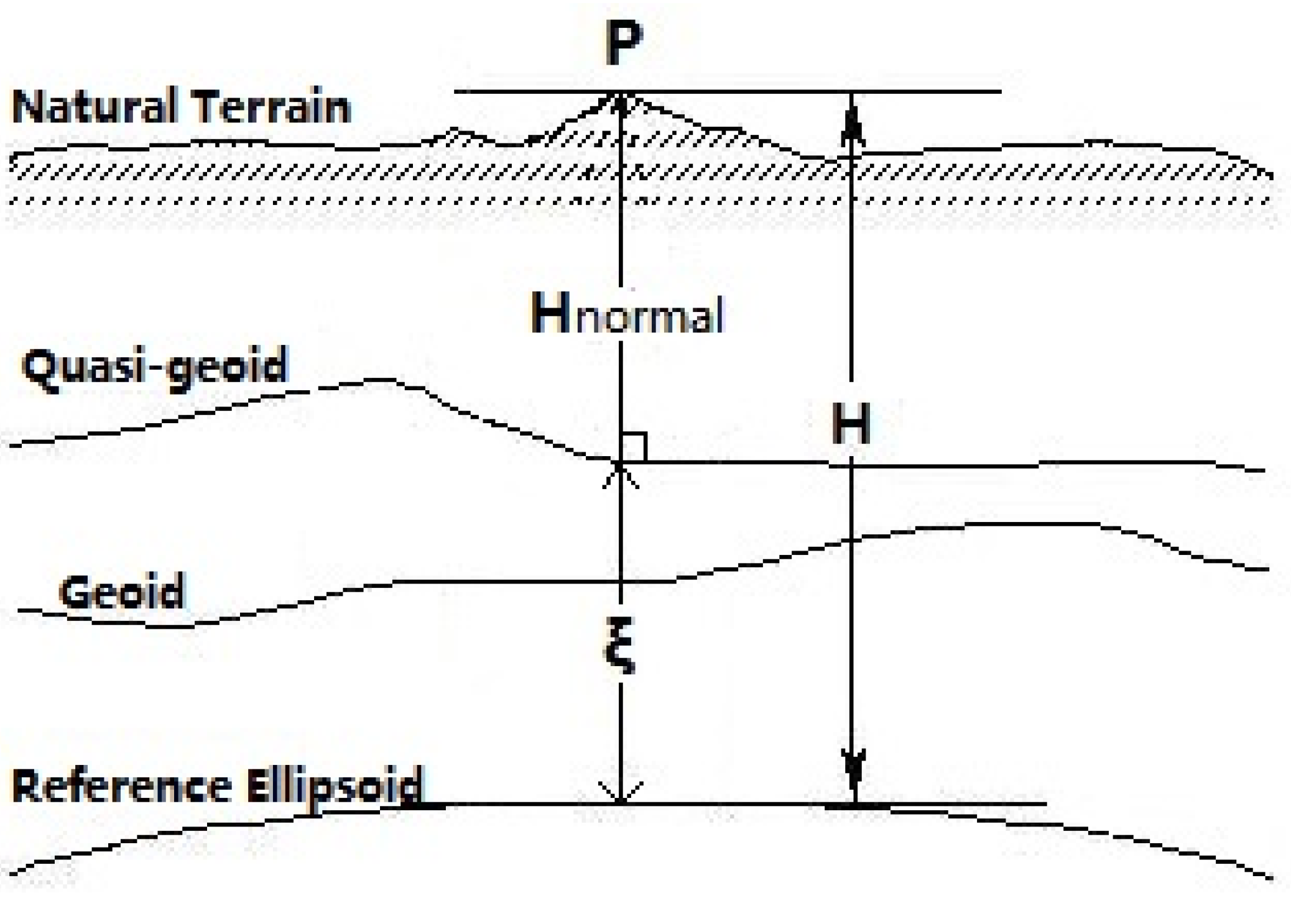
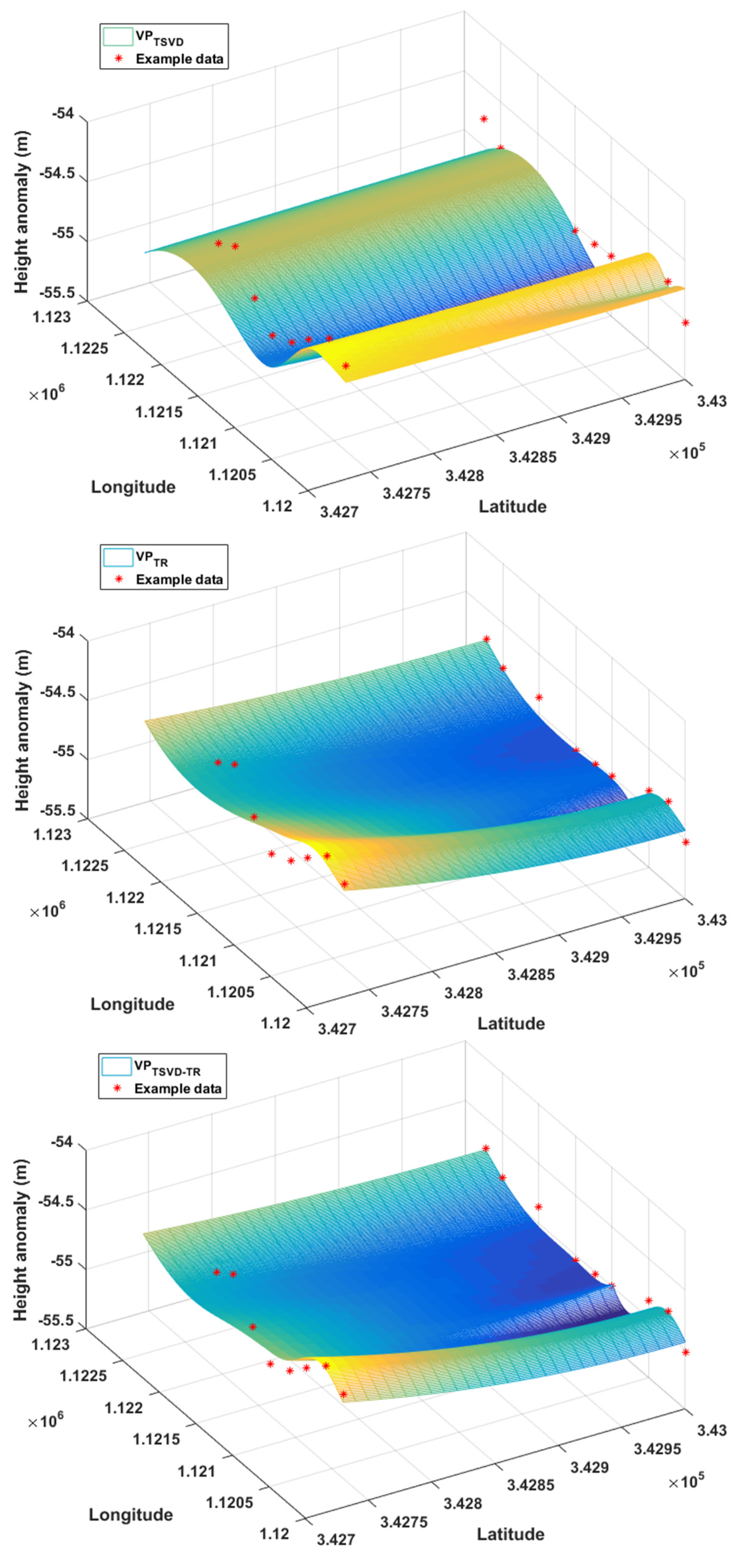
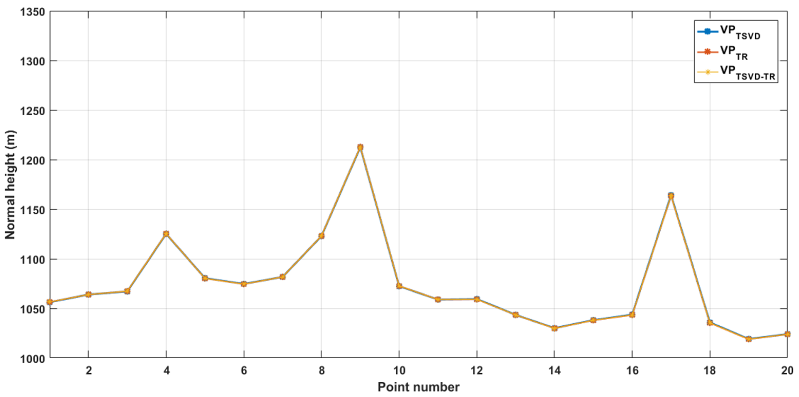
3.2. Height Anomaly Fitting

A height anomaly is the difference in elevation between the surface of the reference ellipsoid and a quasi-geoid. As we can see in Figure 5, the height anomaly $\xi$ can be expressed as $\xi =H-H_{normal}$. The geodetic height of a point can be calculated by the GPS positioning technique. The normal height can be calculated as long as the height anomaly is determined in the certain area.

Figure 5. A geodetic height, normal height and height anomaly.

A multi-surface function model was used, and its expression had the characteristic that the linear and nonlinear parameters could be separated. The TSVD method, TR method and improved algorithm were applied to solve the parameters of the model according to the height anomaly values of known control points. The model is best expressed as:

$${\xi }_i={\displaystyle \sum _{i=1}^n{a}_i{Q}_i}(X,Y,X_i,Y_i)$$

(34)

where $Q_i(X,Y,X_i,Y_i)=\sqrt{{(X-X_i)}^2+{(Y-Y_i)}^2+b_i^2}$. The example data, coordinates, geodetic heights, normal heights and height anomaly values of the known points are shown in Table 2.

Table 2. Coordinates, geodetic heights ($H$), normal heights ($H_{normal}$) and height anomaly values ($\xi$).

No.	Latitude	Longitude	$\mathit{H}\left(\mathbf{m}\right)$	${\mathit{H}}_{\mathit{n}\mathit{o}\mathit{r}\mathit{m}\mathit{a}\mathit{l}}\left(\mathbf{m}\right)$	$\mathit{\xi }\left(\mathbf{m}\right)$
D01	343000.0000	1120000.0000	1001.5220	1056.5490	−55.0270
D02	343000.0000	1120230.0000	1009.1290	1063.9280	−54.7990
D03	343000.0000	1120500.0000	1012.3950	1067.2510	−54.8560
D04	343000.0000	1120730.0000	1070.1860	1125.3030	−55.1170
D05	343000.0000	1121000.0000	1025.2330	1080.2320	−54.9990
D06	343000.0000	1121230.0000	1019.4310	1074.4540	−55.0230
D07	343000.0000	1121500.0000	1026.7090	1081.7560	−55.0470
D08	343000.0000	1121730.0000	1067.9940	1123.1420	−55.1480
D09	343000.0000	1122000.0000	1157.7220	1212.5890	−54.8670
D10	343000.0000	1122230.0000	1017.5320	1072.6350	−55.1030
D11	343000.0000	1122500.0000	1004.0630	1058.9510	−54.8880
D12	343000.0000	1122730.0000	1004.3500	1059.1140	−54.7640
D13	342730.0000	1120000.0000	988.8130	1043.3570	−54.5440
D14	342730.0000	1120230.0000	975.3010	1029.7370	−54.4360
D15	342730.0000	1120500.0000	983.5130	1038.1040	−54.5910
D16	342730.0000	1120730.0000	988.8550	1043.5930	−54.7380
D17	342730.0000	1121000.0000	1108.9430	1163.7680	−54.8250
D18	342730.0000	1121230.0000	980.5940	1035.2260	−54.6320
D19	342730.0000	1121500.0000	964.1870	1018.5260	−54.3390
D20	342730.0000	1120000.0000	1001.5220	1056.5490	−55.0270

D01–D15 were used for fitting, and the rest were used to verify the reliability of the parameters and the prediction abilities of the three algorithms. The iteration initial values of the nonlinear parameters were set to 0.5. Model (34) and the algorithm proposed in this paper were applied to fit the height anomalies, and the results are compared with the results calculated by VP_TSVD and VP_TR.

The parameter estimations were obtained after alternative calculations between the linear parameters and nonlinear parameters. The fitting images corresponding to the three algorithms are shown in Figure 6. Table 3 shows the residual sum of squares, root mean squared error and coefficient of determination values during the processes of fitting and prediction. It can be concluded from Table 3 that all algorithms enabled the model to get high fitting accuracy. During fitting and prediction, The order of magnitude of the root mean square error for VP_TSVD, VP_TR and VP_TSVD-TR is respectively 10⁻¹, 10⁻² and 10⁻³. The accuracy of VP_TSVD algorithm was slightly lower. The fitting accuracies of VP_TR and VP_TSVD-TR were higher. It can be seen from SSR_f and RMSE_f that the improved algorithm proposed in this paper had better performance in height anomaly prediction.

Figure 6. Fitting effects with respect to height anomaly values.

Table 3. Residual sum of squares (SSR, SSR_f), root mean squared error (RMSE, RMSE_f) and coefficient of determination ($R^2$) values.

Algorithms	SSR (m2)	SSRf (m2)	RMSE (m)	RMSEf (m)	${\mathit{R}}^2$
VPTSVD	0.5004	0.9337	0.1826	0.4321	0.2599
VPTR	0.0850	0.3770	0.0753	0.2746	0.8744
VPTSVD-TR	0.0798	0.3545	0.0729	0.2663	0.8820

The normal height of each point was obtained according to $H_{normal}=H-\xi$ and the height anomaly values fitted by three variable projection algorithms. The parameter estimations were verified by the known normal height. Figure 7 shows the fitting effects, and Table 4 lists the normal height fitting residual and RMSE of each point. It can be concluded from Figure 7 and Table 4 that the differences between the normal heights estimated by the three algorithms and the known example data are very small, and the three broken lines are almost coincident, which indicates that the model well fit the normal heights of known points. This is consistent with the conclusions drawn in Figure 6 and Table 3.

Figure 7. Normal height fitting effects.

Table 4. Fitting residuals (r) and RMSEs of the normal heights.

No.	Hnormal (m)	rTSVD (m)	rTR (m)	rTSVD+TR (m)
D01	1056.5490	0.2871	0.1041	0.0902
D02	1063.9280	−0.0457	−0.0457	−0.0161
D03	1067.2510	0.1498	−0.0245	−0.0742
D04	1125.3030	0.1702	0.0015	0.0224
D05	1080.2320	−0.2271	−0.0266	0.0108
D06	1074.4540	−0.1912	−0.0084	−0.0399
D07	1081.7560	−0.0025	−0.0036	−0.0052
D08	1123.1420	0.2312	0.0942	0.1011
D09	1212.5890	0.0406	−0.1688	−0.1694
D10	1072.6350	0.2850	0.1092	0.1078
D11	1058.9510	−0.0049	−0.0108	−0.0069
D12	1059.1140	−0.2656	−0.0069	−0.0091
D13	1043.3570	−0.1411	−0.0576	−0.0701
D14	1029.7370	−0.2104	−0.0699	−0.0269
D15	1038.1040	−0.0726	0.1139	0.0854
D16	1043.5930	−0.1204	0.1882	0.0878
D17	1163.7680	−0.2611	0.2026	0.1069
D18	1035.2260	−0.4721	−0.0523	−0.1058
D19	1018.5260	−0.6528	−0.4140	−0.4319
D20	1056.5490	−0.4494	−0.3555	−0.3710
RMSE	0	0.2678	0.1520	0.1474

4. Conclusions

Separable nonlinear models have been widely applied in many fields and studied by many scholars all over the world. The VP method is one of the most effective algorithms for solving related problems. However, the classical VP method may not be able to estimate the parameters of ill-conditioned problems. As regularization is the most common method for solving ill-conditioned problems, we proposed an improved regularized VP method for the SNLLS problem. This method entails applying certain rules to determine the filter factors necessary to correct small singular values, and using the L-curve method to determine regularization parameters. The results of numerical simulations revealed that the mean square error of the proposed regularized VP method was less than those of the TSVD and TR methods. Furthermore, we found that combining a regularization method with the LM algorithm-based nonlinear parameter estimation method results in a higher rate of convergence. This improved regularized parameter estimation method was demonstrated to have certain advantages in terms of its ability to mitigate the ill-conditioned problem and improve parameter estimation accuracy. It was also found to be more stable when applied to an SNLLS problem.

References

- Okatani, T.; Deguchi, K. On the Wiberg algorithm for matrix factorization in the presence of missing components. Int. J. Comput. Vis. 2007, 72, 329–337. [Google Scholar] [CrossRef]
- Levenberg, K. A method for the solution of certain non-linear problems in least squares. Q. Appl. Math. 1944, 2, 164–168. [Google Scholar] [CrossRef]
- Marquardt, D.W. An Algorithm for Least-Squares Estimation of Nonlinear Parameters. SIAM J. Appl. Math. 1963, 11, 431–441. [Google Scholar] [CrossRef]
- Hong, J.H.; Zach, C.; Fitzgibbon, A. Revisiting the variable projection method for separable nonlinear least squares problems. In Proceedings of the 2017 IEEE Conference on Computer Vision and Pattern Recognition (CVPR), Honolulu, HI, USA, 21–26 July 2017; pp. 5939–5947. [Google Scholar]
- Golub, G.H.; Pereyra, V. The Differentiation of Pseudo-Inverses and Nonlinear Least Squares Problems Whose Variables Separate. SIAM J. Numer. Anal. 1973, 10, 413–432. [Google Scholar] [CrossRef]
- Golub, G.H.; Pereyra, V. Separable nonlinear least squares: The variable projection method and its applications. Speech Commun. 2003, 45, 63–87. [Google Scholar] [CrossRef]
- Kaufman, L. A variable projection method for solving separable nonlinear least squares problems. BIT Numer. Math. 1975, 15, 49–57. [Google Scholar] [CrossRef]
- Ruhe, A. Algorithms for separable nonlinear least squares problems. SIAM Rev. 1980, 22, 318–337. [Google Scholar] [CrossRef]
- O’Leary, D.P.; Rust, B.W. Variable projection for nonlinear least squares problems. Comput. Optim. Appl. 2013, 54, 579–593. [Google Scholar] [CrossRef]
- Ruano, A.E.B.; Jones, D.I.; Fleming, P.J. A new formulation of the learning problem of a neural network controller. In Proceedings of the 30th IEEE Conference on Decision and Control, Brighton, UK, 11–13 December 1991; pp. 865–866. [Google Scholar]
- Gan, M.; Chen, C.L.P.; Chen, G.; Chen, L. On some separated algorithms for separable nonlinear least squares problems. IEEE Trans. Cybern. 2018, 48, 2866–2874. [Google Scholar] [CrossRef]
- Gan, M.; Li, H. An Efficient Variable Projection Formulation for Separable Nonlinear Least Squares Problems. IEEE Trans. Cybern. 2014, 44, 707–711. [Google Scholar] [CrossRef]
- Chen, G.Y.; Gan, M.; Ding, F. Modified Gram-Schmidt Method Based Variable Projection Algorithm for Separable Nonlinear models. IEEE Trans. Neural Netw. Learn. Syst. 2019, 30, 2410–2418. [Google Scholar] [CrossRef]
- Böckmann, C. A modification of the trust-region Gauss-Newton method to solve separable nonlinear least squares problems. J. Math. Syst. Estim. Control 1995, 5, 1–16. [Google Scholar]
- Chung, J.J.; Nagy, G. An efficient iterative approach for large-scale separable nonlinear inverse problems. SIAM J. Sci. Comput. 2010, 31, 4654–4674. [Google Scholar] [CrossRef]
- Li, X.L.; Liu, K.; Dong, Y.S.; Tao, D.C. Patch alignment manifold matting. IEEE Trans. Neural Netw. Learn. Syst. 2018, 29, 3214–3226. [Google Scholar] [CrossRef]
- Tikhonov, A.N.; Arsenin, V.Y. Solutions of ill-posed problems. SIAM Rev. 1979, 21, 266–267. [Google Scholar]
- Park, Y.; Reichel, L.; Rodriguez, G. Parameter determination for Tikhonov regularization problems in general form. J. Comput. Appl. Math. 2018, 343, 12–25. [Google Scholar] [CrossRef]
- Hansen, P.C. The Truncated SVD as A Method for Regularization. BIT Numer. Math. 1987, 27, 534–553. [Google Scholar] [CrossRef]
- Xu, P.L. Truncated SVD methods for Discrete Linear Ill-posed Problems. Geophys. J. Int. 1998, 1335, 505–514. [Google Scholar] [CrossRef]
- Aravkin, A.Y.; Drusvyatskiy, D.; van Leeuwen, T. Efficient quadratic penalization through the partial minimization technique. IEEE Trans. Autom. Control 2018, 63, 2131–2138. [Google Scholar] [CrossRef]
- Pang, S.C.; Li, T.; Dai, F.; Yu, M. Particle Swarm Optimization Algorithm for Multi-Salesman Problem with Time and Capacity Constraints. Appl. Math. Inf. Sci. 2013, 7, 2439–2444. [Google Scholar] [CrossRef][Green Version]
- Wang, X.Z.; Liu, D.Y.; Zhang, Q.Y.; Huang, H.L. The iteration by correcting characteristic value and its application in surveying data processing. J. Heilongjiang Inst. Technol. 2001, 15, 3–6. [Google Scholar]
- Zeng, X.Y.; Peng, H.; Zhou, F.; Xi, Y.H. Implementation of regularization for separable nonlinear least squares problems. Appl. Soft Comput. 2017, 60, 397–406. [Google Scholar] [CrossRef]
- Chen, G.Y.; Gan, M.; Chen CL, P.; Li, H.X. A Regularized Variable Projection Algorithm for Separable Nonlinear Least–Squares Problems. IEEE Trans. Autom. Control 2019, 64, 526–537. [Google Scholar] [CrossRef]
- Wang, K.; Liu, G.L.; Tao, Q.X.; Zhai, M. Efficient Parameters Estimation Method for the Separable Nonlinear Least Squares Problem. Complexity 2020, 2020, 9619427. [Google Scholar] [CrossRef]
- Fuhry, M.; Reichel, L. A new Tikhonov regularization method. Number Algorithms 2012, 59, 433–445. [Google Scholar] [CrossRef]
- Lin, D.f.; Zhu, J.j.; Song, Y.C. Regularized singular value decomposition parameter construction method. J. Surv. Mapp. 2016, 45, 883–889. [Google Scholar]
- Byrd, R.H.; Schnabel, R.B.; Shultz, G.A. A Trust Region Algorithm for Nonlinearly Constrained Optimization. SIAM J. Numer. Anal. 1987, 24, 1152–1170. [Google Scholar] [CrossRef]
- Golub, G.H.; Styan, G.P.H. Numerical computations for univariate linear models. J. Stat. Comput. Simul. 1973, 2, 253–274. [Google Scholar] [CrossRef]
Publisher’s Note: MDPI stays neutral with regard to jurisdictional claims in published maps and institutional affiliations. |
© 2021 by the authors. Licensee MDPI, Basel, Switzerland. This article is an open access article distributed under the terms and conditions of the Creative Commons Attribution (CC BY) license (https://creativecommons.org/licenses/by/4.0/).