Prediction of Ore Production in a Limestone Underground Mine by Combining Machine Learning and Discrete Event Simulation Techniques

Abstract

This study proposes a novel approach for enhancing the productivity of mining haulage systems by developing a hybrid model that combines machine learning (ML) and discrete event simulation (DES) techniques to predict ore production. This study utilized time data collected from a limestone underground mine using tablet computers and Bluetooth beacons for 15 weeks. The collected data were used to train an ML model to predict truck cycle time, and the support vector regression with particle swarm optimization (PSO–SVM) model demonstrated the best performance. The PSO–SVM model accurately predicted cycle time with a mean absolute error (MAE) of 2.79 min, mean squared error (MSE) of 14.29 min², root mean square error (RMSE) of 3.79 min, and coefficient of determination (R²) of 0.68. The output of the ML model was linked to the DES model to predict ore production for each truck, section, and time period. Verification of the DES model demonstrated its ability to accurately simulate the haulage system in the study area by comparing production logs with the simulation results. This study’s novel approach offers a new method for predicting ore production and determining the optimal equipment combination for each workplace, thus enhancing productivity in mining haulage systems.

1. Introduction

Mining ore from the mine and transporting it to a mineral processing plant consists of unit tasks including drilling, blasting, loading, and transportation. The profitability of a mine may depend on the operation of its production process. In particular, as the haulage costs of ore and waste account for more than half of mine operating costs, it is very important to operate the mine haulage system efficiently [1,2,3,4]. Therefore, it is necessary to establish an optimal operation and equipment utilization plan that can maximize mine productivity and minimize operating costs [5,6,7,8,9].

Ore production is the most important performance indicator for mining haulage systems, and various studies have been conducted to predict production and to optimize haulage systems. Since Rist [10] first implemented discrete event simulation (DES) in 1961, studies from the perspective of system science have been actively conducted to predict and optimize production by developing a simulation model for simulating mining haulage systems. Many researchers have set up simulation scenarios according to operating conditions, such as operation time, number of equipment units, equipment dispatch interval, and time required for unit operation, and then conducted simulations. Thus, indicators related to the productivity of mine haulage systems have been predicted [5,7,11,12,13,14,15,16,17,18,19,20,21,22,23,24]. Torkamani and Askari-Nasab [25] developed a simulation model that can analyze a transport system consisting of trucks and shovels in relation to the establishment of short-term mine planning and presented a methodology to implement it. Salama and Greberg [26] implemented a mine haulage system consisting of three load-haul-dump (LHD) machines and three trucks using SimMine simulation software and evaluated the effect of the increase in the size and number of equipment units on the production of the mine. Ozdemir and Kumral [27] used a simulation technique to improve the efficiency of haulage systems by proposing a real-time truck dispatch method using a mathematical optimization method. Park and Choi developed GPSS/H-based programs and user-friendly programs to simulate truck-loader transport systems, taking into account various conditions, such as fixed- and real-time truck dispatch, crusher capacity, and truck failure [28,29,30,31,32,33]. The input data of the DES model include factors for simulation operation, time-related factors, and factors for economic analysis. In particular, time-related factors include the time required for unit operations related to truck cycle time theory, equipment failure and repair, and equipment dispatch intervals. It is a very difficult task to measure or collect the time required for unit operations over a long period of time at an actual mine site. Therefore, most of the simulation models that have been developed so far use statistical values of time data collected for a short period of time as input data. In addition, studies have been conducted to examine methods and possibilities of predicting productivity indicators in consideration of various cases.

Recently, attempts have been made to solve production prediction problems and to optimize systems from the perspective of data science using data from mines collected in real time using smart technology. In particular, large amounts of data have been collected in real time by applying Internet of Things (IoT) and smart sensor technologies to mines, and research is actively being conducted on machine learning (ML) models to predict production and to optimize systems. Soofastaei et al. [34] estimated parameters related to production (load and truck speed) to reduce fuel consumption in haulage systems using artificial neural networks (ANNs) and genetic algorithms (GAs). Baek and Choi [35] suggested a new method for predicting crusher utilization rates and ore production of underground mine truck haulage systems using a deep neural network (DNN) model as an ML technology for the development and operation of mineral resources. Baek and Choi [36] analyzed the operating conditions in an open-pit mine and used a DNN model to estimate the amount of ore production. Choi et al. [37] developed and evaluated various ML algorithms for learning data collected using IoT systems to estimate ore production in an open-pit mine. ML models can be used to predict productivity metrics for mine haulage systems using data that can be gathered from mine sites. Therefore, assuming that the operating conditions and methods for the haulage system will not change, the latest productivity indicators can be predicted by simply inputting additionally collected data into the developed prediction model. In other words, there is an advantage in that the developed prediction model can be continuously updated and used throughout the life of the mine.

As described above, DES and ML techniques are actively used to predict and optimize mine production. However, both of these approaches have clear advantages and disadvantages. Although a DES model based on the domain knowledge of a mine can be widely used in consideration of various operating conditions in the field, it is difficult to sufficiently verify the accuracy of the prediction results. In contrast, the ML model learns based on actual field data and shows high prediction accuracy, but the prediction accuracy rapidly decreases when operation methods, such as equipment and haulage routes in the field, change and/or fall out of the operating range of the data collected in the past. Therefore, recently, studies have been conducted to establish control strategies for mining systems using both DES and ML techniques. Peña-Graf et al. [38] proposed a framework combining DES and ML to integrate decision-making processes considering geological uncertainty and used it to assess and mitigate potential risks to gold mineral processing performance. Wilson et al. [39] evaluated a system for geological uncertainty by integrating DES with data generated by partial least squares (PLS) regression. In addition, Wilson et al. [40] developed a framework combining ANNs and DES for the regional coordination of refractory gold ores to be processed in a centralized plant. However, the aim of the DES technique in these studies is to simulate ML-enabled control strategies. There is still a lack of research using DES techniques as part of the control strategy.

This study presents a new model combining the advantages of DES and ML approaches to predict the production of a mine haulage system and to derive an optimal operation plan. To this end, a limestone mine located in Korea was chosen as the research area, and truck operation time data of the underground mine were collected using Bluetooth beacons and tablet PCs. An ML model was developed to predict the truck cycle time based on recorded data. The results from predicting ore production by time period were calculated and presented by linking the predicted cycle time with the DES model.

2. Research Area and Data Collection

2.1. Research Area

Seongshin Minefield Co. (37°1712″ N, 128°4353″ E) in South Korea was selected as the research area, and an ML–DES hybrid model was developed to predict the truck cycle time and ore production of a mine haulage system using truck operation time data collected in the research area (Figure 1). The mine produces approximately 4500 metric tons of limestone per day by applying the room and pillar method. Ore production takes place 8 h a day, excluding lunch breaks (1 h). The mined limestone is loaded into a truck by a loader and transported to the processing plant after being classified by grade. Table 1 shows the types and number of equipment units used to load and transport ore or waste in the study area. In the study area, 3 loaders (with bucket sizes of 4.76 to 5.70) and 10 trucks (with loading capacities of 23 and 37 metric tons) are used to produce the limestone ore. In addition, the mine operates 8 loading points with different ore grades and 3 dumping points (crushers). The production manager establishes a daily production plan considering the daily target of ore production and grade. After establishing the daily production plan, the manager dispatches loaders and trucks to three loading points. The trucks move to the loading point, load the ore, and haul it to the processing plant. The trucks that have dumped the ore move back to the loading point and repeat the ore hauling operation.

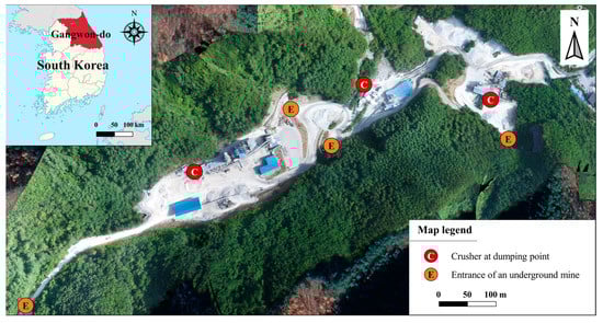
Figure 1. Aerial view of research area.

Table 1. Description of datasets for training machine learning model.

Equipment	Capacity	Amount
Loaders	4.76 m3	1
	5.00 m3	1
	5.70 m3	1
Trucks	23.0 ton	7
	37.5 ton	3

2.2. Data

2.2.1. Method for Data Collection

Bluetooth beacons and tablet PCs (short-range wireless communication devices) were used to collect log data on the travel time of trucks used in the mine haulage system in the research area. A Bluetooth beacon periodically transmits user information (ID) as a Bluetooth signal. When a user with a tablet PC enters the signal reach area, the smartphone app receives a Bluetooth signal and delivers an ID to a server, which recognizes the individual and transmits related information to the user’s tablet PC to provide Bluetooth beacon-based services. In this study, an indoor positioning system among various services provided by Bluetooth beacons was used to collect log data on the travel times of trucks used in the mine haulage system. Bluetooth beacons were installed on the main haulage route where trucks travel in the mine haulage system, and the passing time of a truck was recorded when a truck with a tablet PC passed through the location in which the Bluetooth beacon was installed. The Bluetooth beacons were installed at the main locations along the haulage route (loading point, junction, etc.), at the crusher (dumping point), and on the loaders (Figure 2). A total of 22 beacons were installed on the haulage route (11 beacons) and the loading points (8 beacons) and dumping points (3 beacons), and beacons were installed on 3 loaders used in the mine transport system. The beacons installed on the haulage route and the crusher were fixed to the wall of the tunnel or structure, and the beacons installed on the loader were attached to the windshield or room mirror of the truck’s cabin. The average temperature and precipitation data of the research area used for predicting the truck cycle time and ore production using the ML model were obtained from data published on the Open MET Data Portal of the Korea Meteorological Administration (KMA).

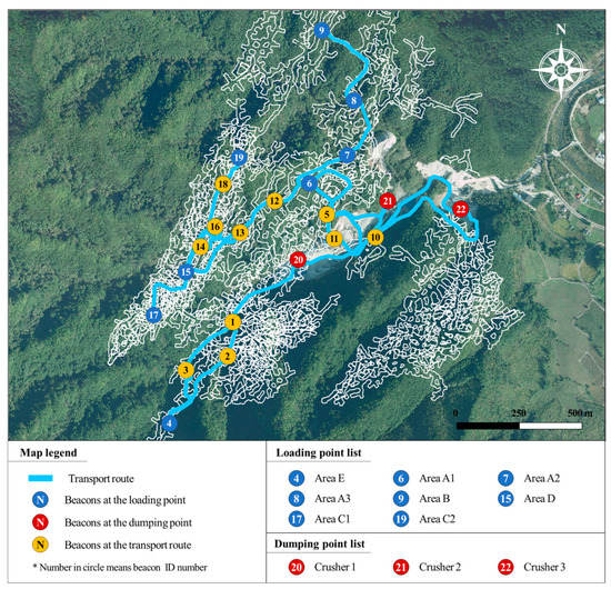
Figure 2. Bluetooth beacons installed at main locations along the haulage route.

In this study, a total of 51,732 log data were collected over a period of 15 weeks to predict the truck cycle time and ore production of the mine haulage system. Log data related to truck travel times collected using Bluetooth beacons and tablet PCs were stored in a comma-separated values (CSV) file format. When the tablet PC received the signal from the Bluetooth beacon, the ID and information set in the beacon (location division, location name), the signal reception time (date, time), and the information of the vehicle that received the signal were recorded. The location division is the information for identifying the location where the Bluetooth beacon is installed, and it is divided into loading and dumping point, entrance, haulage route, and loader.

2.2.2. Data Pre-Processing and Validation

As mentioned above, the log data record the time when the truck passes the point where the Bluetooth beacon is installed. Therefore, data pre-processing is required to calculate the truck travel time for each section. The truck travel time was calculated using the truck passage times at two points recorded sequentially, as follows: 1. The log data files recorded by the truck and the date were collected into a single data file. 2. Through division based on vehicle ID and date, a route combination (consisting of a beacon ID for the origin and the destination) was generated according to the order in which the beacon signals were received. 3. The truck travel time for each route was calculated based on the difference in the signal reception time between the two points. 4. The statistical value of the truck operation time was the output for the same route. Items of statistical value included the number of data for each route ID, average truck travel time, standard deviation, minimum and maximum travel time, and percentiles (P10, P25, P75, P90). By pre-processing 51,732 log data, 42,808 truck travel time data for 444 sections could be collected.

In this study, a time study using a stopwatch was conducted to verify the collected truck travel time data, and a production log written by truck drivers for a week was secured. The time study was performed by directly boarding a truck operating between Crusher 3 (beacon ID: 22) and Area E (beacon ID: 4) and then measuring the truck travel time with a stopwatch. The vehicle information and driving records, driving status (origin, departure time, destination, product name, etc.), maintenance details, etc., were recorded in the production log, and the truck travel time was calculated. In this study, the log data collected using a Bluetooth beacon were verified by comparing the cycle times for the section between Crusher 3 and Area E. The truck cycle time collected through the beacons and the truck cycle time calculated through the time study and production log were found to be highly similar.

3. Methods

In this study, we developed an ML–DES hybrid model that can predict the ore production of a mine haulage system by combining two techniques, machine learning and discrete event simulation. Figure 3 shows the operating principle for the ML–DES hybrid model. First, log data for the mine haulage system were collected using Bluetooth beacons and tablet PCs. The collected log data were uploaded to a cloud server and stored over a long period of time. The collected log data were pre-processed so that they could be used as input data for the ML model to predict the truck cycle time. Next, an ML model for predicting the truck cycle time was developed, and the truck cycle time was predicted for each truck and section using the pre-processed data and the data affecting the truck cycle time. Finally, the predicted truck cycle time was used as the input data for the DES model to predict ore production, and ore production by truck and loading point was predicted.

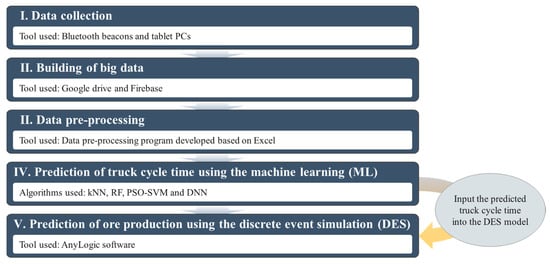
Figure 3. Operating principle of hybrid models combining machine learning (ML) and discrete event simulation (DES).

3.1. Development of Machine Learning (ML) Models for Predicting Truck Cycle Times

The ML model development for predicting the truck cycle time of the mine haulage system proceeded in the order of data collection for learning and verification, data pre-processing, ML algorithm application, ML model verification, and optimal model selection.

3.1.1. Training Data Production and Pre-Processing

In general, the truck cycle time is affected by the skill of the driver, the slope and distance of the haulage route, and environmental factors (temperature and precipitation). The higher the driving proficiency, the gentler the slope of the haulage route, and the shorter the distance, the less the truck cycle time will be. In addition, the better the road surface condition of the haulage route, the shorter the cycle time. Because the condition of the road surface in an underground mine can vary greatly depending on the amount and level of groundwater, temperature and precipitation data were considered as influencing factors. The driver’s skill is difficult to quantify. Therefore, the truck ID was used to classify the driver’s skill according to the driver. The slope and distance of the haulage route were classified using path ID. Table 2 shows the structure of the training dataset of the ML model for predicting the truck cycle time, consisting of 4 input variables and 1 label.

Table 2. Description of datasets for training machine learning models.

Dataset	Description	Data Type
Features	Path ID	Character
	Truck ID	Character
	Daily mean temperature	Float (°C)
	Precipitation	Float (mm/day)
Label	Truck cycle time	Float (min)

The truck cycle time used as a label here is composed of a series of truck travel times corresponding to travel time with an empty truck, loading time, travel time with a loaded truck, and dumping time. Therefore, when the truck cycle time is calculated by pre-processing the truck travel time data (42,808) for each section, the amount of data that can be used for the ML model is 366. Therefore, the dataset for ML model training consisted of 366 pieces of data. Categorical data included haulage routes and truck types (truck ID). Continuous data included temperature and precipitation data. The data for training the ML model consisted of the truck cycle time as collected using Bluetooth beacons, tablet PCs, and meteorological data from the KMA.

As noted above, the data types of the input variables used for ML model training consisted of categorical and continuous data. Accordingly, one-hot encoding was performed to convert categorical data into numeric data. This method prevented the problem of adding information regarding the size by converting three or more categories to an integer type; this method also created a way to solve them by creating binary characteristics for each category. The data were converted using the min–max normalization method, as shown in Equation (1).

$$x^{\prime }=\frac{x_i-\min \left(x\right)}{\max \left(x\right)-\min \left(x\right)}$$

(1)

This normalization method can prevent overfitting [41]. In addition, it is possible to increase the efficiency of ML because the parameter adjustment step and the time required for model training are reduced. The dataset for ML model training consisted of 366 data elements. The training and verification datasets were randomly divided in a 75:25 ratio, respectively, and the learned model was verified.

Before normalizing the training dataset, the statistical values for truck cycle time, precipitation, and daily mean temperature were calculated; they are presented in Table 3 and Figure 4. The mean truck cycle time (minutes) was 25.98 min, and the standard deviation was 7.43 min. During the 15 weeks, the mean and standard deviation of the daily average temperatures were −4.44 °C and 5.42 °C, respectively. The mean of the daily precipitation was 0.31 mm, and the standard deviation was 0.84 mm.

Table 3. Characteristics of datasets for training machine learning models.

Statistics	Truck Cycle Time (min)	Daily Mean Temperature (°C)	Daily Precipitation (mm/Day)
Mean	25.98	−4.44	0.31
Standard deviation	7.43	5.42	0.84
Minimum value	14.30	−14.30	0.10
Maximum value	54.50	8.80	6.90

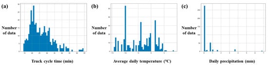
Figure 4. Characteristics of datasets to train the machine learning models: (a) truck cycle time, (b) daily mean temperature, and (c) precipitation.

3.1.2. Application of ML Algorithms

In this study, four ML algorithms were utilized to develop models for predicting the truck cycle time. The algorithms used were random forest (RF), k-nearest neighbor (kNN), support vector machine with particle swarm optimization (PSO–SVM), and DNN.

The kNN model is a type of ML model that classifies data based on the assumption that data with similar characteristics belong to the same category. Therefore, the model allocates new examples that are not classified into the classes to which the majority of the k closest neighbors belong. Misclassification of the data can be effectively reduced by increasing the number of samples in the training dataset. The accuracy of the kNN model is significantly related to the number of neighbors, k, and the distance for calculating the closest distance to the value of k [42].

The RF model is an algorithm derived from the decision tree model, which combines multiple randomly generated decision trees to form a forest-like structure. Tree-based models are popular supervised learning algorithms due to their simplicity and excellent performance. RF is an ensemble method that predicts the results by combining multiple models, and it is assumed that combining multiple models with low accuracy can achieve better performance than using one model with high accuracy. Thus, RF creates a more flexible result by summing the vertical boundaries in each tree.

The support vector machine (SVM) was initially introduced by Boser et al. [43], and it has recently been successfully applied to various problems related to pattern recognition using bioinformatics and image recognition [44]. In addition, it is a powerful and widely used algorithm that can be used for both linear and nonlinear regression and classification. SVM is basically a model that linearly classifies data like linear logistic regression and classifies data in three stages. Assuming that there are two-dimensional data composed of two classes, there can be an infinite number of straight lines separating these classes, but only one straight line can be selected using the condition for selecting the decision boundary of SVM. The selection condition is to select a hyperplane that maximizes the distance between the closest data points of each class. The closest points between each class are selected, and when the distance between margins represented by two parallel straight lines containing these points is maximized, two straight lines containing these points are selected. The points used to select the two straight lines are called support vectors, and when these two straight lines are determined, the central straight line located at the same distance from the two straight lines becomes the decision boundary [45].

The PSO–SVM model combines particle swarm optimization (PSO) to optimize the SVM parameters. The PSO is an optimization technique that simulates the diversity of swarms based on the behavior of particles and social animals, such as flocks of flying birds. It was developed in 1995 by Kennedy and Eberhart [46]. The PSO is a computational algorithm inspired by swarm intelligence. Swarm intelligence arises from populations or homogeneous cooperation in a particle environment and assumes that each particle has a specific size with an arbitrary starting position. In PSO–SVM, the particles are denoted as C and $\mathsf{\gamma }$, and they are the hyperparameters of SVM. Speed ($v_i$) was calculated using Equation (2), and position ($x_i$) was calculated using the calculated speed (Equation (3)). In this manner, each particle moves around the area and shares the optimal hyperparameter position to find a hyperparameter that converges [47]. In Equations (2) and (3), $j$ is the particle index, $i$ is the iteration, $v_j$ is the particle speed, $x_j$ is the particle position, $P_{best}$ is the best value of the particle, $G_{best}$ is the best iteration value, $C_1$ is the learning rate, and $r_1$ is a random number.

$$v_j\left(i+1\right)=v_j\left(i\right)+c_1{r}_1(P_{best}-x_j\left(i\right))+c_1{r}_1(G_{best}-x_j\left(i\right))$$

(2)

$$x_j\left(i+1\right)=x_j\left(i\right)+v_j\left(i+1\right)$$

(3)

The DNN model is an algorithm based on the use of ANNs to process information in a form similar to that used in the human brain by receiving a motif from the structure of a human neural network. Deep learning has the advantage of not having to inform users of the importance of data attributes. The DNN model has a layered structure consisting of an input layer, multiple hidden layers, and an output layer. The data are input, and by stacking neural layers, they undergo several stages of feature extraction to automatically extract high-level abstract knowledge. Data are transmitted through the repetition of information transfers and operations between nodes corresponding to human neurons, and through the transfer of computational results. The prediction accuracy of the DNN-based model is determined by the number of hidden layers and nodes. Accordingly, the optimal model must be determined by adjusting this number.

Various parameters exist depending on the ML algorithm, and the performance of the ML model depends on these parameters. In this study, the kNN, RF, and DNN models had their parameters optimized using grid search (GS) through 5-fold cross-validation. The SVM model’s parameters were optimized using PSO. The parameter types and tunings for each ML model used in this study are listed in Table 4.

Table 4. Values for parameter tuning by grid search.

Model	kNN	RF	PSO–SVR	DNN
Parameter	n_neighbors	n_estimators ccp_alpha/ min_impurity_decrease/ min_samples_leaf/ min_samples_split/ min_weight_fraction_leaf	C/$\mathsf{\gamma }$	Hidden layer node
Min	1	100/0/0/1/1/0.1	10/0.1	2/20
Max	100	100/10/10/10/10/1	100/1	10/100
Step	(+) 1	(+) 0/1/1/1/1/0.1	-	(+) 1/10

For the kNN model, the accuracy depends on the value of k (n_neighbors), which represents the number of neighbors considered. The accuracy was predicted by incrementing k from 1 to 100. In the case of the RF model, various parameters, such as n_estimators, ccp_alpha, min_impurity_decrease, min_samples_leaf, min_samples_split, and min_weight_fraction_leaf, were tuned to maximize accuracy. For each parameter, a specific range was set, and the accuracy was predicted accordingly. n_estimators is a parameter that indicates the number of trees to be created. ccp_alpha is a parameter indicating the complexity used for least-cost-complexity pruning. min_impurity_decrease indicates the minimum amount of impurity reduction obtained through division. min_samples_leaf is the minimum number of sample data points required to become a leaf node, and min_samples_split is the minimum number of sample data points required to split a node. min_weight_fraction_leaf is similar to min_samples_leaf, but it is a ratio of the total number of weighted samples.

The accuracy of the PSO–SVR model depends largely on the parameters C and $\gamma$. C denotes a parameter that specifies the extent to which the SVR model can tolerate an error. $\gamma$ determines how flexibly the decision boundary is drawn. Parameters C (10–100) and $\gamma$ (0.1–1) were optimized using a particle swarm optimization.

Because the accuracy of the DNN model varies depending on the hidden layer and the node, the hidden layer was set from 2 to 10 and the node was set from 20 to 100, and then they were increased by 1 and 10, respectively, to increase the accuracy of the model.

3.1.3. ML Model Verification and Optimal Model Selection

The performance of the ML model was verified using the mean absolute error (MAE), mean square error (MSE), root mean square error (RMSE), and coefficient of determination (R²), which are the performance indicators representing the performance of the regression model in this study. MAE refers to the value obtained by averaging the absolute value of the error (the difference between the actual and predicted values, Equation (4)). The MSE represents the average of the squares of the errors (Equation (5)). RMSE refers to the square root of the MSE and allows for the examination of the magnitude of the error (Equation (6)). R² represents the extent to which the regression equation can explain the original data (Equation (7)). The equations for each performance indicator are as follows, where $h\left(x^{\left(i\right)}\right)$ is the predicted value from the model of the i-th data and $y^i$ is the label of the i-th data. The sum of squares for the residual is the sum of the results obtained by subtracting the average of the observed values from the estimated value. The total sum of squares indicates the sum of the results obtained by subtracting the average of the observed values from the observed value.

$$MAE\left(X,h\right)=\frac{1}{n}{\sum }_{i=1}^n\left|h(x^{\left(i\right)}-y^{\left(i\right)}\right|$$

(4)

$$MSE\left(X,h\right)=\frac{1}{n}{\sum }_{i=1}^n{\left(h\right(x^{\left(i\right)}-y^{\left(i\right)})}^2$$

(5)

$$RMSE\left(X,h\right)=\sqrt{\frac{1}{n}{\sum }_{i=1}^n\left|h(x^{\left(i\right)}-y^{\left(i\right)})\right|}$$

(6)

$$R^2=1-\frac{SSE}{SST}$$

(7)

3.2. Development of a Production Prediction ML–Discrete Event Simulation (DES) Model

3.2.1. Design of ML–DES Model

A DES model was designed to predict ore production in the study area by using the truck cycle time predicted by the ML model as input data. Figure 5 shows a schematic diagram of the input data used to predict the ore production and output data after simulation using the DES model to simulate the mine haulage system. The input data of the simulation model were divided into simulation factors related to the operating conditions and time factors related to the time required for the unit tasks. The simulation parameters related to the operating conditions included the operating time (simulation time), truck ID, truck capacity, and loading point, and the time parameters included the travel time, loading time, and dumping time. The output data of the simulation model included the total operating time, number of loading and haulage, amount of loaded ore, and time of haulage for one cycle.

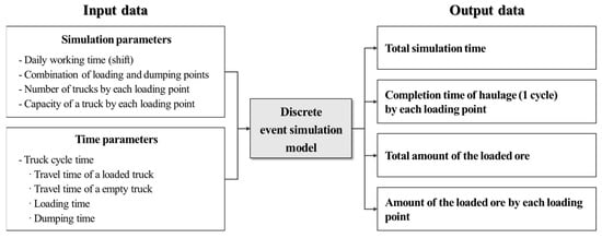
Figure 5. Input and output parameters for simulating the truck haulage system.

The simulation parameters can be determined through interviews with the field staff and an analysis of the vehicle operation log. For the parameters related to time, such as truck travel time, the cycle time for each truck allocation scenario, as predicted using the ML model, was used.

3.2.2. Development of Simulation Algorithm

Figure 6 shows the simulation algorithm for the mine haulage system designed according to the research area and truck cycle time (TCT) theory. The TCT theory was proposed by Suboleski [48], and it can be explained using the following equation:

$$TCT=STL+LT+TL+STD+DT+TE+AD$$

(8)

where TCT means truck cycle time, STL is the spotting time in the loader, LT is the loading time, TL is the travel time of the loaded truck, STD is the spotting time in the dumping point, DT is the dumping time, TE is the travel time of the empty truck, and AD denotes the average delay time. This is the delay time that can be caused by the truck waiting for work at the loading or dumping point. The truck dispatched into the system was designed to move to a designated loading point, transport the ores to the crusher, and continue to perform the operation for a simulation time set in advance by the user. In this study, a simulation model reflecting the designed simulation algorithm was developed and implemented using the AnyLogic software, as shown in Figure 7. In addition, the layout of the simulation model was designed considering loading and dumping points and haulage routes, as shown in Figure 2. The simulation model in Figure 7 shows the model for one truck allocated to one specific loading point and can be expanded by considering the types and numbers of trucks and the number of loading points. Table 5 presents the functions of each block in the simulation model.

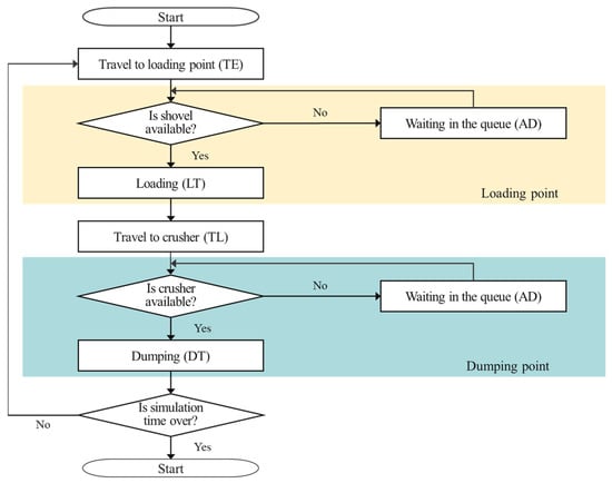
Figure 6. Algorithm for simulation of truck haulage system.

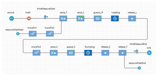
Figure 7. Implementation of a truck haulage system simulation using AnyLogic software.

Table 5. Functions of each block in the discrete event simulation model.

Blocks	Function
source	Start of the truck haulage system Creation of ore to be loaded and transported (at the loading point)
sink	Termination of truck haulage system Removal of loaded and transported ore (at the dumping point)
hold	Control the start and termination of the simulation
TimeMeasureStart	Measure the time it takes to load and haul ore once
timeMeasureEnd
resourceTaskStart	Creation of trucks to carry out the loading and hauling of ore
resourceTaskEnd	Removal of trucks to carry out the loading and hauling of ore
moveTo1	Moving to the loading point of the empty truck
moveTo2	Moving to the loading point of the empty truck
moveTo3	Moving to the dumping point of the loaded truck
seize_T	Designation of truck to carry out ore loading and hauling operations
seize_L	Designation of loader to perform loading operation
seize_C	Designation of crusher to perform dumping operation
release_T	Deselection of truck that has completed loading and hauling operations
release_L	Deselection of loader that has completed loading operation
release_C	Deselection of crusher that has completed dumping operation
Loading	Loading operation
Dumping	Dumping operation
queue_C	Queues created at dumping points
queue_LP	Queues created at loading points

3.2.3. Verification of Simulation Algorithm

The simulation algorithm was verified by comparing the simulation results with data from the analysis of the vehicle operation log for a week. The simulation was performed using the TCT predicted by the ML model for the input data. To this end, the section (crushing field to loading field), time, and production volume were analyzed for each truck during the corresponding period using the vehicle operation log. Additional verification was performed by comparing the times the ores were loaded and dumped with the time output from the DES model on the working day when the vehicle operation log was written.

4. Results

4.1. Results of Development of Cycle Time Prediction ML Model

4.1.1. Results of ML Model Training

Four ML models (kNN, RF, PSO–SVM, and DNN) were used to predict the TCT. For each model, the parameters related to the learning accuracy listed in Table 4 were optimized, and a predictive model with the best performance was designed. The prediction accuracy of the kNN model depends on parameter k. Figure 8a shows the accuracy of the model by increasing k by 1 from 1 to 100. The prediction accuracy of the kNN model was highest when k = 53. Based on the training dataset, the MAE shows the lowest error of 3.74 min. The accuracy of the RF model is related to six hyperparameters. Figure 8b illustrates the learning accuracy of the RF model, which varies owing to changes in the parameter values. The RF has the lowest error of 3.83 (min) when n_estimators is 100, ccp_alpha is 2, min_impurity_decrease is 2, min_samples_leaf is 6, min_samples_split is 5, and min_weight_fraction_leaf is 0. The learning accuracy of the PSO–SVM model is determined by the parameters C and $\gamma$, and Figure 8c shows the learning accuracy of the model according to changes in the parameters C and $\gamma$. The PSO–SVM model showed the best performance with an MAE of 3.45 (min) when C was set to approximately 30.21 and $\gamma$ to approximately 0.61. The learning accuracy of the DNN model varied according to the number of hidden layers and nodes. Figure 8d shows the learning accuracy of the model according to changes in the parameters. The DNN model showed the smallest error (MAE = 3.97 (min)) when the number of hidden layers was 9 and the number of nodes was 20.

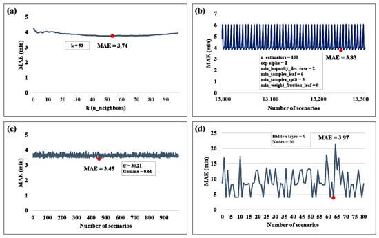
Figure 8. Learning accuracy of machine learning models by hyperparameter tuning: (a) kNN; (b) RF; (c) PSO–SVR; (d) DNN.

4.1.2. Results of Performance Evaluation of Cycle Time Prediction Model

After applying the parameter with the highest learning accuracy to each model, the performance was evaluated based on verification data (25% of the total data). Figure 9 shows the actual measured TCT and the predicted values from the model. In the graph, the horizontal axis represents the actual TCT and the vertical axis represents the value predicted by the ML model. All four models were found to be biased towards the maximum and minimum values of TCT predictions.

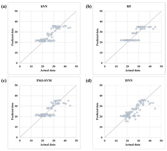
Figure 9. Actual measured truck cycle time and predicted values of the machine learning model: (a) kNN; (b) RF; (c) PSO–SVR; (d) DNN.

The performance of the ML model was evaluated using MAE, MSE, RMSE, and R², which are performance indicators mainly used in regression models. Table 6 shows the performance index of each model. The performance indicators for the kNN model are as follows: MAE of 2.89 (min), MSE of 13.65 (min²), RMSE of 3.69 (min), and R² of 0.69 (Figure 9a). The RF model was confirmed to be biased towards the maximum and minimum values of the cycle time prediction (Figure 9b). In addition, the values of the performance indicators were as follows: MAE, 2.88 (min); MSE, 15.40 (min²); RMSE, 3.92 (min); and R², 0.65. The results from the PSO–SVR model are shown in Figure 9c. Owing to the difference between the predicted values and the actual data, the MAE is 2.79 (min), MSE is 14.29 (min²), RMSE is 3.78 (min), and R² is 0.68. The verification results of the DNN model are presented in Figure 9d. The MAE is 2.95 (min), MSE is 16.14 (min²), RMSE is 4.02 (min), and R² is 0.64.

Table 6. Indicators for performance assessment of the machine learning models.

Indicator	kNN	RF	PSO–SVR	DNN
MAE (min)	2.89	2.88	2.79	2.95
MSE (min2)	13.65	15.40	14.29	16.14
RMSE (min)	3.69	3.92	3.78	4.02
R2	0.69	0.65	0.68	0.64

In this study, the performance ranking of ML models for predicting TCT based on MAE among four performance indicators was determined. MSE is sensitive to outliers because it is calculated by squaring the difference between the predicted value and the actual value. That is, when the error between the predicted value and the actual value is between 0 and 1, the error is reflected in the MSE as smaller than the original error, and when the error is larger than 1, the error is reflected as larger than the original error. Because RMSE is calculated by taking the root of MSE, it can compensate for the disadvantages of MSE, but each error has a different weight. On the other hand, in the case of MAE, compared to MSE and RMSE, the influence of outliers is relatively small, and equal weights are given to all errors. Therefore, when the performance of the ML model is determined based on the MAE, the PSO–SVM model appears to have the best performance. The PSO–SVM model showed the lowest error with an MAE of 2.79 (min), followed by RF, kNN, and DNN. It should be noted that the PSO–SVM model shows the best performance as a model for predicting TCT.

4.2. Results of the Production Prediction ML–DES Model

4.2.1. Settings of Simulation Scenario and Parameters

Using AnyLogic software, the ML–DES model was developed to predict ore production, and verification was performed to determine whether the mine haulage system in the research area was properly simulated. The simulation model was verified by comparing the analysis results from the vehicle operation log, as secured in advance, with the results from the simulation by applying the operating conditions from the period in which the log was written. By analyzing the vehicle operation log, it was found that the trucks used in the haulage system generally perform work for 8 h a day (08:00–17:00), excluding lunch time (1 h). However, it was found that the haulage route frequently changed because of daily production plans and unexpected variables potentially occurring at the site (crusher failure, temporary closure of the mine, etc.). As a result of the vehicle operation log analysis, ore was produced using four routes, as shown in Table 7, during the period. Table 8 presents the simulation scenario and input data, as determined through the vehicle operation log analysis.

Table 7. Routes for ore production derived from analysis of vehicle operation log analysis.

Route ID	Loading Point	Dumping Point	Beacon IDs
A	Area A	Crusher 3	4 ↔ 2 ↔ 1 ↔ 20
B	Area B	Crusher 3	9 ↔ 8 ↔ 7 ↔ 6 ↔ 5 ↔ 20
C	Area C1	Crusher 1	17 ↔ 16 ↔ 14 ↔ 13 ↔ 12 ↔ 6 ↔ 11 ↔ 10 ↔ 22
D	Area C2	Crusher 1	19 ↔ 18 ↔ 16 ↔ 14 ↔ 13 ↔ 12 ↔ 6 ↔ 11 ↔ 10 ↔ 22

Table 8. Simulation scenario and input data determined through vehicle operation log analysis.

Date	Truck ID	Truck Type (tons)	Route ID	Operating Time (Simulation Time, hh:mm)
23 November 2020	1	37.5	A	08:00~12:00
	6	23.0	C	10:00~12:00, 13:00~14:30
	4	23.0	C	09:00~12:00, 13:00~14:30
	7	23.0	C	10:00~12:00, 13:00~14:30
24 November 2020	3	23.0	B	08:00~12:00, 13:00~17:00
25 November 2020	1	37.5	A	08:00~12:00, 13:00~14:30
	2	37.5	A	08:00~12:00, 13:00~14:30
	3	23.0	B	08:00~12:00, 13:00~17:00
26 November 2020	1	37.5	A	14:00~16:30
	2	37.5	A	14:00~16:00
	3	23.0	B	08:00~12:00, 13:00~16:30
	6	23.0	D	08:00~12:00, 13:00~16:30
	5	23.0	D	08:00~12:00, 13:00~16:30
	4	23.0	D	08:00~11:00
	7	23.0	D	08:00~10:30
27 November 2020	1	37.5	A	08:00~12:00, 13:00~15:00
	2	37.5	A	08:00~12:00, 13:00~15:00
	6	23.0	D	13:00~17:00
	4	23.0	D	13:00~17:00
	7	23.0	D	13:00~17:00
28 November 2020	3	23.0	B	08:00~12:00, 13:00~17:00
	5	23.0	C	10:30~12:00, 13:00~15:30
	4	23.0	C	10:30~12:00, 13:00~15:30
	7	23.0	C	10:30~12:00, 13:00~15:30
	6	23.0	D	08:00~10:30
	5	23.0	D	08:00~10:30
	4	23.0	D	08:00~10:30
	7	23.0	D	08:00~10:30

The truck travel time for each section, as input to the DES model, was calculated using the TCT prediction ML model. The truck travel time input to the simulation model has the form of mean ± standard deviation. Table 9 summarizes the time data by truck and section. It is assumed that the loading and dumping times of the ore vary depending on the type of truck and that they have the same values in all sections.

Table 9. Truck travel time by truck/section calculated using the truck cycle time prediction model.

Truck ID	Route ID	Travel Time with Empty Truck (Mean ± SD)	Loading Time (Mean ± SD)	Travel Time with Loaded Truck (Mean ± SD)	Dumping Time (Mean ± SD)
1	A	8.83 ± 1.77	3.73 ± 0.75	8.23 ± 1.65	0.62 ± 0.12
	C	13.13 ± 2.63	3.73 ± 0.75	12.24 ± 2.45	0.62 ± 0.12
2	A	9.14 ± 1.83	3.73 ± 0.75	8.52 ± 1.7	0.62 ± 0.12
	B	12.22 ± 2.44	3.73 ± 0.75	11.39 ± 2.28	0.62 ± 0.12
	C	16.36 ± 3.27	3.73 ± 0.75	15.26 ± 3.05	0.62 ± 0.12
3	B	12.38 ± 2.48	4.05 ± 0.81	9.67 ± 1.93	0.88 ± 0.18
4	C	16.57 ± 3.31	4.05 ± 0.81	12.94 ± 2.59	0.88 ± 0.18
	D	16.07 ± 3.21	4.05 ± 0.81	12.55 ± 2.51	0.88 ± 0.18
5	C	18.28 ± 3.66	4.05 ± 0.81	14.28 ± 2.86	0.88 ± 0.18
	D	13.24 ± 2.65	4.05 ± 0.81	10.34 ± 2.07	0.88 ± 0.18
6	C	16.79 ± 3.36	4.05 ± 0.81	13.12 ± 2.62	0.88 ± 0.18
	D	14.47 ± 2.89	4.05 ± 0.81	11.3 ± 2.26	0.88 ± 0.18
7	C	17.04 ± 3.41	4.05 ± 0.81	13.31 ± 2.66	0.88 ± 0.18
	D	14.93 ± 2.99	4.05 ± 0.81	11.66 ± 2.33	0.88 ± 0.18

4.2.2. Results and Verification of Simulations

In this study, the ML–DES model for ore production prediction was verified by comparing the production by truck/section, as recorded in the vehicle operation log, with the ore production calculated through the simulation model. The simulation was performed by inputting the previously determined simulation scenario, input data, and truck operation time data. Because the vehicle operation log written in the field is based on the loading time, the simulation model was also set to count the amount of transportation of the ore at the time of loading the ore. Table 10 and Figure 10 show the ore production (tons) and the number of transports by dividing the vehicle operation log and simulation prediction results by truck/section. In the case of morning operations, it should be noted that the simulation model predictions are generally similar to those from the vehicle operation log. However, in the case of afternoon operations, there is a slight difference in the prediction results; however, the analysis and prediction results are correlated with each other.

Table 10. Comparison of production between vehicle operation log and discrete event simulation model.

Date	Truck ID	Route ID	Vehicle Operation Log		Discrete Event Simulation
			Amount of Loaded Ores (tons)		Amount of Loaded Ores (tons)
			AM (08:00~12:00)	PM (13:00~17:00)	AM (08:00~12:00)	PM (13:00~17:00)
23 November 2020	1	A	412.5	-	412.5	-
	6	C	112.5	112.5	150.0	112.5
	4	C	187.5	112.5	187.5	112.5
	7	C	112.5	112.5	150.0	75.0
24 November 2020	3	B	300.0	300.0	375.0	375.0
25 November 2020	1	A	337.5	75.0	450.0	150.0
	2	A	412.5	37.5	412.5	150.0
	3	B	300.0	337.5	337.5	337.5
26 November 2020	1	A	-	262.5	-	300.0
	2	A	-	187.5	-	187.5
	3	B	300.0	225.0	412.5	300.0
	6	D	262.5	225.0	262.5	262.5
	5	D	262.5	187.5	300.0	300.0
	4	D	225.0	-	187.5	-
	7	D	150.0	-	187.5	-
27 November 2020	1	A	375.0	150.0	412.5	187.5
	2	A	375.0	187.5	412.5	187.5
	6	D	-	337.5	-	262.5
	4	D	-	337.5	-	262.5
	7	D	-	337.5	-	300.0
28 November 2020	3	B	300.0	300.0	412.5	337.5
	5	C	75.0	187.5	112.5	187.5
	4	C	75.0	187.5	112.5	187.5
	7	C	75.0	187.5	112.5	150.0
	6	D	187.5	-	187.5	-
	5	D	187.5	-	187.5	-
	4	D	150.0	-	150.0	-
	7	D	187.5	-	187.5	-

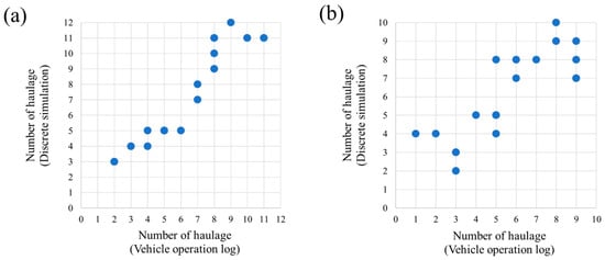
Figure 10. Comparison of production between vehicle operation log and discrete event simulation model: (a) morning operation; (b) afternoon operation.

In this study, additional verification of the DES model was performed by organizing the loading time of the ore using the vehicle operation log of 26 November 2020 and comparing it with the loading time simulated in the model. Table 11 shows the loading times calculated in the vehicle operation log and the simulation model divided by section, truck, and time zone. As a result, discrepancies occur between the vehicle operation log and the simulation model for some trucks and sections, but the loading times and transportation frequency are generally similar. The trucks and sections where the simulation model does not predict accurately may not have predicted the cycle time with high accuracy owing to a relative lack of training data in the TCT prediction ML model. In addition, as the DES model has a limitation in that it cannot consider variables or situations occurring abnormally during actual haulage operations, trucks and sections with low prediction accuracy can occur. Therefore, there should be sufficient data accumulation for training the ML model to enhance the DES model. Improvement is necessary for the simulation model to better reflect reality.

Table 11. Comparing the loading time between the vehicle operation log and the predicted result of the machine learning–discrete event simulation model.

Time	Route A				Route B		Route D
	Truck 1		Truck 2		Truck 3		Truck 4		Truck 5		Truck 6		Truck 7
	Actual Log	DES	Actual Log	DES	Actual Log	DES	Actual Log	DES	Actual Log	DES	Actual Log	DES	Actual Log	DES
8:00					08:10 08:40	08:11 08:35 08:58	08:19 08:51	08:27	08:34	08:16 08:21	08:25 08:58	08:19 08:45	08:29	08:24 08:54
9:00					09:10 09:38	09:17 09:41	09:21 09:51	09:05 09:48	09:06 09:36	09:09 09:34	09:27 09:56	09:21 09:54	09:02 09:31	09:25 09:51
10:00					10:06 10:33	10:09 10:33 10;58	10:20 10:48	10:19 10:53	10:05 10:35	10:03 10:31	10:25 10:52	10:27	10:01	10:24
11:00					11:00 11:27	11:22 11:47			11:02 11:35	11:06 11:43	11:26	11:03 11:39
12:00	Lunch time
13:00					13:17 13:43	13:15 13:35			13:23	13:18 13:24	13:13 13:44	13:22 13:29
14:00	14:00 14:25 14:51	14:07 14:27 14:46	14:10 14:37 14:57	14:22 14:41	14:12 14:42	14:00 14:27 14:49			14:05 14:53	14:14 14:37	14:38	14:18 14:45
15:00	15:08 15:28 15:46	15:04 15:26 15:46	15:17 15:38	15:07 15:30 15:52	15:14 15:56	15:15 15:41			15:21 15:50	15:04 15:30 15:55	15:03 15:29	15:19 15:50
16:00	16:05	16:04 16:26				16:15				16:21	16:02	16:23
Number of haulage	7	8	5	5	14	18	6	5	12	16	13	14	4	5

5. Discussion

The truck cycle time can be predicted using data related to the truck travel time as recorded using tablet PCs and Bluetooth beacons, and the predicted results can be entered into the DES model to predict ore production by truck and section and to determine the optimal number of trucks dispatched to the workplace. Based on the haulage system in the study area, daily operating conditions were assumed, then the simulation was performed, and an optimal truck dispatch plan was derived. To this end, the following assumptions were made: (1) The haulage operation was performed for 8 h (540 min) per day. (2) Six trucks (two 37.5-ton trucks (truck IDs 1 and 2) and four 23-ton trucks (truck IDs 4–7) were dispatched to three loading points (loading points A, C, and D). (3) Each loading point produced limestone of different grades. (4) To achieve the target grade, at least 600, 800, and 700 metric tons of limestone were produced at each loading point. Based on these four assumptions, 39 truck–dispatch combinations were determined. The truck travel times for each truck and section input to the simulation model were calculated using the TCT prediction ML model and converted to mean ± standard deviation format.

The simulation was conducted by entering the daily operating conditions and truck travel time data; 13 of the 39 truck dispatch combinations met the minimum production target for each loading point (Table 12). Loading point A (route A) can achieve its target ore production with one 37.5-ton truck. Loading point C (route C) can achieve the target production only when one 37.5-ton truck and one or two 23-ton trucks are dispatched. Loading point D (route D) should be dispatched with two or three 23-ton trucks. Based on the total ore production, scenario ID 23 produced the most limestone during the working hours per day (2995 metric tons). In addition, even in the case of the time required to achieve the target production per day, scenario ID 23 required the least time (386 min) to meet the target production (Table 13). Looking at the ore production by loading point when the target production was achieved, 675 metric tons of limestone were produced at loading point A, 801 metric tons at C, and 897 metric tons at D.

Table 12. Combinations of trucks that can meet the daily target production.

Scenario ID	Truck 1	Truck 2	Truck 4	Truck 5	Truck 6	Truck 7
	37.5 tons	37.5 tons	23 tons	23 tons	23 tons	23 tons
19	A	C	C	D	D	C
20	A	C	D	D	C	C
23	A	C	C	D	D	D
24	A	C	D	C	D	D
25	A	C	D	D	C	D
26	A	C	D	D	D	C
31	C	A	C	C	D	D
32	C	A	C	D	D	C
33	C	A	D	D	C	C
36	C	A	C	D	D	D
37	C	A	D	C	D	D
38	C	A	D	D	C	D
39	C	A	D	D	D	C

Table 13. Simulation results for the truck–dispatch combination for achieving the daily target production.

Scenario ID	Ore Production (tons)										Time Required to Achieve Target Production (min)
	By Truck						By Route (Loading Points)			Total
	1	2	4	5	6	7	A	C	D
19	862.5	637.5	345.0	391.0	345.0	299.0	862.5	1281.5	736.0	2880.0	466
20	900.0	600.0	299.0	414.0	368.0	299.0	900.0	1267.0	713.0	2880.0	480
23	862.5	637.5	368.0	414.0	345.0	368.0	862.5	1005.5	1127.0	2995.0	386
24	825.0	637.5	299.0	345.0	345.0	368.0	825.0	982.5	1012.0	2819.5	399
25	862.5	600.0	299.0	414.0	345.0	345.0	862.5	945.0	1058.0	2865.5	411
26	862.5	600.0	299.0	414.0	345.0	299.0	862.5	899.0	1058.0	2819.5	405
31	600.0	825.0	345.0	345.0	368.0	345.0	825.0	1290.0	713.0	2828.0	471
32	600.0	862.5	345.0	391.0	322.0	299.0	862.5	1244.0	713.0	2819.5	464
33	600.0	825.0	299.0	414.0	368.0	299.0	825	1267.0	713.0	2805.0	474
36	637.5	862.5	345.0	414.0	322.0	368.0	862.5	982.5	1104	2949.0	390
37	600.0	825.0	276.0	368.0	345.0	368.0	825.0	968.0	989.0	2782.0	403
38	637.5	825.0	299.0	391.0	368.0	391.0	825.0	1005.5	1081.0	2911.5	393
39	637.5	825.0	299.0	414.0	345.0	299.0	825.0	936.5	1058.0	2819.5	422

6. Conclusions

In this study, a hybrid model combining ML and DES techniques is proposed to predict the ore production of a mine haulage system. The hybrid model was designed to predict ore production by linking the TCT predicted by the ML model with the DES model. For this purpose, a limestone mine in Korea was selected as the research area, and truck travel times of the underground mine were recorded for a certain period using tablet PCs and Bluetooth beacons. Four models of kNN, RF, PSO–SVM, and DNN were developed for TCT prediction, and performance evaluation of the models was performed. As a result of evaluating the performance of the ML model using a verification dataset, the PSO–SVM model showed the best performance. The MAE of PSO–SVM was 2.79 (min), representing the lowest error among the four models, and the other values were 14.29 (min²) for the MSE, 3.78 (min) for the RMSE, and 0.68 for R². The ML–DES model for production prediction was developed using the AnyLogic software. After predicting the truck cycle time by truck/section using the PSO–SVM model and inputting it into the simulation model, verification was performed on whether the simulation model properly simulated the truck haulage system. The model was verified by comparing the analysis results from the vehicle operation log with simulation results. In the case of the morning work, the simulation model predictions were similar to the analysis results from the vehicle operation log. However, in the case of the afternoon work, there was a slight difference in the prediction results; nevertheless, the analysis and prediction results were found to be correlated with each other.

The ML–DES model for production prediction developed in this study could predict TCTs using the log data of truck operation times. In addition, by entering the predicted results into the simulation model, it was proven that production by truck and section could be predicted and that the optimal truck dispatch combination for each loading point could be determined. The proposed model solved the problems concerning the degradation of prediction accuracy and verification of the prediction results that may occur in existing DES and single ML techniques. Accordingly, they can be used at any point during the development of underground mines. In other words, even if the TCT changes owing to the continued development and depth of the ore body (e.g., if it deepens) and/or if the haulage distance from the crusher to the loading point increases, production can be predicted using the model. In addition, the developed model can be utilized in decision-making processes related to the establishment of an arrangement plan for existing equipment according to the daily production plan and the selection and input of new equipment. Furthermore, the hybrid model combining ML and DES is expected to be fully utilized not only in the mining field but also in other industries.

References

- Alarie, S.; Gamache, M. Overview of Solution Strategies Used in Truck Dispatching Systems for Open Pit Mines. Int. J. Surf. Min. Reclam. Environ. 2002, 16, 59–76. [Google Scholar] [CrossRef]
- Osanloo, M.; Paricheh, M. In-pit crushing and conveying technology in open-pit mining operations: A literature review and research agenda. Int. J. Min. Reclam. Environ. 2020, 34, 430–457. [Google Scholar] [CrossRef]
- Bao, H.; Knights, P.; Kizil, M.; Nehring, M. Electrification Alternatives for Open Pit Mine Haulage. Mining 2023, 3, 1–25. [Google Scholar] [CrossRef]
- Hartman, H.L.; Mutmansky, J.M. Unit operations of mining. In Introductory Mining Engineering, 2nd ed.; Wiley: New York, NY, USA, 2002; pp. 119–152. [Google Scholar]
- Ercelebi, S.G.; Bascetin, A. Optimization of shovel-truck system for surface mining. J. S. Afr. Inst. Min. Metall. 2009, 109, 433–439. [Google Scholar]
- Choi, Y.; Nieto, A. Optimal haulage routing of off-road dump trucks in construction and mining sites using Google Earth and a modified least-cost path algorithm. Autom. Constr. 2011, 20, 982–997. [Google Scholar] [CrossRef]
- Choi, Y.; Nieto, A. Software for simulating open-pit truck/shovel haulage systems using Google Earth and GPSS/H. J. Korean Soc. Miner. Energy Resour. Eng. 2011, 48, 734–743. [Google Scholar]
- Matamoros, M.E.V.; Dimitrakopoulos, R. Stochastic short-term mine production schedule accounting for fleet allocation, operational considerations and blending restrictions. Eur. J. Oper. Res. 2016, 255, 911–921. [Google Scholar] [CrossRef]
- Jung, D.; Baek, J.; Choi, Y. Stochastic Predictions of Ore Production in an Underground Limestone Mine Using Different Probability Density Functions: A Comparative Study Using Big Data from ICT System. Appl. Sci. 2021, 11, 4301. [Google Scholar] [CrossRef]
- Rist, K. The solution of a transportation problem by use of a Monte Carlo technique, mining world. In Proceedings of the 1st APCOM, Tucson, AZ, USA, November 1961. [Google Scholar]
- Douglas, J. Prediction Shovel-Truck Production, A Reconciliation of Computer and Conventional Estimates; Stanford University: Stanford, CA, USA, 1964. [Google Scholar]
- Doe, D.C.; Griffin, W.F. Experimental design and mining system simulation. Continuous surface mining. In Proceedings of the 1st International Symposium on Continuous Surface Mining, Edmonton, AB, Canada, 29 September–1 October 1986; Golosinski, T.S., Boehm, F.G., Eds.; Trans Tech Publications Inc.: Zürich, Switzerland, 1986; pp. 317–324. [Google Scholar]
- Sturgul, J.R.; Harrison, J. Simulation models for surface mines. Int. J. Min. Reclam. Environ. 1987, 1, 187–189. [Google Scholar] [CrossRef]
- Harrison, J.; Sturgul, J.R. GPSS computer simulation of equipment requirements for the iron duke mine. In Proceedings of the Australasian Institute of Mining and Metallurgy, Second Large Open Pit Mining Conference, Latrobe Valley Vic, Gippsland, VIC, Australia, April 1988; pp. 133–136. [Google Scholar]
- Basu, A.J.; Baafi, E.Y. Discrete event simulation of mining systems: Current practice in Australia. Int. J. Surf. Min. Reclam. Environ. 1999, 13, 79–84. [Google Scholar] [CrossRef]
- Vagenas, N. Applications of discrete-event simulation in Canadian mining operations in the nineties. Int. J. Surf. Min. Reclam. Environ. 1999, 13, 77–78. [Google Scholar] [CrossRef]
- Awuah-Offei, K.; Temeng, V.A.; Al-Hassan, S. Predicting equipment requirements using SIMAN simulation—A case study. Min. Technol. 2003, 112, 180–184. [Google Scholar] [CrossRef]
- Burt, C.N.; Caccetta, L. Match factor for heterogeneous truck and loader fleets. Int. J. Surf. Min. Reclam. Environ. 2007, 21, 262–270. [Google Scholar] [CrossRef]
- Smith, S.D.; Wood, G.S.; Gould, M. A new earthworks estimating methodology. Constr. Manag. Econ. 2000, 18, 219–228. [Google Scholar] [CrossRef]
- Choi, Y. New software for simulating truck-shovel operation in open pit mines. J. Korean Soc. Miner. Energy Resour. Eng. 2011, 48, 448–459. [Google Scholar]
- Dindarloo, S.R.; Osanloo, M.; Frimpong, S. A stochastic simulation framework for truck and shovel selection and sizing in open pit mines. J. S. Afr. Inst. Min. Metall. 2015, 115, 209–219. [Google Scholar] [CrossRef]
- Krause, A.; Musingwini, C. Modelling open pit shovel-truck systems using the machine repair model. J. S. Afr. Inst. Min. Metall. 2007, 107, 469–476. [Google Scholar]
- Lee, C.; Choi, Y. Integration of simulation and animation for truck-loader haulage systems in an underground mine using GPSS/H and PROOF5. J. Korean Soc. Miner. Energy Resour. Eng. 2018, 55, 185–193. [Google Scholar] [CrossRef]
- Jung, D.; Baek, J.; Choi, Y. Simulation and Real-time Visualization of Truck-Loader Haulage Systems in an Open Pit Mine using AnyLogic. J. Korean Soc. Miner. Energy Resour. Eng. 2020, 57, 45–57. [Google Scholar] [CrossRef]
- Torkamani, E.; Askari-nasab, H. Verifying Short-Term Production Schedules using Truck-Shovel Simulation. In Mining Optimization Laboratory (MOL); University of Alberta: Edmonton, AB, Canada, 2012; pp. 190–205. [Google Scholar]
- Salama, A.; Greberg, J. Optimization of truck-loader haulage system in an underground mine: A simulation approach using SimMine. In Proceedings of the MassMin 2012: 6th International Conference & Exhibition on Mass Mining, Sudbury, ON, Canada, 10–14 June 2012. [Google Scholar]
- Ozdemir, B.; Kumral, M. Simulation-based optimization of truck-shovel material handling systems in multi-pit surface mines. Simul. Model. Pract. Theory 2019, 95, 36–48. [Google Scholar] [CrossRef]
- Park, S.; Choi, Y. Simulation of shovel-truck haulage systems by considering truck dispatch methods. J. Korean Soc. Miner. Energy Resour. Eng. 2013, 50, 543–556. [Google Scholar] [CrossRef]
- Park, S.; Choi, Y.; Park, H.-S. Simulation of shovel-truck haulage systems in open-pit mines by considering breakdown of trucks and crusher capacity. Tunn. Undergr. Space 2014, 24, 1–10. [Google Scholar] [CrossRef]
- Park, S.; Choi, Y.; Park, H.-S. Simulation of truck-loader haulage systems in an underground mine using GPSS/H. Tunn. Undergr. Space 2014, 24, 430–439. [Google Scholar] [CrossRef]
- Park, S.; Lee, S.; Choi, Y.; Park, H.-S. Development of a windows-based simulation program for selecting equipment in open-pit shovel-truck haulage systems. Tunn. Undergr. Space 2014, 24, 111–119. [Google Scholar] [CrossRef]
- Park, S.; Choi, Y.; Park, H. Optimization of Truck-loader Haulage Systems in an Underground Mine Using Simulation Methods. Geosyst. Eng. 2016, 19, 222–231. [Google Scholar] [CrossRef]
- Choi, Y.; Park, S.; Lee, S.-J.; Baek, J.; Jung, J.; Park, H.-S. Development of a windows-based program for discrete event simulation of truck-loader haulage systems in an underground mine. Tunn. Undergr. Space 2016, 26, 87–99. [Google Scholar] [CrossRef]
- Soofastaei, A.; Aminossadati, S.M.; Kizil, M.S.; Knights, P. A discrete-event model to simulate the effect of truck bunching due to payload variance on cycle time, hauled mine materials and fuel consumption. Int. J. Min. Sci. Technol. 2016, 26, 745–752. [Google Scholar] [CrossRef]
- Baek, J.; Choi, Y. Deep Neural Network for Ore Production and Crusher Utilization Prediction of Truck Haulage System in Underground Mine. Appl. Sci. 2019, 9, 4180. [Google Scholar] [CrossRef]
- Baek, J.; Choi, Y. Deep Neural Network for Predicting Ore Production by Truck-Haulage Systems in Open-Pit Mines. Appl. Sci. 2020, 10, 1657. [Google Scholar] [CrossRef]
- Choi, Y.; Nguyen, H.; Bui, X.-N.; Nguyen-Thoi, T.; Park, S. Estimating Ore Production in Open-pit Mines Using Various Machine Learning Algorithms Based on a Truck-Haulage System and Support of Internet of Things. Nat. Resour. Res. 2021, 30, 1141–1173. [Google Scholar] [CrossRef]
- Peña-Graf, F.; Órdenes, J.; Wilson, R.; Navarra, A. Discrete Event Simulation for Machine-Learning Enabled Mine Production Control with Application to Gold Processing. Metals 2022, 12, 225. [Google Scholar] [CrossRef]
- Wilson, R.; Mercier, P.H.J.; Patarachao, B.; Navarra, A. Partial Least Squares Regression of Oil Sands Processing Variables within Discrete Event Simulation Digital Twin. Minerals 2021, 11, 689. [Google Scholar] [CrossRef]
- Wilson, R.; Mercier, P.H.J.; Navarra, A. Integrated Artificial Neural Network and Discrete Event Simulation Framework for Regional Development of Refractory Gold Systems. Mining 2022, 2, 123–154. [Google Scholar] [CrossRef]
- Yao, Y.; Wang, J.; Long, P.; Xie, M.; Wang, J. Small-batch-size convolutional neural network based fault diagnosis system for nuclear energy production safety with big-data environment. Int. J. Energy Res. 2020, 44, 5841–5855. [Google Scholar] [CrossRef]
- Pandya, D.H.; Upadhyay, S.H.; Harsha, S.P. Fault diagnosis of rolling element bearing with intrinsic mode function of acoustic emission data using APF-KNN. Expert Syst. Appl. 2013, 40, 4137–4145. [Google Scholar] [CrossRef]
- Boser, B.E.; Guyon, I.M.; Vapnik, V.N. A training algorithm for optimal margin classifiers. In Proceedings of the COLT92: 5th Annual Workshop on Computational Learning Theory, Pittsburgh, PA, USA, 27–29 July 1992. [Google Scholar] [CrossRef]
- Yélamos, I.; Escudero, G.; Graells, M.; Puigjaner, L. Performance assessment of a novel fault diagnosis system based on support vector machines. Comput. Chem. Eng. 2009, 33, 244–255. [Google Scholar] [CrossRef]
- Yoon, D.; Kim, S.; Kim, J.; Park, G.; Byun, J.; Suh, J.; Lee, C.; Jang, I.; Cho, S.; Choi, Y. Machine learning and deep learning basic. In Introduction to Machine Learning in Resource Development; CIR: Seoul, Republic of Korea, 2018; pp. 265–288. [Google Scholar]
- Kennedy, J.; Eberhart, R. Particle swarm optimization. In Proceedings of the ICNN′95-International Conference on Neural Networks, Perth, WA, Australia, 27 November–1 December 1995; Volume 4, pp. 1942–1948. [Google Scholar] [CrossRef]
- Nugraha, Y.R.; Wibawa, A.P.; Zaeni, I.A.E. Particle Swarm Optimization-Support Vector Machine (PSO-SVM) Algorithm for Journal Rank Classification. In Proceedings of the 2019 2nd International Conference of Computer and Informatics Engineering (IC2IE), Banyuwangi, Indonesia, 10–11 September 2019. [Google Scholar] [CrossRef]
- Suboleski, S.C. Mine Systems Engineering Lecture Notes; The Pennsylvania State University, University Park: State College, PA, USA, 1975. [Google Scholar]
Disclaimer/Publisher’s Note: The statements, opinions and data contained in all publications are solely those of the individual author(s) and contributor(s) and not of MDPI and/or the editor(s). MDPI and/or the editor(s) disclaim responsibility for any injury to people or property resulting from any ideas, methods, instructions or products referred to in the content. |
© 2023 by the authors. Licensee MDPI, Basel, Switzerland. This article is an open access article distributed under the terms and conditions of the Creative Commons Attribution (CC BY) license (https://creativecommons.org/licenses/by/4.0/).