Abstract
As the need to discovers new mineral deposits and occurrences has intensified in recent years, it has become increasingly apparent that we need to map potentials via integrated information on the basis of metallogeny. Occurrences of mineralization such as tungsten (W), tin (Sn), columbium (Nb), tantalum (Ta), gold (Au), copper (Cu), lead (Pb), zinc (Zn), manganese (Mn) and monazite (Mnz) have been discovered in Rwanda. The objective of this study was to present a regional quantitative mineral prospectivity mapping (MPM) of W, Sn and Nb-Ta mineralization in Rwanda using the random forest (RF) method on the basis of open source data, such as geological maps, Bouguer gravity anomalies, magnetic anomalies, Landsat 8 images, ASTER GDEM, Globeland30, and OpenStreetMap. In addition, a newly introduced interpolation–density–delineation (IDD) process was applied to deal with the blank (masked) areas in remotely sensed mineral alteration extraction. Additionally, a k2-fold cross-validation method was also proposed to obtain more reasonable test errors. Firstly, the metallogenic regularity of W, Sn and Nb-Ta in Rwanda was summarized with the help of articles online. Secondly, original geological, geophysical, and remote sensing data were utilized to generate secondary data. Specifically, the IDD process was applied subsequent to the directed principal component analysis method (DPCA) to reconstruct the alteration anomaly map, and a relevant dataset was formed by the combination of original and secondary data. Thirdly, specific predictor layers for W, Sn and Nb-Ta were selected from relevant data via spatial correlation with known deposits, respectively, and the predictive models were established. Finally, near 26,000 squares were zoned in Rwanda, and RF was optimized and applied, the k2-fold cross-validation method was utilized to assess test errors, metallogenic belts and prospective areas for W, Sn, and Nb-Ta were delineated on the basis of total mineralization potential map and likelihoods map. Results proved that the open source data online were valid for drawing a preliminary mineralization potential map. Furthermore, it was also shown that the IDD method is suitable for the postprocessing of masked alteration anomaly maps. Belt IV-4 in the northwest and belt IV-2, IV-1 in the middle-east of Rwanda, containing a number of prospective areas, possess considerable likelihoods of deposits, and mining in Rwanda is at its dawn, with potential worth expecting.
1. Introduction
The need to discover new deposits and map potentials has increased significantly in recent years [1]. MPM was firstly proposed by Cargill [2], and methods of MPM can be categorized into data-, knowledge-, or hybrid-driven types, depending on whether the function parameters are estimated from spatial statistical analysis or from expert knowledge [3,4]. Knowledge-driven data analysis is affected by the limited capacity of the human brain to process multiple variables at the same time, which leads to a lack of reproducibility [5]. This limitation could be overcome by algorithms in quantitative MPM, among which supervised algorithms may perform more accurate prospectivity assessments than unsupervised ones [6,7]. Common supervised algorithms include weight of evidence [8,9,10], logistic regression [11,12], back propagation artificial neural network (BP-ANN) [13,14], support vector machine (SVM) [8,15,16], random forest (RF) [15,16,17], and deep learning methods [15,18,19]. The main tasks of quantitative MPM are to analyze geological, geophysical, geochemical, remote sensing, and drilling data comprehensively, and finally we must delineate prospective areas [20]. This involves data collection, the construction of the conceptual model of mineralization, the conversion of data into mappable layers, the identification of predictor layers, integrated computation and training, and the mapping and testing of mineral prospectivity results [21,22,23]. Both positive and negative samples, and the modeling of the relationships between the samples and predictor layers, are the bases for quantifying the potential of the mineralization [17,24].
Geological, geophysical, and drilling data are typically needed in the 3D MPM [3,19,20,25,26,27], while during the 2D MPM, geological, geophysical, geochemical, and remote sensing data are commonly necessary [1,16,24,28]. In some cases, access to sufficient and detailed mineralization-related data is not available, which limits the establishment of a quick view on regional mineralization potential via MPM. Fortunately, there are some open source data available and a vast geological literature exists online, including geological, geophysical, and remote sensing data. These assist extensively in MPM. As for remote sensing, it has been used for regional mineral exploration since the 1970s [29], and could provide unprecedented opportunities for the initial stages of mineral exploration [30]. Being easily accessible, spatially continuous, and spectrally wide, the sufficient interpretation and extraction of geological information using remote sensing data could be of great assistance. Visual or automated interpretation, band ratio, principal component analysis (PCA), spectral angle mapper (SAM), and other fitting methods are commonly applied to multispectral and hyperspectral images to identify geological elements and mineral alterations. To deal with alteration extraction in vegetation area, Carranza [31], Fraser [32], and Shevyrev [33] introduced directed principal component analysis (DPCA) to enhance the target alterations. Chakraborty [34] conducted a pilot study to explore the possible relation between element content of soil and rock, bark and needle of Pinus radiata, and the spectral characteristics. The result showed that lab-based hyperspectral scanning can discriminate samples from a mineralized zone spectrally, while airborne-based hyperspectral scanning was not ideal. Due to the mechanism of optical remote sensing, pixels in dense vegetation area need to be masked during the extraction of mineral alterations. The masking may leave the residual valid pixels and mineral alteration scattered in the imageries, making the identification of an alteration zone difficult.
Rwanda is located in the middle of Africa. The characteristics of W, Sn, and Nb-Ta mineralization in Rwanda has been extensively studied, including regional tectonic events [35,36,37,38], mineralogy and mineralization [39,40,41,42,43,44], ore-controlling factors [45], fractionation and zonation of pegmatites [46,47,48], metal sources [49], geochemistry [50,51,52], metallogenic fluids [48,53,54], dating [46,48,55,56], and potential mineral exploration targets from the interpretation of aeromagnetic data [25]. However, quantitative regional mineral prospectivity mapping of W, Sn, and Nb-Ta using integrated information, which is paramount for MPM [1], has rarely been conducted in Rwanda, leaving a void in the mineral prospecting and exploration field.
In order to obtain the preliminary distribution of W, Sn, and Nb-Ta prospective areas in Rwanda, firstly, this study summarized the metallogeny via vast articles and collected open source geological, geophysical, and remote sensing data online. Secondly, the use of an additional interpolation–density–delineation (IDD) process on the extracted alteration map after the directed principal component analysis method (DPCA) was proposed to solve the scattered distribution of alterations. Thirdly, geological, geophysical, and remote sensing data were integrated, the random forest algorithm was applied to mapping the potential of mineralization, and a k2-fold cross-validation method was newly introduced to reduce the imbalance between positive and negative samples. Finally, metallogenic belts and prospective areas of W, Sn, Nb-Ta were delineated according to total mineralization potential and likelihoods of deposits, respectively.
2. Study Area
2.1. Geological Setting
Rwanda is a landlocked country situated in central Africa (Figure 1a). It is bordered on the north by Uganda, on the east by Tanzania, on the south by Burundi, and on the west by the Democratic Republic of the Congo. The country lies 120 km south of the equator, covering a land area of approximately 26,000 km2, and is typically hilly, known as “the Land of a Thousand Hills”, though there are also swamps and extensive mountainous areas. SW and NE parts of the former Kibara belt (KIB) in central Africa were subdivided and redefined into the recently KIB and Karagwe–Ankole belt (KAB) by the Rusizi–Ubende belt [36]. KAB was additionally divided into the western part and the eastern part by the NE-oriented Musongati–Kabangabasiteultrabasite belt [36,37]. The western part is characterized by massive mafic and felsic intrusions, while the eastern part has no intrusions [43]. Rwanda is geologically located in the western part of KAB (Figure 1b), which is mainly covered by Mesoproterozoic metasediments, Meso-Neoproterozoic granites, and Cenozoic volcanic rocks, and the presence of metamorphic complex suggests intense tectonic events in geological history.
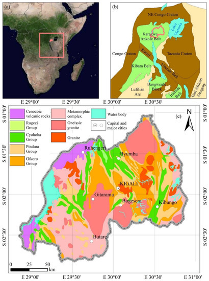
Figure 1.
(a) Location in central Africa (https://www.naturalearthdata.com/ and Tianditu); (b) geological setting (adapted from [46]); (c) regional geological map of Rwanda (adapted from [53]).
2.1.1. Stratums
The stratums in KAB are mainly composed of metasediment rocks and scarce carbonate rocks [46]. The earliest Kibaran lithosphere had subducted beneath the Tanzanian craton [43]. Mesoproterozoic stratums in Rwanda are defined as the Akanyaru Supergroup, which consists of four groups from bottom to top: Gikoro, Pindura, Cyohoha and Rugezi [37] (Figure 1c). Due to intensive tectonic events, the stratums are under various strikes.
2.1.2. Magmatic Rocks
The main magmatic events in Rwanda were S-type granitic intrusions, which were mainly triggered by probable lithospheric delamination and asthenospheric upwelling that provoked crustal melting (partial melt of the 2 Ga Rusizian metasedimentary basement [36]) during the subduction between the Congo and Tanzania cratons [43]. The granitic intrusions had developed four generations, including G1, G2, G3 (all gneissic) and G4 (i.e., tin granites, not gneissic). G1–G3 granites intruded at 1380 ± 10 Ma (U-Pb), and G4 granites took place around 986 ± 10 Ma (U-Pb) [36]. G4 granites are leuco granites characterized by equigranular, unfoliated alkali feldspars, muscovites, a spot of biotites and accessory minerals including apatite, tourmaline, ilmenite, monazite, xenotime and zircon [50,57]. Additionally, they are also enriched in Li, Rb, Cs, U and Sn elements [50].
Pegmatites and quartz veins in Rwanda are important ore-bearing geological bodies. Pegmatites are generally regarded as the products of differentiation of the evolved leucogranites [54] and are spatiotemporally associated with peraluminous G4 granites [47]. A regional pegmatite zonation 30 km west-southwest of the Nyakabingo deposit in Gatumba–Gitaramais was aged in 975 ± 8 Ma (U-Pb), and the Ar-Ar ages of muscovite samples vary between 940 Ma and 560 Ma, which suggests the Late Neoproterozoic tectonic thermal events [46]. Additionally, a close spatiotemporal relationship between Sn-quartz veins and early Neoproterozoic leucogranite and pegmatite intrusions was reported [36,56].
2.1.3. Structures
Structural deformation in Rwanda is complex and varies in dimensions. Regional anticlines and synclines can be identified on the geological map and remote sensing imagery, the axes of which are mainly NW- and NE-oriented. In general, the maximum stress seemed to be regionally EW-oriented during the compressive events, and the minimum stress was expected to be EW-oriented during the extensional relaxation [43].
2.2. Metallogenic Characteristics
2.2.1. Ore-Controlling Factors
The W, Sn, and Nb-Ta mineralization in Rwanda is characterized by Nb–Ta–Sn-pegmatite, W-quartz vein and Sn-quartz vein [48] and is spatiotemporally related to the G4 granites [53]. The W deposits in central Rwanda are related to carbonaceous shale, with bedding rocks serving as a reactive horizon [40]. W-bearing quartz veins in the Nyakabingo W deposit are located on the eastern flank of the Bumbogo anticline and are hosted in sandstones and black organic-rich metapelitic rocks [48]. The Sn-bearing quartz veins in the Musha Sn deposit and the pegmatites in the Ntunga Sn-Ta deposit are hosted in low-grade metamorphic pelites and meta-sandstones [44]. Sometimes, Sn-bearing quartz veins are hosted in muscovite-feldspar-rich sandstone and quartzite, and W-bearing quartz veins are hosted in organic-rich metapelites [48,58]. The analysis of Sn-quartz veins in the Rwamagana–Musha–Ntunga area indicated that the hydrothermal fluids consisted of 20%–95% magmatic fluids and 5%–80% metamorphic fluids [53]. Due to the bedding-parallel joints, interactions between fluids and stratums, and the involvement of metamorphic fluids, mineralization may tend to be stratum-selective.
From aerial photographs, the locations of mineral occurrences in Gatumba are strongly related to structural factors, indicating most of the deposits are associated with fractures [39]. W-bearing vein-type deposits in the “tungsten belt” (central Rwanda) are located in the core and along the flanks of secondary anticlines crosscut by numerous faults, some of which might act as pathways of fluids [40]. Tumukunde [43] and Dewaele [49] also regarded faults in Rutsiro as the main pathways for the emplacement of metal-rich fluids. Pegmatites adjacent to the mining field of Gatumba Mining Company occur along the cleavage planes [46]. Sn-Ta-bearing pegmatites in Musha–Ntunga are controlled by a regional NNW-SSE shear zone, 4 km west of a granite deposit [44]. Hulsbosch [45] considered that mineralization in Rwamagana–Musha–Ntunga (eastern Rwanda) was controlled by two factors: (1) reactivation of pre-existing discontinuities such as beddings, bedding-parallel joints or strike-slip fault planes, and (2) the regional post-compressional stress regime.
2.2.2. Mineral Alteration
In the Nyakabingo W-bearing vein deposit, mineralization took place with quartz and euhedral arsenopyrite, pyrite, scheelite, massive ferberite, and molybdenite [40]. The cassiterite mineralization is closely related with intense phyllic alterations, while the columbite-tantalite mineralization is followed by intense alkali metasomatism (the widespread existence of albite and white mica) [46]. The arsenopyrite, pyrite and pyrrhotite of W- and Sn-bearing vein deposits in Rutsiro imply at least one sulphide phase existed in later stages of W and Sn mineralization [43]. Illite is a common alteration product of feldspars found in ore deposits and mineralized zones [59], and goethite is a typical weathering product of pyrite. It can be seen from the above that W, Sn, and Nb-Ta mineralization might be indicated by the surface concentration of goethite-quartz, quartz, and illite, respectively.
3. Data and Methods
Figure 2 shows the RF-based framework of the regional quantitative MPM in this study, comprising three main parts: data processing, modeling, and prediction.
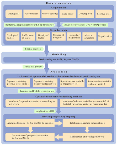
Figure 2.
Flowchart of regional quantitative MPM in this study.
3.1. Data Processing
Geological, geophysical, remote sensing, landcover, geographical, and mineralization data were collected during this study (Table 1). To process the data, firstly, regional geological map and faults in western Rwanda were facsimiled to obtain vectorized original data. Secondly, Bouguer samples and magnetic samples were interpolated to generate raster-format anomaly map. Thirdly, according to metallogenic characteristics, the digital original data were processed to generate secondary data, including: buffer zones of granites boundaries derived from regional geological map, a 1000m-upward map derived from a geophysical anomaly map, faults derived a from Bouguer 1000m-upward map, faults interpreted in eastern Rwanda from remote sensing imageries, buffer zones of faults, buffer zones of geographical elements, linear density map of faults, mineral alterations extracted from remote sensing, and negative sites of W, Sn, Nb, and Ta (Table 1). Finally, original data and secondary data together formed the relevant layers (Table 2, Figure 3). Specifically, buffer zones were generated via the “buffer” tool in ArcGIS, a 1000 m-upward map was processed by GeoIPAS software on the basis of anomaly map, and was classified into 5 area-equal ranges, Bouguer faults were visually interpreted from a Bouguer map upward of 1000 m according to the distribution of the linear gradient zone, convergence of contour [60], linear density maps were generated via the “line density” tool in ArcGIS, and were also classified into 5 area-equal ranges, and additionally geological faults in western Rwanda were collected from Uwiduhae [25]. The distribution of geological faults was approximately consistent with the Landsat 8 OLI imageries and ASTER GDEM. Hence, faults in eastern Rwanda were derived from true color image, false component image, and terrain via visual interpretation. Spatial analysis showed that the distance between two adjacent positive sites were less than 13 km, 10 km, 17 km for most of the positive W, Sn, and Nb-Ta sites, respectively. Thus, 13 km, 10 km, and 17 km buffer zones for W, Sn, and Nb-Ta were generated [28], and the negative sites for W, Sn, and Nb-Ta were created randomly out of the buffer zones.

Table 1.
List of data.
Table 2.
Relevant layers of W, Sn, and Nb-Ta mineralization in Rwanda.
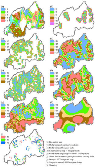
Figure 3.
Relevant layers involved in this study.
Rwanda is mainly covered by forest and cultivated land, making the extraction of mineral alteration very difficult. In order to reduce the influence of noise information, firstly, the Landsat 8 OLI imageries were masked by dense vegetation (NDVI exceeds 0.6), cultivated land, lakes, wetland, artificial surface, and 50 m buffer zones of roads and rivers. The masking left the residual valid pixels scattered in some regions of the imageries. Secondly, the directed principal component analysis (DPCA) method [31,32,33] was utilized to extract goethite, illite, and quartz alterations. This method aims to enhance mineral information by principal analysis between two band ratio images: one of these images contains information about hydrothermal alterations (band5/band7 for goethite, band5/band3 for illite, band5/band1 for quartz), the other image contains information of vegetation (band5/band4 for goethite, band3/band4 for illite, band5/band4 for quartz). Thirdly, to deal with the scattered distribution of alterations caused by the scattered distribution of residual pixels, this study proposed that an additional interpolation–density–delineation (IDD) process be performed on the extracted alteration map after the DPCA method. Seven main steps were included in the IDD process: (1) all the pixels in the original alteration map (i.e., Alteration map #1, Figure 4a) were converted into points (Figure 4b) in ArcGIS; (2) an alteration map #2 (Figure 4d) was generated via the “interpolation” tool on the points; (3) a corresponding point density map #1 (Figure 4c) was generated via the “point density” tool; (4) the range of the density map #1 (Figure 4c) was stretched to 0.5~1.0, namely point density map #2 (Figure 4f); (5) alteration map #3 (Figure 4e) was generated via the product of alteration map #2 (Figure 4d) and the point density map #2 (Figure 4f); (6) statistics of alteration map #3 (Figure 4e) were analyzed, and the lower limit of anomaly was determined by adding the mean value to 2.5 times the standard deviation (Figure 4h), and (7) the alteration map #4 (Figure 4g) was delineated along the anomaly of mean + 2.5 Stdev map (Figure 4h) to represent the distribution of a specific mineral alteration. Goethite, illite, and quartz alterations in Rwanda were obtained via the DPCA-IDD process (Figure 3i).
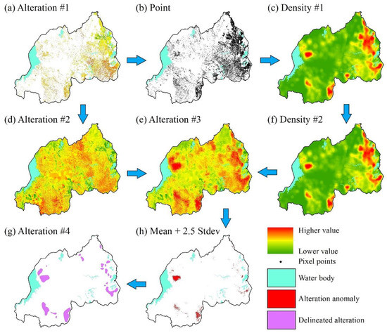
Figure 4.
Flowchart of the interpolation–density–delineation (IDD) process. (a) Alteration #1 map obtained by DPCA process; (b) Point map obtained in the 1st step; (c) Density #1 map obtained in the 3rd step; (d) Alteration #2 map obtained in the 2nd step; (e) Alteration #3 map obtained in the 5th step; (f) Density #2 map obtained in the 4th map; (g) Final alteration #4 map obtained in the 7th step; (h) Alteration #3 anomaly map in the 5th step.
3.2. Modeling
Mineralization refers to the formation of natural geological bodies with a single mineral (or multiple minerals) and a single genesis (or multiple geneses) in a specific time and geological setting [61]. Since different minerals with different geneses have various geological settings and ore-controlling factors, specific models should be established to identify the predictor layers and ensure the precision of MPM. Understanding the genesis and controlling factors of mineralization is the basis of MPM [62,63]. Mineralization processes in Rwanda include: (1) deposition of meta-sedimentary rocks; (2) intrusion of G1–G3 granites in an extensional context; (3) deposition of sediments, with deformation of 1000 Ma; (4) syn- to post-folding G4 granite intrusion; and (5) the intrusion of mineralized pegmatites and veins [51]. As mentioned before, the ore-forming G4 granite was emplaced around 986 Ma, indicating that the pegmatite-, vein-type W, Sn, and Nb-Ta mineralization in Rwanda could only be possible in geological bodies earlier than Neoproterozoic, and was selective for stratums and controlled by structures; in addition, the surface concentrations of goethite-quartz, quartz, and illite could partially be indicators for W, Sn, and Nb-Ta mineralization, respectively. Additionally, the geophysical field may change due to mineralization and the existence of ore-controlling factors.
The 3D mineral prospectivity software developed by the research team of Professor Jianping Chen, China University of Geosciences (Beijing), was employed to determine predictor layers on the basis of metallogeny and relevant layers. This software is capable of statistical analysis of the spatial relationships between the relevant layers and positive sites. The relevant layers containing a sufficient number of positive sites were identified as predictor layers for each mineral, finds which were summarized in the predictive model (Table 3, Table 4 and Table 5).
Table 3.
Predictive model of W mineralization in Rwanda.
Table 4.
Predictive model of Sn mineralization in Rwanda.
Table 5.
Predictive model of Nb-Ta mineralization in Rwanda.
Weights of evidence method was introduced to MPM by Agterberg [64], the weights of different predictor layers could be calculated according to spatial distributions between deposits and predictor layers, the algorithm is illustrated in Equation (1):
where DA and DB are the quantities of units with and without deposits, respectively, BA and BB are the quantities of units with and without a specific predictor layer I, respectively. P(BA/DA) is the probability of BA when DA is present in an unit, WI+ and WI− are the weights of I when I is present and absent in an unit, respectively. CI means Contrast, is an index of how well a predictor layer is related to deposits, and is designated as positive (I is advantageous to mineralization) or negative (disadvantageous).
In this study, weight of evidence method was employed to precheck the spatial contrasts of predictor layers (Table 6). Linear density, which describes the energy intensity of the tectonic activity, mainly had high spatial contrast (1.49, 1.41 for W, 1.03, 0.55 for Sn, 1.31, 1.02 for Nb-Ta); buffer zones of faults, which represent fracture zones, mainly possessed medium spatial contrast (0.99, 0.90 for W, 0.89, 0.53 for Sn, 1.74, 0.60 for Nb-Ta). The above indicates the considerable the ore-controlling effect of faults, which acted as reservoirs or pathways of hydrothermal fluids. As widely applied mineralization indicators, the distributions of Bouguer and magnetic anomalies are characterized by various underground geological bodies [60]. In this study, high–medium spatial contrasts (1.08, 0.83 for W, 1.14, 1.00 for Sn, 1.27, 1.09 for Nb-Ta) could be derived from lower Bouguer and medium magnetic anomalies, which covered the extent of granites. The buffer zones of granite boundaries also exhibited high–medium spatial contrasts (1.03 for W, 1.02 for Sn, 0.84 for Nb-Ta). Together with the high spatial contrast (1.53) of granite for Nb-Ta, they confirmed the existing metallogenic origin conclusions [36,47,53,54,56]. Stratums, which might help in the reaction of hydrothermal fluids [40], showed medium–low spatial contrast (0.60, 0.49, 0.21 for W, 0.71, 0.53, 0.25, 0.22 for Sn, 0.41, 0.35, 0.09 for Nb-Ta). The reason for this might be that the geological groups are too large to reflect the role of specific rocks [40,44,48,58] as reactive horizon. The alterations generally had lower spatial contrast (0.55, 0.37 for W, 0.06 for Sn, 0.62 for Nb-Ta) due to the relatively lower accuracy of alteration extraction caused by dense vegetation and cultivated land. However, the positive spatial contrasts of alterations verified the validation of the DPCA-IDD process.
Table 6.
Weights and Contrasts of predictor layers for W, Sn, and Nb-Ta mineralization.
3.3. Prediction
An ensemble learning machine (ELM) is a combination of individual learning machines and ensemble algorithms [65], and types of individual learning machines could be the same or different. Random forest (RF), proposed by Breiman [66], is a highly robust discrimination ELM comprised of a number of decision trees (i.e., classification and regression tree (CART)) that are organized hierarchically by a set of rules [67,68,69]. Characterized by bootstrapping, subsets of variables, and the integration of votes (Figure 5), RF is advantageous in accuracy and generalization ability. Bootstrapping means that each decision tree in RF uses a specific training subset, every sample in the training subset is randomly chosen from the total training dataset and then replaced [67], approximately 2/3 of samples (namely in bag samples) in the total training dataset are randomly chosen to train a specific decision tree, while 1/3 (namely out of bag samples, i.e., OOB) have never been chosen [70]. Though cross-validation or a separate test training dataset is not necessary as the OOB could be used as test data [1], McKay [70] used both 5-fold cross-validation and OOB errors to estimate the overall classification error. In common studies, positive and negative samples in k-fold cross-validation were not separately treated, leading to the numbers of positive and negative samples being random in every fold. Additionally, in order to reduce the imbalance between positive and negative samples in the k-fold cross-validation, a k2-fold cross-validation method was firstly introduced in this study. As the k2-fold cross-validation method proposed, positive and negative samples were k-folded separately, and every fold of positive and negative samples were combined into training and test training sets. The quantity of sets is k2, as seen if we take 52-fold as an example: the folds of positive sample include S+1, S+2, S+3, S+4, and S+5, the folds of negative sample include S−1, S−2, S−3, S−4, and S−5, and together they can combine into 25 training and test training sets (Table 7). Additionally, the total error is represented by the mean error of the 25 training and test training sets. A subset of variables means that for each node of a decision tree, a random selection of the input variables is made, then the best variable is chosen from the random selection of variables, and the size of random selection is a fraction of the total number of variables [70]. The integration of votes means that the final output of RF is based on the majority or mean of outputs from all decision trees [22,71]. RF has been proven effective for MPM [27], and performs well with fewer training sample sets [72]. As few as 14~16 positive sites were used in RF-based MPM for different districts with ideal results [22,70]. In MPM, the values of positive sites are always set to 1, while the negative sites are set to 0 [1]. For regression mission, the predictions are floating values ranging from 0 to 1, denoting likelihoods of deposits. For classification mission, the predictions can be categorized into prospective and non-prospective areas using a certain threshold value [67].
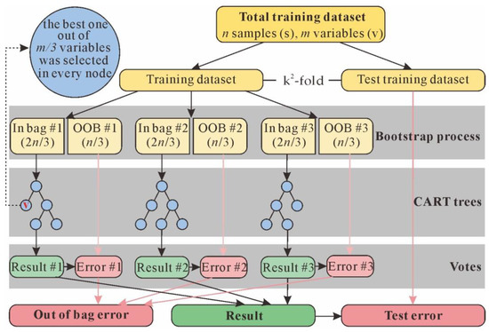
Figure 5.
Flowchart of RF algorithm (adapted from [1]).
Table 7.
Illustration of training and test training datasets of 52-fold cross-validation.
Model training is an important step to producing accurate predictions [16]. In this study, the “RF_MexStandalone_v0.02” package was applied to RF-based MPM. Firstly, approximately 26,000 1 × 1 km-sized squares were zoned in Rwanda, AND values of squares containing positive or negative sites were set to 1 or 0, respectively; squares where variables (i.e., predictor layers) were present or absent were set to 1 or 0, respectively. Secondly, a number of decision trees and number of selected variables for every node are prerequisite to running RF [73]. Errors always converge as the number of trees increase [74], and RF is less sensitive to the number of selected variables as the errors converge [1]. Hence, the number of selected variables was set to 1/3 of the total variables quantity as recommended [67]. The 52-fold cross-validation was utilized to divide the training dataset into training and test training subsets, and the accuracy of RFs with 50~1000 decision trees was trained and tested using the training and test training subsets, respectively, then, an optimal number of decision trees was determined according to the test error. Thirdly, the RF with optimal number of decision trees was applied to regress the likelihoods of W, Sn, and Nb-Ta deposit in each square, respectively. In addition, the total mineralization potential was calculated based on likelihoods of W, Sn, and Nb-Ta deposits (Equation (2)). Finally, metallogenic belts and prospective areas were delineated according to total mineralization potential and likelihoods of W, Sn, and Nb-Ta deposits, respectively.
where PT represents the total mineralization potential, LW represents the likelihood of W deposit, LSn represents the likelihood of Sn deposit, and LNb-Ta represents the likelihood of Nb-Ta deposit.
PT = (LW + LSn + LNb-Ta)/3
4. Results
4.1. Performance of RF
The parameter configuration of RF is of great influence on its generalization capacity and efficiency. Figure 6a shows the relationship between the test error and the number of trees, while the number of selected variables was set to 1/3 of the total variables quantity, as recommended [66]. From about 700 trees, the error stabilized around 0.268, 0.272, and 0.252 for W, Sn, and Nb-Ta mineralization, respectively, the fluctuation (ranges from 0 to 1) was less than 0.01. The addition of more trees neither decreased nor increased the error significantly, but increased the computation time, and hence 700 trees were set to the RF model.
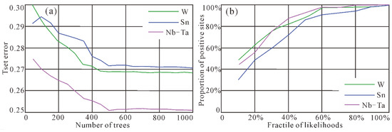
Figure 6.
(a) Test error curves and (b) capture–efficiency curves of the RF model.
Capture–efficiency curves were derived to evaluate the performance of the RF models of W, Sn, and Nb-Ta mineralization, respectively. The curve was obtained as follows: firstly, all the likelihoods of squares in Rwanda were ranked from the highest to the lowest, and 10-fractiles of squares were calculated; secondly, the quantities of positive sites (Sp) out of the total positive sites (ST) linked with the top 10%, 20%,…,100% squares were recorded; finally, the proportion of positive sites (Sp/ST) within the top 10%, 20%,…,100% squares was calculated. Figure 6b shows the derived capture–efficiency curves of the RF model, where the x axis represents the fractiles of squares and the y axis represents the proportion of positive sites. As we can see, approximately 90% of the positive sites are linked with the top 50% squares with the highest likelihoods from RF modeling. In general, the RF model for Nb-Ta has the best performance. These results also indicate that the RF model has produced a reasonable probability distribution, with predictor layers totally derived from open source data on the website.
4.2. Metallogenic Belts and Prospective Areas
Metallogenic belts could be categorized into 5 levels, among which the I-level is equal to a global-scale region, II-level is equal to one or several tectonic elements, III-level refers to a region where mineralization was formed or controlled by the same geological activities, IV-level refers to the sub-belt of III-level, and V-level refers to the ore field [75]. As we know, Rwanda as a whole is under the same metallogenesis conditions. Hence, seven IV-level metallogenic belts were delineated according to the distribution of total mineralization potential and regional geology (Figure 7a). Belt IV-1, with a mean total mineralization potential of 0.4526, is located in eastern Rwanda and possesses a Cyohoha group, a Pindura group, and a Gikoro group in the west and a metamorphic complex in the east, and there are also granites in the middle and north; faults are mainly NNE- and SN-oriented, regional anticline could be identified in the middle-west (Figure 7b, Table 8), and several positive sites were discovered near the anticline (Figure 7a). Belt IV-2, with a mean total mineralization potential of 0.4559, located in middle-eastern Rwanda, mainly possesses a Gikoro group in the south, and there are gneissic granites in the north and granites in the middle; NNW-oriented faults mainly exist in the Gikoro group. There are also NE-oriented faults in the gneissic granites (Figure 7b, Table 8), and a number of positive sites were discovered adjacent to the granites (Figure 7a). Belt IV-3, with a mean total mineralization potential of 0.4925, located in central Rwanda, possesses a Cyohoha group, a Pindura group, and a Gikoro group in the north and middle, and there are also granites in the middle; faults are mainly NNW-oriented, followed by the NE-facing ones, the regional anticline could be identified in the middle (Figure 7b, Table 8), and a number of positive sites were discovered along the granites and the regional anticline (Figure 7a). Belt IV-4, with the best mean total mineralization potential of 0.6013, is located in northwestern Rwanda; it possesses a Cyohoha group and a Gikoro group in the east and metamorphic complex in the west, and there are granites in the middle and gneissic granites in the west of the belt; faults are mainly SN-oriented (Figure 7b, Table 8), and a great amount of positive sites were discovered in the middle and west (Figure 7a). Belt IV-5, with the lowest mean total mineralization potential of 0.2899, located in southwestern Rwanda, mainly possesses the Cyohoha group in the north and metamorphic complex in the south, and there are large-scale gneissic granite deposits in the middle; faults are mainly NNW-, NNE-oriented, and exist along the boundaries of gneissic granite (Figure 7b, Table 8). In addition, no positive sites were found in this belt (Figure 7a). Belt IV-6, with a mean total mineralization potential of 0.3295, located in southwestern Rwanda, mainly possesses the metamorphic complex, followed by Cyohoha group, Gikoro group in the east and scattered Pindura group, and there are granites in the northwest and gneissic granites in the middle; faults are mainly NW- and SN-oriented (Figure 7b, Table 8), several positive sites were discovered in the north and south (Figure 7a). Belt IV-7, with a mean total mineralization potential of 0.3223, located in western Rwanda, possesses a Cyohoha group, a Pindura group, and Gikoro group in the east and Cenozoic volcanic rock in the west; faults are mainly NNW-, NNE-oriented (Figure 7b, Table 8), only one W site was found near Belt IV-6 (Figure 7a).
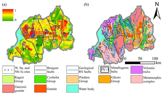
Figure 7.
(a) Total mineralization potential and (b) geological characteristics of metallogenic belts. This figure was changed.
Table 8.
Attributes of metallogenic belts.
The top 10%, 20%, and 30% of squares were classified as higher, medium, and lower likelihood regions, respectively (Figure 8). Prospective areas for W, Sn, Nb-Ta were delineated along the boundaries of higher likelihood regions within metallogenic belts, and they were graded into A-, B-, and C-levels according to positive sites, spatial continuity, the mean likelihood of deposits, and areas. As the achievements of this mapping activity, 2 A-level, 2 B-level, and 7 C-level prospective areas for W (Figure 8a), 3 A-level, 3 B-level, and 11 C-level prospective areas for Sn (Figure 8b), 3 A-level, 3 B-level, and 5 C-level prospective areas for Nb-Ta (Figure 8c) were finally delineated. These are mainly located in the middle-west (IV-4) and east (IV-2, IV-1) of Rwanda (Figure 8, Table 9, Table 10 and Table 11).

Figure 8.
Prospective areas of W, Sn, and Nb-Ta in Rwanda. This figure was changed. (a) Prospective areas of W mineralization; (b) Prospective areas of Sn mineralization; (c) Prospective areas of Nb-Ta mineralization.
Table 9.
Attributes of W prospective areas.
Table 10.
Attributes of Sn prospective areas.
Table 11.
Attributes of Nb-Ta prospective areas.
Some target areas were delineated by previous studies via the interpretation of aeromagnetic data in western Rwanda [25]. Comparing metallogenic belts and prospective areas in this study and target areas in previous study, two out of six target areas are located in Belt IV-4, while three out of six target areas are located in Belt IV-6, showing a partially consistency. Prospective areas W-A2-2, W-B2-1, W-C7-4, Sn-A3-1, Sn-A3-3, Sn-B3-1, NbTa-A3-1, NbTa-B3-1, NbTa-B3-2, and NbTa-C5-2, which are mainly located in Belt IV-4, are partially consistent with the target areas. The comparison also shows that the total mineralization potential of Belt IV-4 is robust. A difference between previous study and this study might be caused by two reasons: (1) the previous study was knowledge-driven, and was solely conducted via high-resolution magnetic anomaly data, while this study was data-driven, and was conducted via integrated open source data analysis; (2) the previous study was conducted in western Rwanda, which would only highlight the areas with relatively high mineralization potential in west part of the country, while this study was conducted in the whole country, so areas with higher mineralization potential in the middle-eastern Rwanda, rather than in the southwestern Rwanda, were delineated.
5. Discussion
To demonstrate the feasibility of drawing a prospectivity map using predictor layers derived from open source data, this study generated a series of secondary data, including faults, a density map of faults, a upward map of geophysical anomalies, and mineral alteration data. Then, RF models with 700 regression trees were applied to conduct the MPM process, in which known positive and negative sites were set to 1 and 0, respectively. This means that the final prospectivity map also ranges from 0 to 1, and a greater value represents better likelihood of deposits. The accuracy of RF models using open source data were represented by test errors with 25 training and test-training sets (i.e., 52-fold cross-validation). Results showed that the errors were around 0.268, 0.272, and 0.252 for W, Sn, and Nb-Ta MPM, respectively (Figure 6a), and approximately 90% of the positive sites were covered by the top 50% squares with the highest likelihoods (Figure 6b). Comparing to the recent MPM using sufficient and detailed data [1,16,24,28], the performances of MPM in this study using open source data were not ideal, but they proved the validation of open source data in regional quantitative MPM, helped to get a big picture of mineralization potential, and additionally identified preliminary prospect in the study area.
The masking of dense vegetation during remotely sensed mineral alteration extraction may provide researchers with fragmented imageries. However, alteration maps generated from these imageries, with many blank (masked) areas, are short in reliability and legibility. In order to reduce the negative effects of blank areas, the additional interpolation–density–delineation (IDD) process on the extracted alteration map was proposed. The IDD process fills the masked areas via interpolation, and the reliability of the interpolated map is assessed by the pixel density map. The range of the density map was then stretched to 0.5~1.0 to represent the transfer from the former blank area to the intact area, respectively, then, a new alteration map was reconstructed with the product of the interpolated alteration map and density map. To avoid interference pixels (e.g., sand beach along rivers) which survived from masking and may cause unreasonable alteration distributions, the use of manual delineation was recommended to generate the final alteration map. In this study, goethite, illite, and quartz alterations in Rwanda (Figure 3i) were obtained through the DPCA-IDD process. Acceptable contrasts were shown, except for the quartz alteration in the Sn MPM (with a contrast of 0.06). This might be explained by the concurrence of Nb-Ta-Sn pegmatite and an Sn quartz vein [48], and the contrast between quartz and Sn mineralization was drawn back by the Sn preserved in pegmatites.
As seen from Figure 7a, Belt IV-4, with a large set of W, Sn, and Nb-Ta deposits and the best mean mineralization potential (Table 8), mainly possesses A-, and B-level prospective areas; while B-, and C-level prospective areas take the lead in the IV-2, IV-1, and other belts, these are consistent with the principle of data driven MPM: more deposits indicate better metallogenic conditions. Mineral mining in Rwanda is conducted mainly as artisanal and small-scale mining [76], indicating that the ore bodies may be primarily explored near the surface, and that reserves are relatively less exploited. Hence, there is a high likelihood in A-level prospective areas with deposits are still not out of date. Additional mineral exploration is firstly recommended along and under the known deposits in A-level areas, while the B-, and C-level prospective areas may act as long-term reserves for future pursuing.
6. Conclusions
In this paper, regional quantitative MPM using integrated information was carried out to fill the void in mineral prospecting and exploration studies. To conduct this prospectivity study, open source data were taken full advantage of, including geological maps in the literature, gravity anomaly, magnetic anomaly, remote sensing, and other geographical information. Multispectral imageries are still easily available and important data source for mineral exploration. Landsat 8 OLI imageries were applied to identify faults and extract mineral alterations in Rwanda through visual interpretation and the DPCA-IDD process, respectively. The 2 km buffer zones and high densities of geological remote sensing faults exhibited medium to high contrast with known deposits, while mineral alterations mainly possessed medium contrast (Table 6). From the results of this paper, the MPM process turned out to be valid, and the metallogenic belts and prospective areas helped to understand the potential and pattern of W, Sn, Nb-Ta mineralization in Rwanda, which is worth understanding. Additionally, the IDD process is a suitable method for acquiring a spatially continuous alteration map from masked imageries, although the manual delineation process in IDD may cause subjective results. Reducing interference pixels through masking should be paid more attention, because reducing interference pixels could further reduce the unreasonably distribution of alterations and the necessity of manual delineation. In addition, the k2-fold cross-validation could provide more reasonable testing errors than the k-fold cross-validation.
Author Contributions
Conceptualization, Z.C. and J.C.; methodology, Z.C. and J.C.; software, Z.C. and Q.Y.; writing—original draft preparation, Z.C. and J.C.; writing—review and editing, Z.C. and J.C.; visualization, Z.C., T.L., Y.L., Q.Y. and H.D.; funding acquisition, T.L. All authors have read and agreed to the published version of the manuscript.
Funding
This research was funded by Harbin Center for Integrated Natural Resources Survey, China Geological Survey, and China University of Geosciences (Beijing).
Data Availability Statement
The complete spherical Bouguer gravity anomaly is openly available at http://bgi.obs-mip.fr/data-products/grids-and-models/wgm2012-global-model/. The earth magnetic anomaly grid is openly available at https://www.ncei.noaa.gov/products/earth-magnetic-model-anomaly-grid-2. The Landsat 8 imageries are openly available at https://earthexplorer.usgs.gov/. The DEM are openly available at https://www.gscloud.cn/search. The Globeland30 are openly available at http://www.globallandcover.com/. Additionally, the roads and rivers data are openly available at https://data.maptiler.com/downloads/dataset/osm/africa/rwanda/#11.07/-1.9756/29.8315.
Acknowledgments
The authors thank anonymous reviewers for their constructive comments and instructions, and editors for their elaborative, patient assistances. The authors would also like to acknowledge Bureau Gravimetrique International, National Oceanic and Atmospheric Administration, U.S. Geological Survey, Geospatial Data Cloud, Globeland30, and OpenStreetMap for providing access to geophysical, remote sensing, DEM, landcover, and geographical dataset, which were the foundation of this study.
Conflicts of Interest
The authors declare no conflict of interest.
References
- Rodriguez-Galiano, V.F.; Chica-Olmo, M.; Chica-Rivas, M. Predictive modelling of gold potential with the integration of multisource information based on random forest: A case study on the Rodalquilar area, Southern Spain. Int. J. Geogr. Inf. Sci. 2014, 28, 1336–1354. [Google Scholar] [CrossRef]
- Cargill, S.M.; Clark, A.L. Report on the activity of IGCP Project 98. J. Int. Assoc. Math. Geol. 1978, 10, 411–417. [Google Scholar] [CrossRef]
- Xiang, J.; Xiao, K.; Carranza, E.J.M.; Chen, J.; Li, S. 3D mineral prospectivity mapping with random forests: A case study of Tongling, Anhui, China. Nat. Resour. Res. 2020, 29, 395–414. [Google Scholar] [CrossRef]
- Yin, J.; Li, N. Ensemble learning models with a Bayesian optimization algorithm for mineral prospectivity mapping. Ore Geol. Rev. 2022, 145, 104916. [Google Scholar] [CrossRef]
- Silva dos Santos, V.; Gloaguen, E.; Hector Abud Louro, V.; Blouin, M. Machine learning methods for quantifying uncertainty in prospectivity mapping of magmatic-hydrothermal gold deposits: A case study from Juruena mineral province, northern Mato Grosso, Brazil. Minerals 2022, 12, 941. [Google Scholar] [CrossRef]
- Zuo, R.; Carranza, E.J.M. Support vector machine: A tool for mapping mineral prospectivity. Comput. Geosci. 2011, 37, 1967–1975. [Google Scholar] [CrossRef]
- Rodriguez-Galiano, V.F.; Sanchez-Castillo, M.; Chica-Olmo, M.; Chica-Rivas, M. Machine learning predictive models for mineral prospectivity: An evaluation of neural networks, random forest, regression trees and support vector machines. Ore Geol. Rev. 2015, 71, 804–818. [Google Scholar] [CrossRef]
- Mao, X.; Zhang, W.; Liu, Z.; Ren, J.; Bayless, R.C.; Deng, H. 3D mineral prospectivity modeling for the low-sulfidation epithermal gold deposit: A case study of the axi gold deposit, western Tianshan, NW China. Minerals 2020, 10, 233. [Google Scholar] [CrossRef]
- Fu, C.; Chen, K.; Yang, Q.; Chen, J.; Wang, J.; Liu, J.; Xiang, Y.; Li, Y.; Rajesh, H.M. Mapping gold mineral prospectivity based on weights of evidence method in southeast Asmara, Eritrea. J. Afr. Earth Sci. 2021, 176, 104143. [Google Scholar] [CrossRef]
- Liu, L.; Lu, J.; Tao, C.; Liao, S. Prospectivity mapping for magmatic-related seafloor massive sulfide on the mid-Atlantic Ridge applying weights-of-evidence method based on GIS. Minerals 2021, 11, 83. [Google Scholar] [CrossRef]
- Carranza, E.J.M.; Laborte, A.G. Data-driven predictive mapping of gold prospectivity, Baguio district, Philippines: Application of Random Forests algorithm. Ore Geol. Rev. 2015, 71, 777–787. [Google Scholar] [CrossRef]
- Xiong, Y.; Zuo, R. GIS-based rare events logistic regression for mineral prospectivity mapping. Comput. Geosci. 2018, 111, 18–25. [Google Scholar] [CrossRef]
- Zhao, X.; Teng, S.; Lei, S. Mineral resources evaluation model research based on PSO algorithm and BP neural network. J. Inf. Comput. Sci. 2015, 12, 6257–6266. [Google Scholar] [CrossRef]
- Zhang, N.; Zhou, K.; Li, D. Back-propagation neural network and support vector machines for gold mineral prospectivity mapping in the Hatu region, Xinjiang, China. Earth Sci. Inform. 2018, 11, 553–566. [Google Scholar] [CrossRef]
- Sun, T.; Li, H.; Wu, K.; Chen, F.; Zhu, Z.; Hu, Z. Data-driven predictive modelling of mineral prospectivity using machine learning and deep learning methods: A case study from Southern Jiangxi Province, China. Minerals 2020, 10, 102. [Google Scholar] [CrossRef]
- Wang, K.; Zheng, X.; Wang, G.; Liu, D.; Cui, N. A multi-model ensemble approach for gold mineral prospectivity mapping: A case study on the Beishan region, western China. Minerals 2020, 10, 1126. [Google Scholar] [CrossRef]
- Li, T.; Xia, Q.; Zhao, M.; Gui, Z.; Leng, S. Prospectivity mapping for tungsten polymetallic mineral resources, Nanling metallogenic belt, south China: Use of random forest algorithm from a perspective of data imbalance. Nat. Resour. Res. 2020, 29, 203–227. [Google Scholar] [CrossRef]
- Xu, Y.; Li, Z.; Xie, Z.; Cai, H.; Niu, P.; Liu, H. Mineral prospectivity mapping by deep learning method in Yawan-Daqiao area, Gansu. Ore Geol. Rev. 2021, 138, 104316. [Google Scholar] [CrossRef]
- Li, S.; Chen, J.; Liu, C.; Wang, Y. Mineral prospectivity prediction via convolutional neural networks based on geological big data. J. Earth Sci. 2021, 32, 327–347. [Google Scholar] [CrossRef]
- Kong, Y.; Chen, G.; Liu, B.; Xie, M.; Yu, Z.; Li, C.; Wu, Y.; Gao, Y.; Zha, S.; Zhang, H. 3D mineral prospectivity mapping of Zaozigou gold deposit, west Qinling, China: Machine learning-based mineral prediction. Minerals 2022, 12, 1361. [Google Scholar] [CrossRef]
- Porwal, A.; Carranza, E.M.J. Introduction to the special issue: GIS-based mineral potential modelling and geological data analyses for mineral exploration. Ore Geol. Rev. 2015, 71, 477–483. [Google Scholar] [CrossRef]
- Ford, A. Practical implementation of random forest-based mineral potential mapping for porphyry Cu—Au mineralization in the eastern Lachlan Orogen, NSW, Australia. Nat. Resour. Res. 2019, 29, 267–283. [Google Scholar] [CrossRef]
- Zuo, R. Geodata science-based mineral prospectivity mapping: A review. Nat. Resour. Res. 2020, 29, 3415–3424. [Google Scholar] [CrossRef]
- Zhang, S.; Carranza, E.J.M.; Xiao, K.; Wei, H.; Yang, F.; Chen, Z.; Li, N.; Xiang, J. Mineral prospectivity mapping based on isolation forest and random forest: Implication for the existence of spatial signature of mineralization in outliers. Nat. Resour. Res. 2021, 31, 1981–1999. [Google Scholar] [CrossRef]
- Uwiduhae, J.D.; Claude Ngaruye, J.; Saibi, H. Defining potential mineral exploration targets from the interpretation of aeromagnetic data in Western Rwanda. Ore Geol. Rev. 2020, 128, 103927. [Google Scholar] [CrossRef]
- Yu, Z.; Liu, B.; Xie, M.; Wu, Y.; Kong, Y.; Li, C.; Chen, G.; Gao, Y.; Zha, S.; Zhang, H.; et al. 3D mineral prospectivity mapping of Zaozigou gold deposit, west Qinling, China: Deep learning-based mineral prediction. Minerals 2022, 12, 1382. [Google Scholar] [CrossRef]
- Zhang, Q.; Chen, J.; Xu, H.; Jia, Y.; Chen, X.; Jia, Z.; Liu, H. Three-dimensional mineral prospectivity mapping by XGBoost modeling: A case study of the Lannigou gold deposit, China. Nat. Resour. Res. 2022, 31, 1135–1156. [Google Scholar] [CrossRef]
- Daviran, M.; Maghsoudi, A.; Ghezelbash, R.; Pradhan, B. A new strategy for spatial predictive mapping of mineral prospectivity: Automated hyperparameter tuning of random forest approach. Comput. Geosci. 2021, 148, 104688. [Google Scholar] [CrossRef]
- Frutuoso, R.; Lima, A.; Teodoro, A.C. Application of remote sensing data in gold exploration: Targeting hydrothermal alteration using Landsat 8 imagery in northern Portugal. Arab. J. Geosci. 2021, 14, 459. [Google Scholar] [CrossRef]
- Pour, A.B.; Zoheir, B.; Pradhan, B.; Hashim, M. Editorial for the special issue: Multispectral and hyperspectral remote sensing data for mineral exploration and environmental monitoring of mined areas. Remote Sens. 2021, 13, 519. [Google Scholar] [CrossRef]
- Carranza, E.J.M.; Hale, M. Mineral imaging with Landsat thematic mapper data for hydrothermal alteration mapping in heavily vegetated terrane. Int. J. Remote Sens. 2002, 23, 4827–4852. [Google Scholar] [CrossRef]
- Fraser, S.J.; Green, A.A. A software defoliant for geological analysis of band ratios. Int. J. Remote Sens. 1987, 8, 525–532. [Google Scholar] [CrossRef]
- Shevyrev, S.; Carranza, E.J.M. Application of maximum entropy for mineral prospectivity mapping in heavily vegetated areas of Greater Kurile Chain with Landsat 8 data. Ore Geol. Rev. 2022, 142, 104758. [Google Scholar] [CrossRef]
- Chakraborty, R.; Kereszturi, G.; Pullanagari, R.; Durance, P.; Ashraf, S.; Anderson, C. Mineral prospecting from biogeochemical and geological information using hyperspectral remote sensing—Feasibility and challenges. J. Geochem. Explor. 2022, 232, 106900. [Google Scholar] [CrossRef]
- Rossetti, F.; Cozzupoli, D.; Phillips, D. Compressional reworking of the East African Orogen in the Uluguru Mountains of eastern Tanzania at 550 Ma: Implications for the final assembly of Gondwana. Terra Nova 2008, 20, 59–67. [Google Scholar] [CrossRef]
- Tack, L.; Wingate, M.T.D.; De Waele, B.; Meert, J.; Belousova, E.; Griffin, B.; Tahon, A.; Fernandez-Alonso, M. The 1375Ma “Kibaran event” in Central Africa: Prominent emplacement of bimodal magmatism under extensional regime. Precambrian Res. 2010, 180, 63–84. [Google Scholar] [CrossRef]
- Fernandez-Alonso, M.; Cutten, H.; De Waele, B.; Tack, L.; Tahon, A.; Baudet, D.; Barritt, S.D. The Mesoproterozoic Karagwe-Ankole Belt (formerly the NE Kibara Belt): The result of prolonged extensional intracratonic basin development punctuated by two short-lived far-field compressional events. Precambrian Res. 2012, 216–219, 63–86. [Google Scholar] [CrossRef]
- Debruyne, D.; Hulsbosch, N.; Wilderode, J.V.; Balcaen, L.; Vanhaecke, F.; Muchez, P. Regional geodynamic context for the Mesoproterozoic Kibara belt (KIB) and the Karagwe-Ankole belt: Evidence from geochemistry and isotopes in the KIB. Precambrian Res. 2015, 264, 82–97. [Google Scholar] [CrossRef]
- Dewaele, S.; Tack, L.; Fernandez-Alonso, M.; Boyce, A.; Muchez, P.; Schneider, J.; Cooper, G.; Wheeler, K. Geology and mineralisation of the Gatumba area, Rwanda: Present state of knowledge. Etudes Rwandaises 2008, 16, 6–24. [Google Scholar]
- Goldmann, S.; Melcher, F.; Gäbler, H.-E.; Dewaele, S.; De Clercq, F.; Muchez, P. Mineralogy and trace element chemistry of ferberite/reinite from Tungsten deposits in central Rwanda. Minerals 2013, 3, 121–144. [Google Scholar] [CrossRef]
- Hulsbosch, N.; Hertogen, J.; Dewaele, S.; Andre, L.; Muchez, P. Petrographic and mineralogical characterisation of fractionated pegmatites culminating in the Nb-Ta-Sn pegmatites of the Gatumba area (western Rwanda). Geol. Belg. 2013, 16, 105–117. [Google Scholar]
- Pohl, W.L.; Biryabarema, M.; Lehmann, B. Early Neoproterozoic rare metal (Sn, Ta, W) and gold metallogeny of central Africa: A review. Appl. Earth Sci. 2013, 122, 66–82. [Google Scholar] [CrossRef]
- Tumukunde, T.D.; Piestrzynski, A. Vein-type tungsten deposits in Rwanda, Rutsiro area of the Karagwe-Ankole Belt, central Africa. Ore Geol. Rev. 2018, 102, 505–518. [Google Scholar] [CrossRef]
- Goodship, A.; Dace, A.; O’Hare, P.; Uwiringiyimana, J.; Siddle, R.; Moon, C. Geology and genesis of the Musha-NtungaSn-Ta-Li-Nb vein-pegmatite deposit, Rwanda: First results from deep drilling of a coltan mine in Rwanda and first detailed description of Li minerals. Appl. Earth Sci. 2019, 128, 47–48. [Google Scholar] [CrossRef]
- Hulsbosch, N.; Van Daele, J.; Reinders, N.; Dewaele, S.; Jacques, D.; Muchez, P. Structural control on the emplacement of contemporaneous Sn-Ta-Nb mineralized LCT pegmatites and Sn bearing quartz veins: Insights from the Musha and Ntunga deposits of the Karagwe-Ankole Belt, Rwanda. J. Afr. Earth Sci. 2017, 134, 24–32. [Google Scholar] [CrossRef]
- Dewaele, S.; Henjes-Kunst, F.; Melcher, F.; Sitnikova, M.; Burgess, R.; Gerdes, A.; Fernandez, M.A.; De Clercq, F.; Mucheze, P.; Lehmann, B. Late Neoproterozoic overprinting of the cassiterite and columbite–tantalite bearing pegmatites of the Gatumba area, Rwanda (central Africa). J. Afr. Earth Sci. 2011, 61, 10–26. [Google Scholar] [CrossRef]
- Hulsbosch, N.; Hertogen, J.; Dewaele, S.; Andre, L.; Muchez, P. Alkali metal and rare earth element evolution of rock-forming minerals from the Gatumba area pegmatites (Rwanda): Quantitative assessment of crystal-melt fractionation in the regional zonation of pegmatite groups. Geochim. Cosmochim. Acta 2014, 132, 349–374. [Google Scholar] [CrossRef]
- Hulsbosch, N.; Boiron, M.C.; Dewaele, S.; Muchez, P. Fluid fractionation of tungsten during granite–pegmatite differentiation and the metal source of peribatholitic W quartz veins: Evidence from the Karagwe-Ankole Belt (Rwanda). Geochim. Cosmochim. Acta 2016, 175, 299–318. [Google Scholar] [CrossRef]
- Dewaele, S.; De Clercq, F.; Hulsbosch, N.; Piessens, K.; Boyce, A.; Burgess, R.; Muchez, P. Genesis of the vein-type tungsten mineralization at Nyakabingo (Rwanda) in the Karagwe-Ankole belt, Central Africa. Miner. Depos. 2016, 51, 283–307. [Google Scholar] [CrossRef]
- Lehmann, B.; Lavreau, J. Geochemistry of tin granites from Kivu (Zaire), Rwanda and Burundi. IGCP 255 Newsl. 1998, 1, 43–46. [Google Scholar]
- Ngaruye, J.C. Petrographic and Geochemical Investigation of Sn-W-Nb-Ta-Pegmatites and Mineralized Quartz Veins in Southeastern Rwanda. Ph.D. Thesis, University of the Free State, Bloemfontein, South Africa, 2011. [Google Scholar]
- Lehmann, B.; Halder, S.; Munana, J.R.; Ngizimanac, J.d.l.P.; Biryabarema, M. The geochemical signature of rare-metal pegmatites in central Africa: Magmatic rocks in the Gatumba tin–tantalum mining district, Rwanda. J. Geochem. Explor. 2014, 144, 528–538. [Google Scholar] [CrossRef]
- Van Daele, J.; Hulsboscha, N.; Dewaele, S.; Boiron, M.C.; Piessense, K.; Boyce, A.; Muchez, P. Mixing of magmatic-hydrothermal and metamorphic fluids and the origin of peribatholitic Sn vein-type deposits in Rwanda. Ore Geol. Rev. 2018, 101, 481–501. [Google Scholar] [CrossRef]
- Hulsbosch, N.; Muchez, P. Tracing fluid saturation during pegmatite differentiation by studying the fluid inclusion evolution and multiphase cassiterite mineralisation of the Gatumba pegmatite dyke system (NW Rwanda). Lithos 2019, 354–355, 109285. [Google Scholar] [CrossRef]
- Zhang, R.; Sun, W.; Lehmann, B.; Seltmann, R.; Li, C. Multiple tin mineralization events in Africa: Constraints by in-situ LA-ICPMS cassiterite U-Pb ages. In Proceedings of the 35th International Geological Congress, Cape Town, South Africa, 27 August–4 September 2016. [Google Scholar]
- Dewaele, S.; Hulsbosch, N.; Cryns, Y.; Boyce, A.; Burgess, R.; Muchez, P. Geological setting and timing of the world-class Sn, Nb-Ta and Li mineralization of Manono-Kitotolo (Katanga, Democratic Republic of Congo). Ore Geol. Rev. 2016, 72, 373–390. [Google Scholar] [CrossRef]
- Pohl, W.L. Metallogeny of the northeastern Kibarabelt, Central Africa—Recent perspectives. Ore Geol. Rev. 1994, 9, 105–130. [Google Scholar] [CrossRef]
- De Clercq, F. Metallogenesis of Sn and W Vein-Type Deposits in the Karagwe-Ankole Belt (Rwanda). Ph.D. Thesis, Katholieke Universitei Leuven, Leuven, Belgium, 2012. [Google Scholar]
- Meyer, J.M.; Kokaly, R.F.; Holley, E. Hyperspectral remote sensing of white mica: A review of imaging and point-based spectrometer studies for mineral resources, with spectrometer design considerations. Remote Sens. Environ. 2022, 275, 113000. [Google Scholar] [CrossRef]
- Liu, L. Application of Gravity Data Processing and Interpretation Technology in Geological Structure Interpretation and Mineral Prediction in Southern Tibet. Ph.D. Thesis, China University of Geosciences (Beijing), Beijing, China, 2021. (In Chinese with English abstract). [Google Scholar] [CrossRef]
- Chen, Y.; Pei, R.; Wang, D.; Huang, F. Minerogenetic series for mineral deposits: Discussion on minerogenetic series (V). Acta Geosci. Sin. 2016, 37, 519–527. [Google Scholar] [CrossRef]
- Hagemann, S.G.; Lisitsin, V.; Huston, D.L. Mineral system analysis: Quovadis. Ore Geol. Rev. 2016, 76, 504–522. [Google Scholar] [CrossRef]
- Xiao, K.; Xiang, J.; Fan, M.; Xu, Y. 3D mineral prospectivity mapping based on deep metallogenic prediction theory: A case study of the Lala copper mine, Sichuan, China. J. Earth Sci. 2021, 32, 348–357. [Google Scholar] [CrossRef]
- Agterberg, F.P.; Bonham-Carter, G.F.; Cheng, Q.; Wright, D.F. Weights of evidence modeling and weighted logistic regression for mineral potential mapping. In Computers in Geology: 25 Years of Progress; Davis, J.C., Herzfeld, U.C., Eds.; Oxford University Press: New York, NY, USA, 1993; pp. 13–32. [Google Scholar] [CrossRef]
- Zhou, Z. Machine Learning; Tsinghua University Press: Beijing, China, 2016; pp. 171–185. (In Chinese) [Google Scholar]
- Breiman, L. Random forests. Mach. Learn. 2001, 45, 5–32. [Google Scholar] [CrossRef]
- Carranza, E.J.M.; Laborte, A.G. Random forest predictive modeling of mineral prospectivity with small number of prospects and data with missing values in Abra (Philippines). Comput. Geosci. 2015, 74, 60–70. [Google Scholar] [CrossRef]
- Qin, Y.; Wu, W.; Xie, L.; Ou, P.; Huang, X. Application of machine learning based mineral prospectivity mapping in the Yuexi antimony orefield, Hunan province. J. East China Univ. Technol. 2021, 44, 28–40. [Google Scholar]
- Wang, S.; Zhou, K.; Wang, J.; Zhao, J. Identifying and mapping alteration minerals using HySpex airborne hyperspectral data and random forest algorithm. Front. Earth Sci. 2022, 10, 871529. [Google Scholar] [CrossRef]
- McKay, G.; Harris, J.R. Comparison of the data-driven random forests model and a knowledge-driven method for mineral prospectivity mapping: A case study for gold deposits around the Huritz group and Nueltin suite, Nunavut, Canada. Nat. Resour. Res. 2016, 25, 125–143. [Google Scholar] [CrossRef]
- Carranza, E.J.M.; Laborte, A.G. Data-driven predictive modeling of mineral prospectivity using random forests: A case study in Catanduanes Island (Philippines). Nat. Resour. Res. 2016, 25, 35–50. [Google Scholar] [CrossRef]
- Demarchi, L.; Canters, F.; Cariou, C.; Licciardi, G.; Chan, J.C.W. Assessing the performance of two unsupervised dimensionality reduction techniques on hyperspectral APEX data for high resolution urban land-cover mapping. ISPRS J. Photogramm. Remote Sens. 2014, 87, 166–179. [Google Scholar] [CrossRef]
- Parsa, M.; Maghsoudi, A. Assessing the effects of mineral systems-derived exploration targeting criteria for random forests-based predictive mapping of mineral prospectivity in Ahar-Arasbaran area, Iran. Ore Geol. Rev. 2021, 138, 104399. [Google Scholar] [CrossRef]
- Breiman, L. Bagging predictors. Mach. Learn. 1996, 24, 123–140. [Google Scholar] [CrossRef]
- Song, X.; Xiao, K.; Ding, J.; Fan, J.; Li, N. Dataset of major mineralization belts of China’s key solid mineral resources. Geol. China 2017, 44, 72–81, (In Chinese with English abstract). [Google Scholar] [CrossRef]
- Macháček, J.; Dušková, M. Artisanal mining in Rwanda: The trade-off between entrepreneurial activity and environmental impact. In Entrepreneurship and SME Management Across Africa; Springer: Singapore, 2016; pp. 159–172. [Google Scholar] [CrossRef]


Disclaimer/Publisher’s Note: The statements, opinions and data contained in all publications are solely those of the individual author(s) and contributor(s) and not of MDPI and/or the editor(s). MDPI and/or the editor(s) disclaim responsibility for any injury to people or property resulting from any ideas, methods, instructions or products referred to in the content. |
© 2023 by the authors. Licensee MDPI, Basel, Switzerland. This article is an open access article distributed under the terms and conditions of the Creative Commons Attribution (CC BY) license (https://creativecommons.org/licenses/by/4.0/).