Abstract
Comminution is a major contributor to the production costs in a mining operation. Therefore, process optimization in comminution can significantly improve cost efficiency. The mine-to-mill concept can be utilized to optimize the comminution chain from blasting to grinding. In order to evaluate the mill performance of the ore from a specific location of the deposit, a direct link needs to be established between the mill performance and the place of origin in the mine. Today, technology enables the accurate positioning of drilling, loading, and dumping points in the mine, making the ore flow between loading and crushing more transparent. However, the material flow from the crusher to the mill is not yet fully understood and monitored. This paper presents the development of an ore transportation model, based on the virtual silo concept, between the crusher and the mill for Boliden’s Aitik mine in northern Sweden. The proposed model helps to establish a link between in situ ore location and mill performance. Two transportation time calculations are used, one based on mass balance, and one based on momentary values. Historical data are used to test the capabilities of the model and the results are compared with the transportation time calculated from the mean capacity values, commonly used in previous studies to connect mill parameters with in situ ore location. The comparison of the results show that the mean parameter-based values can be as much as 50% lower than the transportation times, even in normal operation. In the tested times, the transportation time based on momentary values systematically underestimated the cumulated times. The developed model will also serve as a starting point to analyze the effect of geotechnical parameters, in addition to drill and blast design, on the mill performance of the blasted ore.
1. Introduction
The mine-to-mill optimization method addresses the problem of providing appropriate feed to the processing plant by blast design optimization. Appropriateness in this context means feed that ensures, e.g., maximum throughput at the mills, minimum energy consumption in the mills, or minimum cost for the blasting–digging–hauling–comminution chain. McKee et al. [1] showed by modeling that up to 20% lower energy consumption could be achieved in grinding by increasing the proportion of the large fraction for autogenous (AG) mills and the same energy saving can be achieved for semi-autogenous (SAG) mills by decreasing the mean particle size.
Mine-to-mill studies have been published for large-scale operations both in open pit and underground [2,3,4,5]. In these studies, the ore is characterized either based on its loading point in the mine [2,3,4], or based on the ore type, determined by, e.g., hyperspectral imaging above a conveyor belt [5].
In order to assign mill performance to the loading point, the ore should be traced from the production face to the mill or, equivalently, the material in the mill at a given point in time should be traced back to the point of loading. To model the ore flow between the mine and the mill, an average ore transportation time is applied in many cases [2,4,6]. This is based on the capacities of the different components of the ore transportation system such as ore passes, conveyor belts and process hold-ups. Another possibility is to model the ore flow using a detailed mass balance system [3,7].
Bergman [2] evaluated production data both in the mine, the crushers, and in the mills. In his study the loading coordinates of the trucks were binned in blocks with block size equivalent of the production planning block model. The median time of loading in each block was used to represent the loading time of the block. In his model, a 12 h time delay was used to match the median loading time in the block with the mill logs.
Valery et al. [6] stated that previous mine-to-mill evaluation practices used a delay of 8 or 12 h to link data from the production face to data from the mill, corresponding to the duration of one shift in the mine. The study of Nadolski et al. [4] on an underground operation used the average transportation time of 6 h based on ore pass, bin, conveyor, and stockpile capacities. This linked the fragmentation and extraction ratio data recorded at the drawing point to the mill energy consumption and throughput.
The ore flow can be modeled by a detailed queueing or mass balance system. Meech and Baiden [7] used a system of two separate personal computers running an open pit scheduler and a secondary crusher plant model separately, to model the interactions in the mine–mill complex. The model used parameters of an undisclosed test mine. In each simulation round with a duration of one shift, the ore was transported from the primary to the secondary crusher based on mass balance. The study was introduced as a tool to display the capabilities of simulation for dispatch and mill operators. Because of this, the transportation time was not measured explicitly between mine and mill.
Wambeke et al. [3] presented a real-time resource reconciliation pilot study, where a prepared Run-of-Mine stockpile with known source location was fed to the comminution circuit during five days of operation. Based on the power draw and product size, the Bond Work Index of the material at the mill was recalculated and reassessed at every four hours in the resource block model. Even though ore mixing due to secondary crushing and recirculating was a part of the model, the study did not explicitly discuss the transportation time characteristics of the crusher–crushed ore stockpile–ball mill system. This could have provided important insight in the transportation process.
Another way to model the mine–mill complex was introduced by Servin et al. [8]. In their digital twin of an open pit mine, pseudoparticles were used to represent the ore. These are spherical particles with specified radius and mass, with additional properties, such as particle size distribution, assigned to them. The additional properties enable the pseudoparticles to represent a collection of particles, e.g., a shovel or truckload. In their work, the pseudoparticles were transported from the production face through a crusher and a stockpile to a mill. During the different steps of comminution, the particles maintained their size, but their size distribution changed in accordance with the comminution models used in the crusher and the mill. Because the study was a scaled-down operation, no conclusions were made on the transportation time from mine to mill.
The transportation time between the mine and the mill can be evaluated with dedicated measurement systems such as Metso’s Smart Tag system [6,9,10]. This system applies radio frequency identification (RFID) tags in a hard plastic shell in various sizes so that the movement of the tags could be followed by antennas installed in various stages in the production; from instalment of the tags in a drillhole in open pits or drawpoints in underground operation, up to the mill. The capability of the tags was displayed by Jansen et al.’s [10] field test that tracked the material from two drawing points up to the stockpiles.
The flow of the RFID tags in bins and stockpiles was also investigated in various campaigns. In order to ensure that the tags move in bins and stockpiles in the same way as the surrounding media, the tags were encapsulated in shells that mimic the properties of the transported material. Jansen et al. [10] cast the tags in concrete shells; their campaign examined the retention time characteristics of rocks of fractions between 35 and 120 mm in an ore stockpile. Kvarnström and Nordkvist [11] investigated the effect of the shape and the size of the encapsulated RFID tags on the reading rate, following the movement of iron ore pellets from the pelletizing plant to the harbor or the steel mill. Their findings showed that larger sizes significantly increased the reading rate, whereas the shape and the coating material had no effect on it.
A detailed description of the transportation time between the mine and the mill has had lesser significance in the previous studies. It has been treated either as an average value with no consideration of the dynamics of the transportation system or, when mass balance was firmly accounted for, the transportation time characteristics were not discussed explicitly. However, this knowledge may be important in short-term production planning for operating mines. This additional knowledge would enable fast reassessment of the mill performance of the different ore types at various locations, or provide additional knowledge and improve blending practices of ores produced at different faces at the same time.
Mass balance equations have proved useful in the previous cases to model the ore flow between the mine and the mill. Modeling the system through its mass balance has the advantage that the previously presented problem of time delay is incorporated in the model [12,13]. Mass balance models can be applied on single units, as in the case of circulating fluidized bed reactors in energy engineering [14,15], or a sequence of different units in a process line, e.g., in cement production [16]. When the interest lays in the overall transportation properties of the system, one way to model such a transportation system is through the virtual silo concept introduced by Itävuo et al. [12,13]. The virtual silo is the reduction of a generic circuit of a number of inflows and outflows, where mass conservation applies to a single unit with several inflows and outflows. This method is flexible in the sense that there is no restriction to the inner complexity of the transportation system regarding the mass balance [12,13].
The previous studies assume that the flow mode of the material is plug flow, which means that one pre-defined unit, such as a truckload in [3], or a batch of RFID tags in [10], travels at the same speed in the same group of particles, without any blending. It should be mentioned, that, in hopper and silo design there are two major flow modes in general, which are used in various applications from agriculture to mechanical and chemical engineering. The theory of mass and funnel flows is based on the work of Jenike [17], and has been subject to experimental (e.g., [18]), and numerical (e.g., [19]) studies.
This paper presents the development of a mass balance-based model of transportation time between crusher and mill, based on the previously described virtual silo concept. The virtual silo is built with one input and one output, with plug flow as the modeled flow type. The internal structure is set based on the layout of the ore transportation system between the crusher and the mill of the Boliden Aitik mine. The model is applied on historical data from the mine. The study serves as a basis for a detailed, operation data-based mine-to-mill study of the Aitik mine.
Boliden Aitik
Aitik is a porphyry copper-silver-gold deposit 60 km north of the Arctic Circle, 20 km south from Gällivare, Northern Sweden. It is the largest copper mine in Europe and the largest open pit mine in Northern Europe. Mining operation started in 1968, producing around 2 Mtpa ore at the start. After two series of upscaling, the mine currently provides 42 Mtpa ore feed for the mills [20]. Ore is produced in the mine by the drill-and-blast method. The ore model is that of a low-grade, deformed, and metamorphosed porphyry copper deposit with the main rock types identified as biotite gneisses and muscovite schists [21]. The biotite gneisses have approximately double the hardness of the muscovite schists [2,22], and their nominal densities are identical [22].
The overwhelming majority of the blasted ore is loaded by rope shovels on trucks, which transport the ore to waste dumps or one of the four crusher stations; two installed in-pit and two on the surface. The Minestar Fleet Management System connects all drill rigs, trucks, and rope shovels. A detailed description of the fleet management system is provided by Bergman [2] and Beyglou, et al. [23]. The crusher stations are built around one or two gyratory crushers. The crushed ore is transported to the beneficiation plant via a series of stockpiles and conveyor belts. The crushers, transportation system and ore processing is monitored and controlled through the ABB 800XA Distributed Control System [23] Figure 1 shows the satellite image of part of the Aitik mine, with the southeast part of the main pit, the crushers, the conveyor lines, the stockpiles, and the mills.
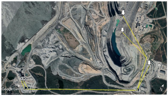
Figure 1.
Overview of the southeast part of the mine, with the crushers, stockpiles, and the mills marked with white arrows, triangles, and circles, respectively. The yellow line shows the approximate trace of the conveyors. Created with Google Earth Pro.
2. Materials and Methods
The methodology of the study is presented on Figure 2. A lack of knowledge was identified regarding the transportation time between the mine face and the mill in the ongoing mine-to-mill study in Aitik. A literature study was carried out on previous mine-to-mill and ore transportation research. Then, the virtual silo approach was selected for the current study, which uses historical production data. The Aitik mine’s ore transportation system between the production face and the mills is described at the end of Section 1. The transportation system was modeled as a virtual silo [12,13] with input data from the truck dispatch and the mineral processing control and monitoring system logs. Data was provided by Boliden Minerals AB, from the ABB and Minestar Data Archives of the Aitik mine.

Figure 2.
Process map of the study.
The average transportation time is calculated based on the most common tonnage and ore levels; then, the mass balance is calculated with both the cumulative and the momentary outflow. The results are compared to each other, and with the mean transportation time based on the mean values of the ore mass in the virtual silo and the outflow.
3. Results
3.1. Calculating Transportation Time in a Virtual Silo by Back Propagation and Prognosis
First, two means of transport time calculations are presented for a general virtual silo. A general form of the virtual silo with k time-dependent mass inflows and l time-dependent mass outflows is presented in Figure 3. At this point, the inner complexity of the silo is not considered, and the mstored(t) time-dependent mass stored in the silo is used.
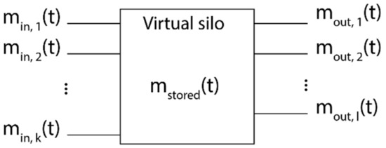
Figure 3.
General form of a virtual silo with k inflows and l outflows. Redrawn after [13].
If only one type of material is transported, the in- and outflows can be simplified to a sum of the inflows and the sum of the outflows. Equation (1) presents the sum of all the inflows at time t.
Equation (2) presents the sum of all outflows at time t.
In order to calculate the transportation time in a first in-first out model where the material does not blend, two means are used: calculation by back propagation, or mass balance accounting; and prediction at time t′.
The mass balance accounting is undertaken as follows: the cumulative mass inflow and the cumulative mass outflow are calculated, and the cumulative flows are marked by M(t).
The mass is calculated at the outflow, after the silo, so the cumulative mass inflow at time t is the sum of the stored mass at t0, the beginning of the time series, and the summed mass inflow from t0 until t, as shown in Equation (3). The cumulative mass outflow is calculated as the sum of the outflow from t0 until t, as shown in Equation (4).
The transportation time at time t in this case is calculated as the minimum Δt, subject to:
Equation (5) represents the queueing in the transportation, where the transportation time Δt is the time it takes for the cumulative outflow to reach the same value as the cumulative inflow at a specific time t.
The predicted time Δt is calculated by dividing the mass stored in the virtual silo by the momentary outflow value, as shown by Equation (6).
The difference between the two types of calculations is graphically presented in Figure 4. As shown, even when mstored(t) is known accurately, the predicted and the back-tracked times may differ due to variations in the outflow.
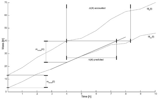
Figure 4.
Graphical representation of the cumulative mass inflow Min(t) (dashed) and cumulative mass outflow Mout(t) (dotted). The transportation time is calculated at time 4. The horizontal distance of Min(4) and Mout(t) represents the back-calculated time. The predicted time is the horizontal distance between the Min(4) and the solid black tangential line at Mout(4).
3.2. Boliden Aitik Ore Transportation System
Figure 5 shows the ore transportation process layout from the crushers to the primary mills. The intermediate stockpile is a hall with two inflows from the surface and the in-pit crushers, dumping the crushed rock from the top. Five belt feeders draw the piled ore from the bottom and feed a conveyor belt that transports the ore to one of the two main stockpiles. The main stockpiles are similar to the intermediate stockpile, but each with almost triple the capacity of the intermediate stockpile.
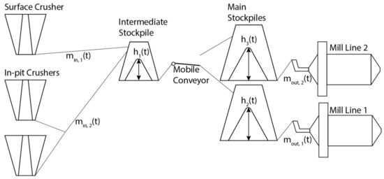
Figure 5.
Layout of the ore transportation system between the crushers and the primary mills.
The stockpiles are loaded one at a time, with a mobile conveyor belt used to switch between them. The mill lines consist of the conveyors from the stockpiles to the autogenous primary mills, continued by secondary pebble mills and a pebble crusher. The comminution circuits feed the flotation circuit where the ore minerals are separated from the tailings.
A scale is installed after each crusher and after each stockpile. The scales after the main stockpiles are calibrated by a third-party company at regular intervals [24]. The other scales on the conveyor line are calibrated on demand by company technicians [24]. The measurement of the scales after the main stockpiles are used to account for the throughput, so they are accepted as accurate [24]. The tonnages of the other belts have to be checked if there is an offset in their measurement.
To control the outflow below, each feeder to the belt conveyor is equipped with a radar that measures the ore level above the feeder; if the ore level above a feeder is too low, the feeder stops [24]. This is to prevent damage to the feeder from the ore falling from the top. If the ore level is too high in a stockpile, the feeder of the previous station is stopped to prevent overflow [24]. The ore beneficiation process is operated and monitored through the ABB800 XA system, which records all data continuously. The ore level measurements are used as an approximation of the ore stored in the stockpiles. h1, h2, and h3 represent the mean of the ore level measurements in the intermediate stockpile, main stockpile 1, and main stockpile 2, respectively.
Momentary records are saved every 6 s and stored for a week. Averages by the minute are calculated and stored for one year. In this study, per-minute conveyor belt tonnages and per-minute ore level measurements are used from the ABB system. As inputs to the circuit, the truck dumping time and payload records are used from the Fleet Management System. According to local practices, the intermediate stockpile is managed differently during freezing and non-freezing conditions. Due to this, the model was developed and tested on data from two months: February (when temperature was below zero Celsius) and June (when it was above).
3.3. Virtual Silo Model Development for the Aitik Transportation Line
Since the transportation times on the conveyor belt are very similar for the in- and the outflows, one inflow and one outflow is defined for the virtual silo. The virtual silo is modeled as the collection of the three stockpiles without internal flow. Figure 6 presents the inflow, outflow, and mass storage components of the virtual silo.
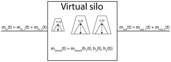
Figure 6.
The defined virtual silo with a time-dependent mass inflow, mass outflow, and stored mass dependent on the time-dependent ore heights in the stockpiles.
The virtual silo model is developed in three stages:
- Based on the available ore level and conveyor belt tonnage data, the accuracy of the tonnage data is checked by comparing the cumulated net mass flow in the stockpiles against the median ore level.
- The ore level–ore mass relationship is established for each stockpile in the system for the months of February and June.
- Based on the now available system parameters, the virtual silo is outlined and a mathematical formula is given for the mass stored in it based on the momentary average ore levels in each stockpile.
3.3.1. Scale Accuracy
During the examination of the scale accuracy, the variations in the ore quality are not considered. This is done for two reasons. First, the main ore types are schists and gneisses, which have identical densities [22]; second, there is a huge uncertainty in the actual ore quality in the transportation system at a given time. This uncertainty can be addressed after the basic transportation model is established; therefore, it is out of the scope of the current study.
As mentioned in the ore transportation system site description, the scales after the main stockpiles are regularly calibrated by a third-party company and, as such, they are accepted as accurate. However, the accuracy of the scale of the conveyor connecting the intermediate stockpile to the main stockpiles has to be checked. The possible offset of the conveyor connecting the intermediate and the main stockpiles is measured as follows: the median ore level in meters is selected for the main stockpiles throughout both tested periods. The net flow in the stockpile (inflow-outflow) is summed during the tested periods, as shown in Figure 7. Assuming that the same ore level represents the same ore mass in the stockpile with good accuracy, the mass balance can be assumed to be constant at any arbitrarily selected ore level in the tested periods.
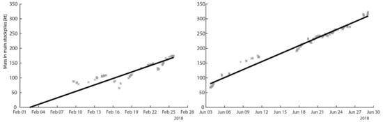
Figure 7.
Cumulative ore mass of the two main stockpiles at the median ore level based on the measured net ore flow. The accumulation of ore at a constant level means that more inflow is measured than outflow, which indicates inaccuracy at the scales.
As seen in Figure 7, the net mass in the stockpile increases at the same ore level, which means that more inflow is measured than outflow. Since the outflow measurement is accepted as accurate, this result means that the inflow tonnage measurement is not accurate and more tonnage is registered than the flow-through in reality. Linear regression shows the offset of the conveyor connecting the intermediate and main stockpiles. The slope of the baseline shift is 304.4 t/h in February and 375.7 t/h in June. The designed capacity of the conveyor belt between the intermediate stockpile and the main stockpile is 7 kt/h. This means that the difference in the baseline shift is approximately +4.4% in February and +5.4% in June. The positive value means that the measurement shows higher tonnage than the actual value.
In the following calculations, this estimated correction factor is subtracted from the tonnages of the intermediate stockpile conveyor belt. The conveyor belts after the crushers were not used in this study; instead, the truck payloads were used for the inflow. The total payloads during the examined months were within a difference of 1% compared to the total outflow, not considering the differences in the ore level measurements in the stockpiles. Because of this, the truck payloads are accepted as accurate measurements.
3.3.2. Establishing Ore Level-Ore Mass Relation
For each stockpile, the ore level change in a selected time period is compared with the net mass flow. Since the intermediate stockpile is loaded directly from the crushers, which provide fluctuating inflow, the ore mass change per meter is calculated as follows. Each time section when the inflow is less than 150 tonnes per h was selected with their timestamp and duration. Six scenarios were examined ranging from 5 to 30 min. The different scenarios were selected to check for possible differences in characteristics in short- and long-term decrease. For each section, linear regression was used and the increment of the line was divided by the output tonnage. This yields a coefficient that has a unit of meters per kiloton, which shows how much the mean ore level increases by removing one kiloton ore of from the stockpile.
The determined coefficients for each stockpile in each month and for each minimum duration were statistically tested against each other as follows:
- Two-tailed t-tests for each minimum duration for the intermediate stockpile February and June coefficients
- One-way analysis of variance (ANOVA) for the different minimum durations for both the February and June coefficients in the intermediate stockpile
- One-way ANOVA for each minimum duration for the main stockpiles 1 and 2 coefficients in February and June
The t-test results showed that the February and June coefficients were significantly different for each minimum duration for the intermediate stockpile, with the coefficients in February being 20% higher than in June. This observation is in line with the notation of different operational practices for the intermediate stockpile during winter and summertime, namely, that at cold temperatures the operators aim to keep the ore fill low in the intermediate stockpiles to avoid the freezing of the ore, which could result in problems in the downstream transportation. Analysis of variance (ANOVA) showed that the coefficients were statistically not significantly different for different minimum durations starting from a minimum of 10 min, both for the February and June coefficients of the intermediate stockpile, meaning that the rate of decrease in the intermediate stockpile is similar at shorter and longer durations with constant outflow, except when the outflow time is shorter than 10 min. Figure 8 presents the results of the ANOVA for the intermediate stockpile.
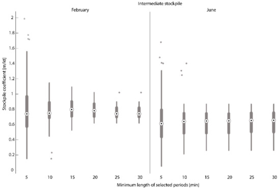
Figure 8.
Box plot of the coefficients for different minimum durations in February and June for the intermediate stockpile.
In the case of the main stockpiles, the ANOVA showed that at a 5% significance level, starting at a minimum duration of 25 min, the coefficients are not significantly different for the main stockpiles 1 and 2, regardless of whether it is February or June. The distribution of coefficients for the main stockpiles is presented in Figure 9. It should be noted that the y-scale on Figure 9 ranges from 0 to 1 m/kt, whereas the same y-axis on Figure 8 ranges from 0 to 2 m/kt. The scales were selected to better represent the majority of the stockpile coefficients. The interquartile range of the intermediate stockpiles has a similar length, of between 0.2–0.3 m/kt in all cases.
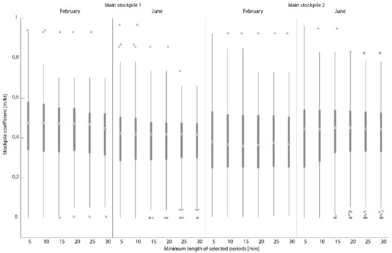
Figure 9.
Analysis of variance of the main stockpile coefficients for the different minimum durations.
The results show that the same coefficient is appropriate to use in the main stockpiles in both the February and June data, for both main stockpiles. The results also show that the coefficients are from the same population with high probability for different minimum durations, which indicates that the ore mass in the storage has a linear relationship with the mean ore level in each stockpile. Table 1 presents the mean and maximum of the coefficients and the number of sections for the intermediate stockpile in February and June, and all the sections combined for the main stockpiles. The number of sections decreases radically with a longer minimum length for the intermediate stockpile

Table 1.
Mean coefficients and number of separate unloading events at the intermediate February stockpile, the intermediate June stockpile, and the main stockpiles.
The coefficients are calculated at this step, and thus the ore mass in each stockpile is calculated as shown in Equation (7).
where:
- mi is the ore mass
- hi is the average of the five ore level measurements, and
- ci is the previously defined coefficient or slope
of the i-th stockpile, where i = 1 is the intermediate stockpile, i = 2 is the main stockpile 1, and i = 3 is the main stockpile 2. The ore mass in the virtual silo is calculated as the sum of the ore masses in the stockpiles, as shown in Equation (8).
3.4. Transportation Time Calculations
After establishing the virtual silo model, it was tested on the available ore level, tonnage, and truck dispatch data. Three different scenarios were considered:
- Average transportation time based on the available ore level and tonnage data.
- Transportation time accounting as was introduced with the virtual silo, based on the detailed mass-flow logs based on the dispatch data (min) and the combined tonnages at the mills (mout).
- Predicted transportation time based on the ore mass calculation at the moment of each truck unloading, and the momentary outflow values.
The average transportation time is calculated as follows. The calculated ore mass in the virtual silo is rounded to 1000 tons, and the mode is selected. Then, the tonnage of the two conveyor belts is rounded to 100 t/h, and the mode is selected. The mode ore mass is divided by the mode outflow, resulting in the transportation time for the most frequent outflow and ore mass values. This results in 16.5 h for February and 18.5 h in June.
The accounted transportation time is calculated as follows. The transportation mode is assumed to be first in-first out; the truckloads are queued after each other. The ore mass in the virtual silo is calculated at the beginning of the time period, and each truckload is queued such that the payload of the trucks is summed and added to the ore mass in the virtual silo, as shown in Equation (9). Each truckload receives an increasing payload value, and trucks dumping at a later time have a higher payload number.
Equation (10) shows how the outflow tonnages are summed, similarly to the inflow. The transportation time is calculated as the duration of time between the truck payload timestamp and the timestamp of the lowest outflow tonnage that is larger than the payload tonnage, as defined in Section 3.1 in Equation (5).
The predicted transportation time at time t is calculated by dividing the ore mass at t by the outflow at t, as shown in Equation (11).
Figure 10 displays the time series of the calculated ore mass and the outflow in the virtual silo, and the calculated transportation times. Figure 10a shows that the ore level-based calculation underestimates the ore mass in the virtual silo compared to the mass balance-based calculation. The mass balance-based line starts with a lag; this is due to the mass balance calculated after the first truck dump in the month, and there was no feed arriving from the mine in the first day of the month. Figure 10b,c show that the predicted times are directly related to the outflow. When outflow drops to near zero, the predicted transportation time increases drastically. Approximately 1% of all the predicted transportation times in February exceeded 100 h, due to occasional drops in the outflow. These values were filtered out. The best example is after 7 February, when the outflow drops to zero for 6 h. This can be explained by a planned or emergency maintenance stop.
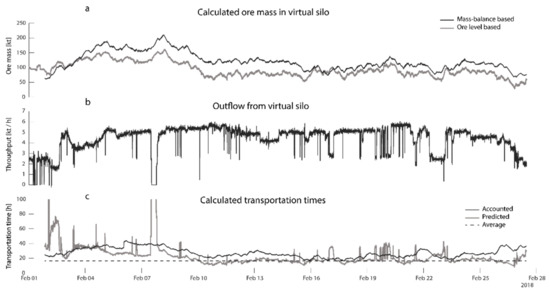
Figure 10.
Subfigure (a) shows the calculated ore mass based on the mass-balance (black) and the ore levels (grey). Subfigure (b) shows the outflow. Subfigure (c) shows the average (dashed), the accounted (black) and the predicted (grey) transportation times in February.
Figure 11 presents the distribution of the transportation times in February. The dashed line presents the calculated average, the grey histogram is the distribution of the predicted values, and the patterned line distribution represents the accounted values. The most frequent predicted times and the average time coincide. This is expected, as the average time was calculated based on the mode, the most frequent values of the ore mass in the virtual silo, and the outflow. The most frequent predicted value is between 16 and 17 h, the majority of the predicted transportation times are between 12 and 20 h, and 57% of the times are between 16 and 20 h. The most frequent accounted value is between 24 and 25 h, and 52% of the accounted values are between 18 and 26 h.
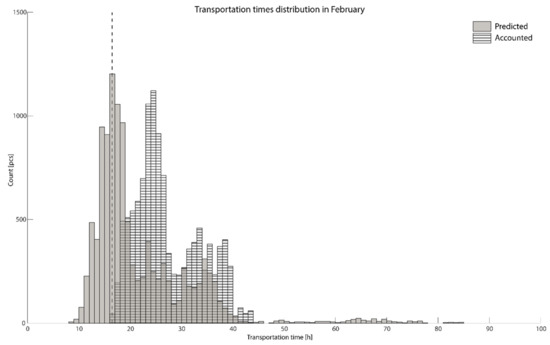
Figure 11.
Distribution of the transportation times. The dashed line is the calculated average, grey represents the predicted times, and striped represents the accounted transportation times in February.
Both the predicted and the accounted values have two minor peaks, at 24 and 35 h, and 34 and 39 h, respectively. The distributions show a skewness to the left. This can be explained by the stockpile management: the amount of the ore in the system cannot go too low, because then the feeders cannot operate due to safety reasons. In addition, because there is a risk at low stock that the mills have to be shut down due to the lack of feed, too low stock is avoided. Overfilling was not experienced during the tested time.
Figure 12 shows the calculated ore mass (a) and the outflow (b) in the virtual silo, and the calculated transportation times (c). Figure 12a shows an increasing trend for the mass balance-based calculation. The reason for this may be an additional offset in the scales, which was not considered in the previous calculations. This may originate from the trucks’ side, or from the scales before the mill, even though the calculations accepted them as accurate. A sudden increase can be seen in Figure 12a at the end of June. At the same time, the outflow drops to half the value, which could be seen throughout the month. The drop in the outflow on Figure 12b, combined with the increased quantity of ore in the virtual silo, hints at a planned maintenance stop. There are also short-term drops throughout the month on Figure 12b; these can be explained by short stops of one of the conveyor lines. The reasons for these short stops are not clear.
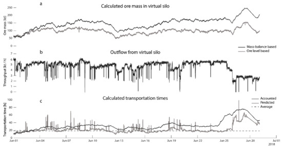
Figure 12.
Subfigure (a) shows the calculated ore mass based on the mass-balance (black) and the ore levels (grey). Subfigure (b) shows the outflow. Subfigure (c) shows the average (dashed), the accounted (black) and the predicted (grey) transportation times in June.
Figure 12c shows that the ore level-based calculation underestimates the ore mass in the virtual silo compared to the mass balance-based calculation. An increasing trend can be seen in the mass balance-based calculation. This may be due to inaccuracy in the scales of the trucks or in the transportation line.
In the bottom graph, the predicted times are directly related to the outflow; when outflow drops to near zero, the predicted transportation time increases drastically. Approximately 0.25% of all the predicted transportation times in June exceeded 100 h, due to occasional drops in the outflow. These values were filtered out. It should be noted that the accounted and predicted transportation times do not show as much difference as the mass balance- and ore level-based ore mass.
Figure 13 shows the distribution of the transportation times in June. The dashed line presents the calculated average, the grey histogram is the distribution of the predicted values, and the patterned line distribution presents the accounted values. The most frequent predicted times and the average time coincide. This is expected, as the average time was calculated based on the mode, the most frequent values of the ore mass in the virtual silo, and the outflow. The most frequent predicted value is between 18 and 19 h, and 68% of the predicted transportation times are between 16 and 24 h. The most frequent accounted values are between 30 and 31 h and 52% of the accounted transportation times are between 26 and 34 h.
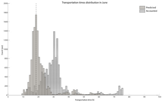
Figure 13.
Distribution of the transportation times. The dashed line is the calculated average, grey represents the predicted times, and striped represents the accounted transportation times in June.
In the June dataset, the accounted and predicted times differ more than in the February dataset. Two explanations arise. One is related to the remnant baseline shifting in the ore mass in the system that was shown on the top graph in Figure 12. As the mass balance indicated increasingly more mass in the silo than calculated by the ore level measurements, the increasing difference in mass resulted in an increased transportation time. The second reason is that at the end of June, a significant rise can be observed in the ore mass in the system, and a sudden drop in the outflow at the same time. This behavior is due to a maintenance stop in one of the mill lines. The grinding capacity halves, but is not compensated for at the time by the lower quantity of ore being fed to the crushers from the mine, resulting in mass accumulation in the system. Because it is backwards calculated, the accounted times start to increase even before the maintenance stop happens, increasing the difference between the two types of calculations.
4. Discussion
In this study, the authors presented two methods to calculate transportation time between the crusher and the mill. One of the calculations was based on mass balance between the in- and outflows in the transportation system. This was modeled as one virtual silo, containing the summed ore mass of the stockpiles in the system where the flow type was set as first in-first out. The other calculation was based on the momentary outflow and the mass in the stockpile, calculated using the momentary ore level measurements.
Based on the data from the two test periods, the following conclusions can be made for the transportation model:
- As was shown in the ore level vs. ore mass calculations in the presented case, the average ore level measured above the feeders in the stockpiles’ operational height range changes linearly with the mass decrease caused by a constant outflow rate.
- All calculated transportation time distributions are skewed to the left. This can be explained by stockpile management practices, namely, that the ore mass stored in the transportation system should be large enough to provide feed for the mill for a certain time in case of disruption at the mine. It is possible to stock more ore in the transportation systems, but keeping significantly more ore in the stockpile for an extended time is not necessary because it does not happen often.
- The predicted times have a larger skew than the accounted times. This is explained by the direct dependency on the momentary outflow of the predicted values. At low outflows, the predicted values significantly exceed the accounted ones.
- The predicted transportation times are generally several hours lower than the accounted ones, as was shown on Figure 10 and Figure 12. The key explanation for this is that the outflow is rarely operated at a constant level for long times, e.g., 24 h or more. The outflow can be decreased due to various reasons in the milling operation, e.g., because of feeding harder ore to the mill that takes more time to grind, or because of low ore levels in the system, when the outflow has to be decreased to avoid shutting down due to a lack of feed.
- The largest differences between the queuing and momentary outflow-based calculations were found in the beginning of February and at the end of June. These were connected to longer disturbances in the outflow, which can be explained in terms of stopping one of the two outflow lines in the physical system, e.g., for maintenance purposes. In Figure 10, in the beginning of the month, the outflow fluctuates between zero and half of the outflow during most of the month. In Figure 12, a large accumulation of ore mass can be seen at the end of the month, which implies a mine-scale maintenance stop. If decisions are made regarding production during times when one mill line does not work, the transport times are underestimated badly if momentary values are used.
5. Future Work
The presented virtual silo model will be upgraded by adding internal flow to the virtual stockpile, and treating the two physical output lines as two virtual outputs instead of one. This will enable separate evaluation of the mill feed on the two mill lines.
The first in-first out flow will be replaced with mass and funnel flow states. Mass flow is similar to first in-first out flow, but a mixing effect should be considered in the stockpiles; in funnel flow, a large part of the stockpile becomes stagnant, which results in a significantly reduced active zone and transportation time.
Author Contributions
Conceptualization, B.V. and D.J.; methodology, B.V.; software, B.V.; formal analysis, B.V.; investigation, B.V.; resources, D.J.; data curation, B.V.; writing—original draft preparation, B.V.; writing—review and editing, B.V., D.J. and H.S.; visualization, B.V.; supervision, D.J. and H.S.; project administration, D.J.; funding acquisition, D.J. All authors have read and agreed to the published version of the manuscript.
Funding
This research was funded by Vinnova, the Swedish Energy Agency and Formas through 3rd party data.
Data Availability Statement
Data was obtained from Boliden Aitik Mine, and are available from the authors with the permission of Boliden Aitik Mine.
Acknowledgments
The authors acknowledge Boliden Minerals AB and the staff and management of the Boliden Aitik Mine for valuable input and support during field studies and data access. The authors would like to acknowledge the support from Center for Advanced Mining and Metallurgy (CAMM2), Sweden.
Conflicts of Interest
The funders had no role in the design of the study; in the collection, analyses, or interpretation of data; in the writing of the manuscript, or in the decision to publish the results.
References
- McKee, D.J.; Chitombo, G.P.; Morrell, S. The relationship between fragmentation in mining and comminution circuit throughput. Miner. Eng. 1995, 8, 1265–1274. [Google Scholar] [CrossRef]
- Bergman, P. Optimisation of fragmentation and comminution at Boliden Mineral, Aitik Operation. Licentiate Thesis, Luleå University of Technology, Luleå, Sweden, 2005. [Google Scholar]
- Wambeke, T.; Elder, D.; Miller, A.; Benndorf, J.; Peattie, R. Real-time reconciliation of a geometallurgical model based on ball mill performance measurements—A pilot study at the Tropicana gold mine. Min. Technol. 2018, 127, 115–130. [Google Scholar] [CrossRef] [Green Version]
- Nadolski, S.; O‘Hara, C.; Klein, B.; Elmo, D.; Hart, C.J.R. Cave fragmentation in a cave-to-mill context at the New Afton mine Part II: Implications to mill performance. Min. Technol. 2018, 127, 155–166. [Google Scholar] [CrossRef]
- Nageshwaraniyer, S.S.; Kim, K.; Son, Y.-J. A mine-to-mill economic analysis model and spectral imaging-based tracking system for a copper mine. J. S. Afr. Inst. Min. Metall. 2018, 118, 7–14. [Google Scholar] [CrossRef]
- Valery, W.; Dance, A.; Jankovic, A.; Larosa, D.; Esen, S. Process integration and optimization from mine-to-mill. In Proceedings of the International Seminar on Mineral Processing Technology, Mumbai, India, 22–24 February 2007; Khosla, N.K., Jadhav, G.N., Eds.; Allied Publishers Pvt. Ltd.: Mumbai, India, 2007; pp. 577–581. [Google Scholar]
- Meech, J.A.; Baiden, G.R. Simulating the mine-mill interface. Int. J. Surf. Mining Reclam. Environ. 1987, 1, 191–198. [Google Scholar] [CrossRef]
- Servin, M.; Vesterlund, F.; Wallin, E. Digital twins with distributed particle simulation for mine-to-mill material tracking. Minerals 2021, 11, 524. [Google Scholar] [CrossRef]
- Metso:Outotec: Ore Tracking. Available online: https://www.mogroup.com/products-and-services/services/process-optimization-connected-services/ore-tracking/ (accessed on 11 November 2021).
- Jansen, W.; Morrison, R.; Wortley, M.; Rivett, T. Tracer-Based Mine-Mill Ore Tracking via Process Hold-ups at Northparkes Mine. In Proceedings of the Tenth Mill Operators’ Conference, Adelaide, Australia, 12–14 October 2009; The Australasian Institute of Mining and Metallurgy (The AusIMM): Adelaide, Australia, 2009; pp. 345–356. [Google Scholar]
- Kvarnström, B.; Nordqvist, S. Modelling process flows in continuous processes with radio frequency identification technique. In Proceedings of the International Conference on Process Development in Iron and Steelmaking, Lulea, Sweden, 8–11 June 2008; MEFOS: Lulea, Sweden, 2008; pp. 253–262. [Google Scholar]
- Itävuo, P.; Väyrynen, T.; Vilkko, M.; Jaatinen, A. Tight feed-hopper level control in cone crushers. In Proceedings of the IMPC 2014—27th International Mineral Processing Congress, Santiago, Chile, 20–24 October 2014; IMPC: Santiago, Chile, 2014. [Google Scholar]
- Itävuo, P.; Hulthén, E.; Yahyaei, M.; Vilkko, M. Mass balance control of crushing circuits. Miner. Eng. 2019, 135, 37–47. [Google Scholar] [CrossRef]
- Panday, R.; Breault, R.; Shadle, L.J. Dynamic modeling of the circulating fluidized bed riser. Powder Technol. 2016, 291, 522–535. [Google Scholar] [CrossRef] [Green Version]
- Blaszczuk, A.; Zylka, A.; Leszczynski, J. Simulation of mass balance behavior in a large-scale circulating fluidized bed reactor. Particuology 2016, 25, 51–58. [Google Scholar] [CrossRef]
- Ajayi, O.O.; Sheehan, M.E. Pseudophysical Compartment Modeling of an Industrial Rotary Dryer with Flighted and Unflighted Sections: Solids Transport. Ind. Eng. Chem. Res. 2014, 53, 15980–15989. [Google Scholar] [CrossRef]
- Jenike, A.W. Storage and Flow of Solids: Bulletin No. 123; University of Utah: Salt Lake City, UT, USA, 1964; Volume 53. [Google Scholar]
- Nguyen, T.V.; Brennen, C.E.; Sabersky, R.H. Funnel Flow in Hoppers. J. Appl. Mech. 1980, 47, 729–735. [Google Scholar] [CrossRef]
- Magalhães, F.G.R.; Atman, A.P.F.; Moreira, J.G.; Herrmann, H.J. Analysis of the velocity field of granular hopper flow. Granular. Matter 2016, 18, 33. [Google Scholar] [CrossRef] [Green Version]
- Boliden. Metals for Future Generations: Boliden Annual and Sustainability Report 2020; Boliden: Stockholm, Sweden, 2021. [Google Scholar]
- Knipfer, S.; Nordin, R.; Wasström, A.; Höglund, S.; Joslin, G.; Wanhainen, C. The Aitik porphyry Cu-Au-Ag-(Mo) deposit in Sweden. In Proceedings of the 11th SGA Biennial Meeting “Let’s Talk Ore Deposits”, Antofagasta, Chile, 26–29 September 2011; pp. 1–3. Available online: http://ltu.diva-portal.org/smash/record.jsf?pid=diva2:1012613 (accessed on 15 January 2022).
- Beyglou, A. Target fragmentation for efficient loading and crushing—The Aitik case. J. South. Afr. Inst. Min. Metall. 2017, 117, 1053–1062. [Google Scholar] [CrossRef] [Green Version]
- Beyglou, A.; Schunnesson, H.; Johansson, D. Face to Surface—Task 1: Baseline Mapping of the Mining Operation in Aitik; Research Report; Luleå University of Technology: Lulea, Sweden, 2015; p. 79. [Google Scholar]
- Thomas, S.; Boliden Mineral AB, Stockholm, Sweden. Personal communication, 2019.
Publisher’s Note: MDPI stays neutral with regard to jurisdictional claims in published maps and institutional affiliations. |
© 2022 by the authors. Licensee MDPI, Basel, Switzerland. This article is an open access article distributed under the terms and conditions of the Creative Commons Attribution (CC BY) license (https://creativecommons.org/licenses/by/4.0/).