Grey Box Modelling of Decanter Centrifuges by Coupling a Numerical Process Model with a Neural Network

Abstract

Continuously operating decanter centrifuges are often applied for solid-liquid separation in the chemical and mining industries. Simulation tools can assist in the configuration and optimisation of separation processes by, e.g., controlling the quality characteristics of the product. Increasing computation power has led to a renewed interest in hybrid models (subsequently named grey box model), which combine parametric and non-paramteric models. In this article, a grey box model for the simulation of the mechanical dewatering of a finely dispersed product in decanter centrifuges is discussed. Here, the grey box model consists of a mechanistic model (as white box model) presented in a previous research article and a neural network (as black box model). Experimentally determined data is used to train the neural network in the area of application. The mechanistic approach considers the settling behaviour, the sediment consolidation, and the sediment transport. In conclusion, the settings of the neural network and the results of the grey box model and white box model are compared and discussed. Now, the overall grey box model is able to increase the accuracy of the simulation and physical effects that are not modelled yet are integrated by training of a neural network using experimental data.

1. Introduction

Decanter centrifuges are continuously working apparatuses for solid-liquid separation [1]. Within the centrifuge, settling, sediment consolidation, and sediment transport take place simultaneously. The machine is flexible in its application through a variety of adjustable machine and process variables. These parameters, however, influence each other, so that the same separation result can be obtained with different combinations of parameters [2]. This increases the difficulty of dimensioning and modelling the decanter centrifuge. There are three general modelling options: purely parametric modelling, purely non-parametric modelling, or a combination of both.

The use of artificial neural networks (ANN) as non-parametric models to solve engineering tasks has increased in the recent years [3,4,5,6]. These networks serve as universal function approximators, i.e., they are able to reflect arbitrarily defined model functions. The advantage of an ANN-based model is that it can be created and used without an a-priori knowledge of the physical correlations in the actual process. But, the setup of an ANN requires knowledge and experience about how to create such a model. However, the quality and quantity of the data available for training and testing are crucial. If the data is noisy or sparse, the reliability of the ANN decreases. On the other hand, relevant parameters are often available and mathematical-physical basic equations, empirical correlations, or numerical models already exist as parametric models investigating technical processes. However, such approaches are often connected with specific assumptions, which, in some cases, can deviate significantly from reality. Grey box modelling represents a modelling approach that consists of a parametric and a non-parametric model. Combining the two principal methods has several advantages compared to the individual view, which is described more detailed later in this article.

Gonzalez-Fernandez et al. [7] provide a review of publications about the use of artificial intelligence in olive oil production, where centrifuges are commonly used.

Funes et al. [8] introduce an ANN predicting quality parameters of olive oil during its processing in a disc stack separator. Process variables, like the feed temperature and the feed flow of oil must and water and the temperature and the flow of oil at the outlet, serve as input parameters for the ANN. Near-infrared sensors at the outlet measure specific quality parameters, which are used as output parameters. The feed-forward, backpropagation ANN is designed to correlate the quality parameters as a function of the process variables to predict the machine and product behaviour for process regulation and optimisation.

Jiménez et al. [9,10] use a neural network designed for the optimisation of an olive oil elaboration process in a decanter centrifuge. Qualitative parameters of the fruit, like fat content and moisture, and process variables of the feed, like temperature, flow rate, and dilution ratio serve as input. The aim is to predict the fat content of olive pomace and oil moisture by means of applying an ANN. The authors have shown that this approach allows reasonable predictions for this specific application. However, the authors also clarify that the influence of other essential process variables of the machine, such as pool depth, rotational speed, and differential speed, cannot be predicted with the neural network based on the applied training data set. This requires either an extension of the training data regarding the effects to be modelled or mathematical models that describe the correlations.

In general, purely ANN modelling approaches are often highly specialised for their purpose. Thus, transfer to other applications or extension of variables, if it is necessary, require redesign and further training of the system. The generalisation of such approaches is often a major challenge.

Thompson and Kramer [11] present a method to develop a grey box model in chemical processes. They use a simple process model, boundary conditions and equations known beforehand to enhance a neural network. This supports the network to compensate for the lack and low quality of the data, and thus extends the range of application. As an exemplary case study, the authors describe the synthesis of a grey box model for a fed-batch penicillin fermentation.

Menesklou et al. [12] introduce a dynamic process model for decanter centrifuges. The model enhances the work by Gleiss et al. [13] integrating the conical part of the decanter centrifuge. Furthermore, improved material functions are derived to consider shear thickening effects during sediment consolidation. This mechanistic approach considers settling behaviour, sediment consolidation and sediment transport. Additionally, the authors have validated the model with experiments using different calcium carbonate water slurries and decanter centrifuges from lab- to industrial-scale [14]. In some applications, for example at relatively deep pool depths, local turbulence and flows in some areas of the centrifuge can influence the separation result. The assumption of a plug flow in these areas is no longer applicable. One possibility to characterise this behaviour is a complex flow simulation using Computational Fluid Dynamics (CFD) [15]. An alternative possibility is the use of a grey box model. The articles described previously have shown that it is indeed possible to model technical processes and especially centrifuges using ANN. However, these cases are often very specific and typically limited to their specific applications. Combining a numerical process model, for example as described in Menesklou et al. [12], with a neural network is intended to extend and generalise the overall range of applications.

This article presents the development of a grey box model based on a dynamic process model and a neural network. For this purpose, the parametric model by Menesklou et al. [12] is combined with a neural network and trained with experimental data to consider such specific flow effects on the separation behaviour at rather deep pool depths. In general, this extends the application range of the numerical process model without losing the advantages of a process model. As a result, the simulation tool can learn to consider further effects and thus to increase its accuracy and scope.

2. Theory

This section provides an overview of the theoretical background of grey box modelling and neural networks, which are both used in this article.

2.1. Grey Box Modelling

White box, black box, and grey box models represent three different modelling strategies. The white box model is purely theoretical and parametric. This means that, based on known mathematical and physical correlations and principles, the required variables can be obtained. These correlations range from simple analytical equations and existing empirical correlations to complex differential equations and simulation approaches, which require numerical methods to be solved. Although the process behaviour may be difficult to model, the calculations are fully comprehensible. Therefore, the white box model is often called glass box model or clear box model because a view into the equations is possible. In contrast, there is the so-called black box model, which provides output parameters for specific input parameters. The black box model does not use common equations with physical background to obtain the output parameters. It relates output and input data to obtain empirical correlations, which were not understood previously.

The grey box model is a combination of the two previously mentioned models. Principally, they can be arranged in series or parallel in the internal structure. For example, Psichogias and Ungar [16] used a serial structure for model based control and process modelling of fermentation. Furthermore, Pitarch et al. [17] used a more interconnected grey box modelling approach with submodels, which integrate regression equations among internal variables into first principles ones. Figure 1 illustrates a parallel grey box model structure, which is used in the present work.

The input variables are defined in the vector ${\overrightarrow{x}}_{\mathrm{in}}$, which is transferred to the white box and black box model. On the one hand, the parametric model serves as an ideal approximator for the considered process output variables ${\overrightarrow{y}}_{\mathrm{id}}$, which contains all required assumptions and simplifications. On the other hand, the non-parametric model is adjusted to determine deviations between the ideal model and actual available data and gives the output ${\overrightarrow{y}}_{\mathrm{cor}}$. Both (${\overrightarrow{y}}_{\mathrm{id}}$ and ${\overrightarrow{y}}_{\mathrm{cor}}$) are combined by a function $f_{\mathrm{com}}$ that returns the total output value of the grey box model. The function is selected according to the objective of the black box model. For example, it can be a simple addition or subtraction. By systematically calibrating the non-parametric model, the resulting grey box model is able to consider the physical behaviour, which is not included in the parametric model yet.

2.2. Artificial Neural Networks

Artificial neural networks are computational and mathematical model systems whose structure is reminiscent of the network of neurons in the neuronal system of living beings. In general, they consist of neurons, weighted connections, and activation functions, which are grouped in layers. Neurons receive multiple input signals from other neurons and send one output signal to multiple other neurons. Tendentially, the more neurons a layer of a neural network has, the more complex issues it can handle. Each connection between neurons is weighted according to its importance. This is the key feature because prioritising connections leads to the ability of learning. The activation function calculates the output of a neuron as a function of its input. Additionally, a bias vector can be added. Figure 2 depicts exemplarily a neural network with one hidden layer.

The vector ${\overrightarrow{x}}_{\mathrm{in}}$ with M predefined parameters forms the input layer. Each parameter transmits a signal to the $N_{\mathrm{n}}$ neurons in the hidden layer. The weighted input signals are summarised with a bias vector $\overrightarrow{b}$,

$$\overrightarrow{n}=W{\overrightarrow{x}}_{\mathrm{in}}+\overrightarrow{b},$$

(1)

which is the argument for the activation function f. The weight matrix,

$$W=\left(\begin{array}{cccc}{w}_{1,1}& w_{1,2}& \cdots & w_{1,M}\\ w_{2,1}& w_{2,2}& \cdots & w_{2,M}\\ ⋮& ⋮& \ddots & ⋮\\ w_{N_{\mathrm{n}},1}& w_{N_{\mathrm{n}},2}& \cdots & w_{N_{\mathrm{n}},M}\end{array}\right),$$

(2)

contains all single weights. The bias vector is an additional, special neuron for each layer. It stores a scalar value, typically one. This is necessary to make the output of the activation function more flexible. The neural network in this article uses supervised learning. This type learns with training data, consisting of paired values, such as experimental data measured under specific conditions. Training success is evaluated and used to improve the accuracy of the neural network. The quality of the algorithm is examined using test data. Backpropagation is one training strategy of supervised learning. The output of the neural network is compared to the correct answer of the training data to determine the error function. This error is fed back through the network to adjust the weights. The process is repeated until the error is sufficiently small. Generally, the information within the neural network can also pass through cyclic or in loops. However, feedforward networks are commonly used, meaning that information moves only in one direction from input nodes through hidden neurons to the output nodes. Obviously, it is possible to add an arbitrary number of additional hidden layers to this one hidden layer. This is usually termed deep learning, but Henrique et al. [18] have shown in their work that one hidden layer with an adequate number of neurons is capable of describing and solving the majority of engineering issues. This is based on the universal approximation theorem described by Hornik et al. [19]. Furthermore, Venkatsubramanian [3] recommends first to check whether deep learning is really needed for the solution of the problem and consequently to prefer neural networks with one hidden layer.

2.3. Decanter Centrifuge Numerical Model and Experimental Procedure

The article focuses on grey box modelling and its application. The used numerical process model has already been described in detail in Menesklou et al. [12]. Therefore, the precise modelling of the mechanistic model will not be discussed further in this article. However, the details about the essential principles of operation and the influence of specific process variables of a counter-current decanter centrifuge are necessary for a sufficient understanding of the present model. Furthermore, the experimental procedure is similiar to the procedure in Menesklou et al. [14], where it is dicussed in detail.

A feed pipe transports the slurry with a defined solids volume fraction ${\varphi }_{\mathrm{in}}$ and volumetric flow rate ${\dot{V}}_{\mathrm{in}}$ into the drum of the centrifuge, which rotates with a specific rotational speed $n_{\mathrm{rot}}$. This causes centrifugal forces, and the particles start settling towards the wall of the drum resulting in sediment build-up. Additionally, a screw inside of the centrifuge rotates with a sligthly different rotational speed, the so-called differential speed $\Delta n$, relative to the drum rotation. This induces shear forces to the sediment, which results in a sediment transport. The clarified slurry flows towards the weir and is drawn off as centrate. The consolidated sediment is transported in the opposite direction to the concical part of the centrifuge. In this part, it is transported out of the pool and discharged as cake. The height of this pool $h_{\mathrm{p}}$ is adjusted with the weir. All these previously mentioned process variables typically are of crucial interest to an optimal use of the centrifuge. Therefore, the process variables ($n_{\mathrm{rot}}$, $\Delta n$, ${\dot{V}}_{\mathrm{in}}$, ${\varphi }_{\mathrm{in}}$, $h_{\mathrm{p}}$) were pre-selected as input variables of the grey box model. Of course, there are additional parameters, such as geometry parameters, which have an important influence, but in the context of this work, the focus is on dynamic process modelling and is therefore reduced to these previously mentioned process variables.

An increase in rotational speed results in higher centrifugal forces and thus reduces the settling time of the particles, which principally improves separation. For a constant residence time, this typically results in a higher sediment build-up in the centrifuge. As a consequence, the available cross section of the flow, and thus its residence time, is reduced, which can negatively affect the separation result or can even lead to an overflow of the centrifuge. For example, the differential speed must therefore be increased to convey the sediment out of the centrifuge faster. However, $\Delta n$ cannot be increased arbitrarily, because if the shear forces are too high, the screw would operate like a stirrer and resuspend the already deposited sediment. Increasing the volumetric flow rate leads to more mass being transported into the centrifuge per time unit and reduces the residence time of the slurry in the centrifuge. Raising the feed solids volume fraction causes more solids to be fed into the centrifuge. Both increase the filling degree of the centrifuge and decrease the separation efficiency. A deeper pool, i.e., greater pool depth, generally leads to a better separation result. However, the changing flow characteristics become more important; they are not covered by the simulation tool used so far [12,14]. Depending on the volumetric flow rate and pool depth, the flow through the pool is through the complete pool or only partially and the formation of dead zones may occur. However, this phenomenon is not directly measurable experimentally. For investigation, detailed CFD simulations are required, which demand a high amount of computing resources and thereby imply disadvantages compared to dynamic process models. This topic is discussed in more detail and illustrated with examples in the results section. As previously mentioned, these variables influence each other, so that the same separation result can be obtained with different combinations of variables. An extensive and very detailed description of the specific processes in the decanter centrifuge and influence of the variables can be found in the literature [2,20,21,22].

3. Methodology

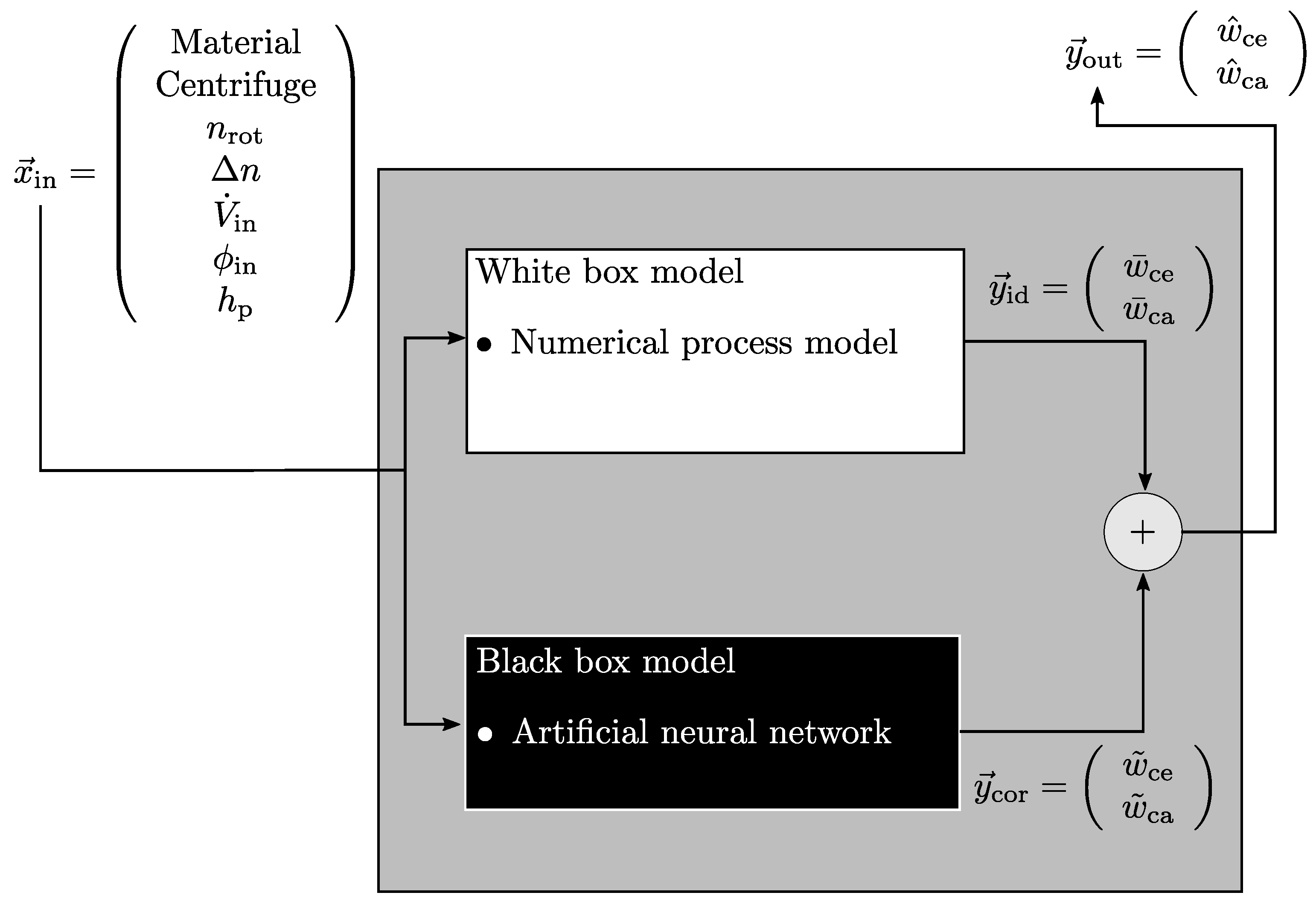
The grey box model used in this article is a stationary one and its structure is parallel, which is shown schematically in Figure 3.

The rotational speed $n_{\mathrm{rot}}$, differential speed $\Delta n$, volumetric flow rate ${\dot{V}}_{\mathrm{in}}$, solids volume fraction at the inlet ${\varphi }_{\mathrm{in}}$, and the pool depth $h_{\mathrm{p}}$ are used as input variables ${\overrightarrow{x}}_{\mathrm{in}}$. These represent typical process variables which are essential for the application of decanter centrifuges in the actual production process. The input variables are passed to the white box and black box. A numerical process model, as described in the previous section, is implemented for the white box model. Thus, this part represents the physical basis and serves as an ideal estimator for the simulated process. The simulated output ${\overrightarrow{y}}_{\mathrm{id}}$ consists of the solids mass fraction of the centrate ${\overline{w}}_{\mathrm{ce}}$ and cake ${\overline{w}}_{\mathrm{ca}}$. Furthermore, the black box is a neural network that corrects the simulation data according to the input variables and adjustment, if it is necessary. Adding the ideal, physical simulation result ${\overrightarrow{y}}_{\mathrm{id}}$ to the correction value ${\overrightarrow{y}}_{\mathrm{cor}}$ from the neural network,

$${\overrightarrow{y}}_{\mathrm{out}}={\overrightarrow{y}}_{\mathrm{cor}}+{\overrightarrow{y}}_{\mathrm{id}},$$

(3)

leads to the overall output ${\overrightarrow{y}}_{\mathrm{out}}$. In this case, the black box model is designed to potentially correct the white box model in the trained area. Therefore, summation is selected to combine both output components. Beyond the trained area, the grey box model only uses the white box model results. At this point it should be noted that in principle the grey box model may also be used in areas where the white box model would fail entirely, but, the focus of the study lies on the interpolative use, which is why it will not be discussed further. However, correction does not mean that the simulation results are unreliable and have to be corrected in all cases. 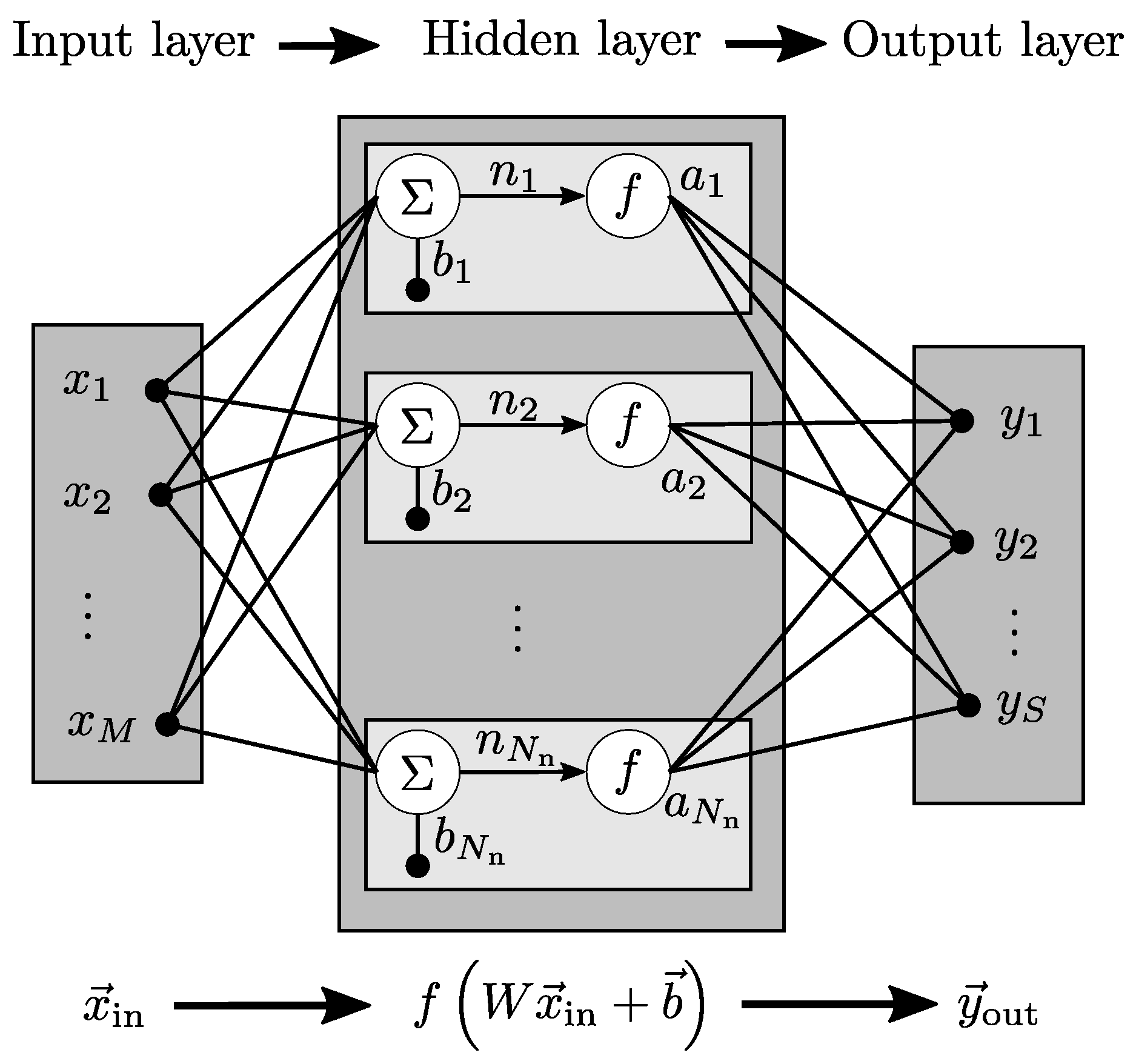In previous works [12,13,14] it was demonstrated that the method is indeed valid. Here, an enhancement must be created to consider effects that have not been modelled or to cover cases where no physical equations are known. The used neural network is a multilayer perceptron (a subcategory of feedforward networks) with an input and output layer and one hidden layer, which uses a sigmoid function as activation function. The number of neurons is optimised ($N_{\mathrm{N},\mathrm{opt}}=42$) via a bayesian optimisation and later varied from 3 to 50 to be discussed in the following section. The trained model can under- or overfit the data, since no physical equation is given as a basis, which determines the principal characteristics and trends of the data. Thus, underfitting means that the model does not adequately describe the trend of the data and overfitting means that the model captures almost every dependency including, for example, measurement inaccuracies, which is not a reasonable interpretation of the data. Therefore, a bayesian regularisation backpropagation algorithm is chosen to train the neural network. This technique includes a bayesian regularisation within the framework of the Levenberg-Marquardt algorithm [23]. It is specifically developed to have good generalisation capabilities [24,25] and to be practicable for limited training data access. Typically, the mean of the sum of squared network errors MSE is used during training of feedforward neural networks to evaluate the performance of the network. The MSE is defined as follows:

$$\mathrm{MSE}=\frac{1}{N_{\mathrm{td}}}\sum _{i=1}^{N_{\mathrm{td}}}{\left(e_i\right)}^2.$$

(4)

Here, $N_{\mathrm{td}}$ is the number of training data, $e_i$ is the network error. For a given number of neurons, the network adjusts the weights so that the MSE becomes minimal. With more neurons, the network tends to better reproduce the training data, which can lead to overfitting. This is reflected by the fact that the individual weights become relatively large. The evaluation function for the bayesian regularisation training algorithm is enhanced by the mean of the sum of squared network weights MSW,

$$\mathrm{MSW}=\frac{1}{N_{\mathrm{n}}}\sum _{j=1}^{N_{\mathrm{n}}}{\left(w_j\right)}^2,$$

(5)

where $N_{\mathrm{n}}$ is the number of neurons and $w_j$ are the weights of the neurons. This leads to the evalutation function for the bayesian regularisation training algorithm:

$$\mathrm{MSEREG}={\gamma }_{\mathrm{p}}\mathrm{MSW}+\left(1-{\gamma }_{\mathrm{p}}\right)\mathrm{MSE},$$

(6)

which combines the previously mentioned criterias MSE and MSW. The performance ratio ${\gamma }_{\mathrm{p}}$ balances both components and is automatically adjusted during training [24,25]. Thus, overfitting is additionally considered and penalised, which leads to the fact that this training algorithm has good generalisation capabilities.

Because of tolerances of the analytics, measurement devices, and sampling, the experimental data contain a specific measurement error. Similarly, the simulations include a trust interval influenced by assumptions made in the modelling. Therefore, a trust interval for the deviation between simulation and experiment is determined. If the deviation is within this tolerance, the remaining deviation is not modelled by the neural network. This should reduce the sensitivity for under- and overfitting additionally. The trust interval is $\pm 2$ $\mathrm{wt}.\%$ absolute for the deviation from the cake solids content and $\pm 1$ $\mathrm{wt}.\%$ absolute for the centrate. These values were determined due to the possibility of representative sampling. A variation of the trust intervals is discussed later in the results section.

Table 1. Value range and order of magnitude of used data set.

Variable	Value Range	Order of Magnitude
Rotational speed	1000 $\mathrm{rpm}$ to 3000 $\mathrm{rpm}$	103
Differential speed	15 $\mathrm{rpm}$ to 36 $\mathrm{rpm}$	101
Volumetric flow rate	500 $\mathrm{L}$ ${\mathrm{h}}^{-1}$ to 3000 $\mathrm{L}$ ${\mathrm{h}}^{-1}$	102 to 103
Solids content inlet	20 $\mathrm{wt}.\%$ to 30 $\mathrm{wt}.\%$	101
Pool depth	0.054 $\mathrm{m}$ to 0.094 $\mathrm{m}$	10−2
Solids content centrate	0 $\mathrm{wt}.\%$ to 30 $\mathrm{wt}.\%$	100 to 101
Solids content cake	50 $\mathrm{wt}.\%$ to 75 $\mathrm{wt}.\%$	101

lists the range and order of magnitude of the input variables with units.

For training, i.e., weighting of the individual nodes, it is more convenient that all data are of the same order of magnitude. Therefore, the dimensional data is normalised to the corresponding maximum value. As a result, the input values are always between zero and one. The correction parameter ${\overrightarrow{y}}_{\mathrm{cor}}$ has the unit $\mathrm{wt}.\%$ and can thus principally vary between 0 $\mathrm{wt}.\%$ and 100 $\mathrm{wt}.\%$. The variable called relative correction parameter in the following section is the correction parameter ${\overrightarrow{y}}_{\mathrm{cor}}$ related to 100 $\mathrm{wt}.\%$.

In this case, the data set consists of 62 individual data points. Each data point represents a parameter constellation between process variables and the output variables. Additionally, the individual data points are representative and informative. This means that they were determined to cover the required range of application and to be significant. In this case, the number of data points are few for the typical usage of neural networks. The measurement of the data points is associated with a significant experimental and time effort. Therefore, measurement data for parameter variations, as in this case, are only available to a limited amount from industrial practice. However, the flexibility of neural networks is a great advantage, which is why this methodology is used in this study. The neural network is intended to support a physically based white box model as a black box model in the concept of grey box modelling. The data set can also be easily extended with additional data points and the neural network can be retrained. This makes it possible to flexibly expand the range of applications. Typically, the data for neural networks is divided into training, testing, and validation data to determine the correct number of neurons and to avoid under- or overfitting. In this case, 50 data points (80%) were used for trainig, 6 data points (10%) for testing, and 6 data points (10%) for validation. The purpose is that the neural network is able to reproduce the data used. However, under- or overfitting can occur relatively easily and is therefore discussed in the results section. In this paper, the concept and methodology of grey box modelling is tested on the decanter centrifuge, where data is limited.

4. Results and Discussion

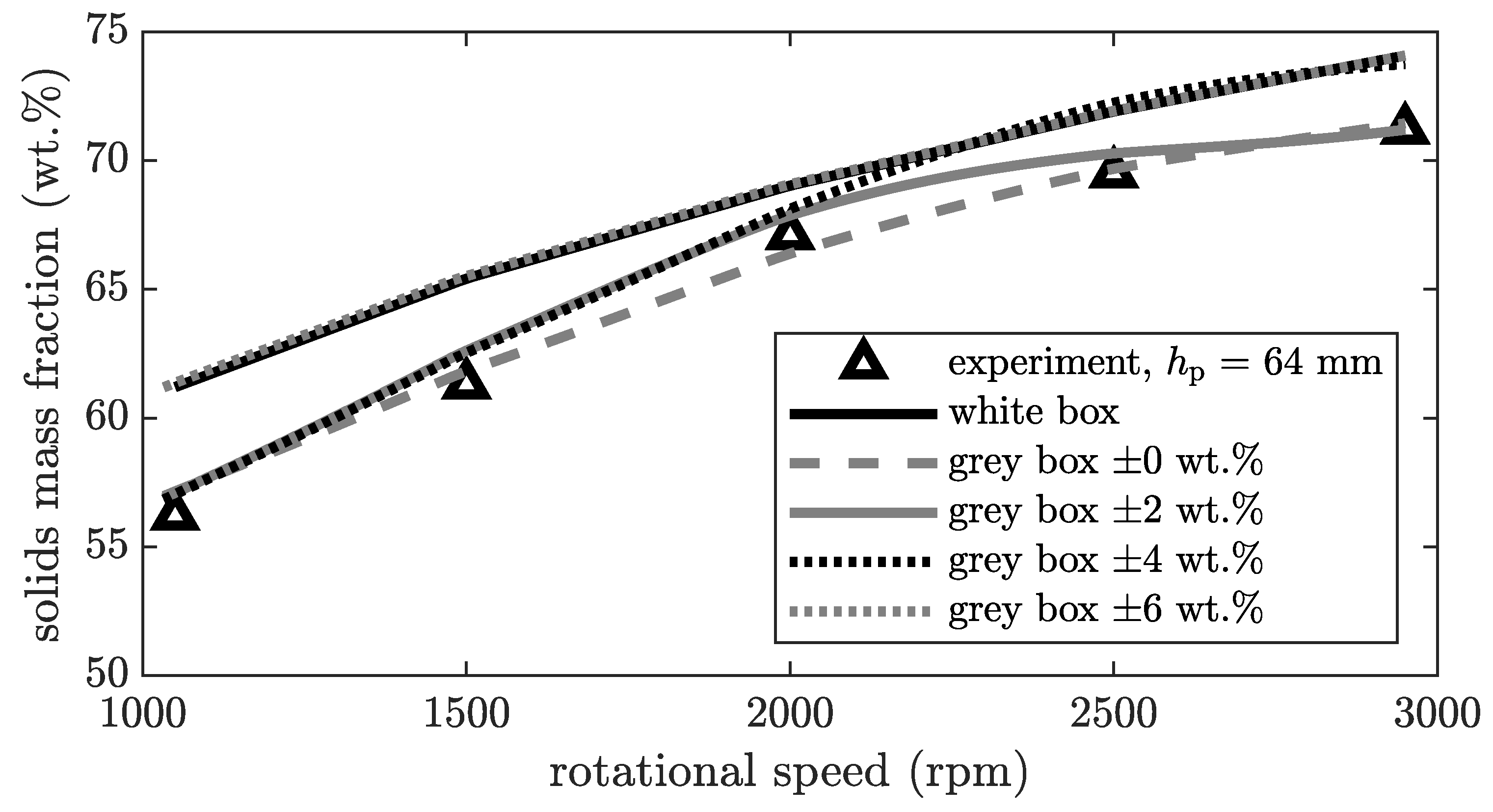
In this section, the settings of the neural network and validation of the training data are discussed. Figure 4 and Figure 5 are based on a neural network with 42 neurons. The influence of the number of neurons is discussed later (see Figure 6). In Figure 4, the solids mass fraction of the cake is plotted against the rotational speed for a constant pool depth $h_{\mathrm{p}}=64 \mathrm{m}\mathrm{m}$, volumetric flow rate at the inlet ${\dot{V}}_{\mathrm{in}}=2000 \mathrm{L} {\mathrm{h}}^{-1}$, and solids mass fraction at the inlet $w_{\mathrm{in}}=30\mathrm{wt}.\%$.

The trust interval varies between $0$ $\mathrm{wt}.\%$ and $\pm 6$ $\mathrm{wt}.\%$. As described previously, if the deviation between simulation and experiment is smaller than the trust interval, this deviation is not considered in the neural network. The output at the cake discharge represents a mean value over the whole sediment height. Based on preliminary tests, a trust interval of $\pm 2$ $\mathrm{wt}.\%$ is determined. This means that the experimental part the training data for the neural network can be determined with this precision. A trust interval of $0$ $\mathrm{wt}.\%$ means that the data can be measured perfectly and without error, which is not realistic and therefore not appropriate, although in this case the grey box model with a trust interval of $0$ $\mathrm{wt}.\%$ describes the results best. For the neural network, all measurement inaccuracies are modelled and thus lead to overfitting of the system. The opposite is a trust interval of $\pm 6$ $\mathrm{wt}.\%$ or even higher, meaning that the deviations between simulation and experiment are excluded and thus not modelled.

Figure 5 shows the solids mass fraction of the centrate as a function of the volumetric flow rate at the inlet for a constant rotational speed of $n_{\mathrm{rot}}=2950 \mathrm{rpm}$. The trust interval varies between $0$ $\mathrm{wt}.\%$ and $\pm 3$ $\mathrm{wt}.\%$.

Sampling for a representative sample is easier with centrate than with cake, as the centrate is typically more liquid and homogeneous. Therefore, the trust interval for the centrate is smaller and is determined to be $\pm 1$ $\mathrm{wt}.\%$. As mentioned above, a trust interval of $0$ $\mathrm{wt}.\%$ is not appropriate, because the experimental training data cannot be determined with this precision. All inaccuracies are modelled. However, there is no general rule or methodology to calculate the trust interval. It is a combination of the experimental error, which is calculable, and the quality of the simulations, which is difficult to quantify in detail. The quality of the simulation is about how much the simplifications and assumptions made during modelling affect the accuracy of the simulation result.

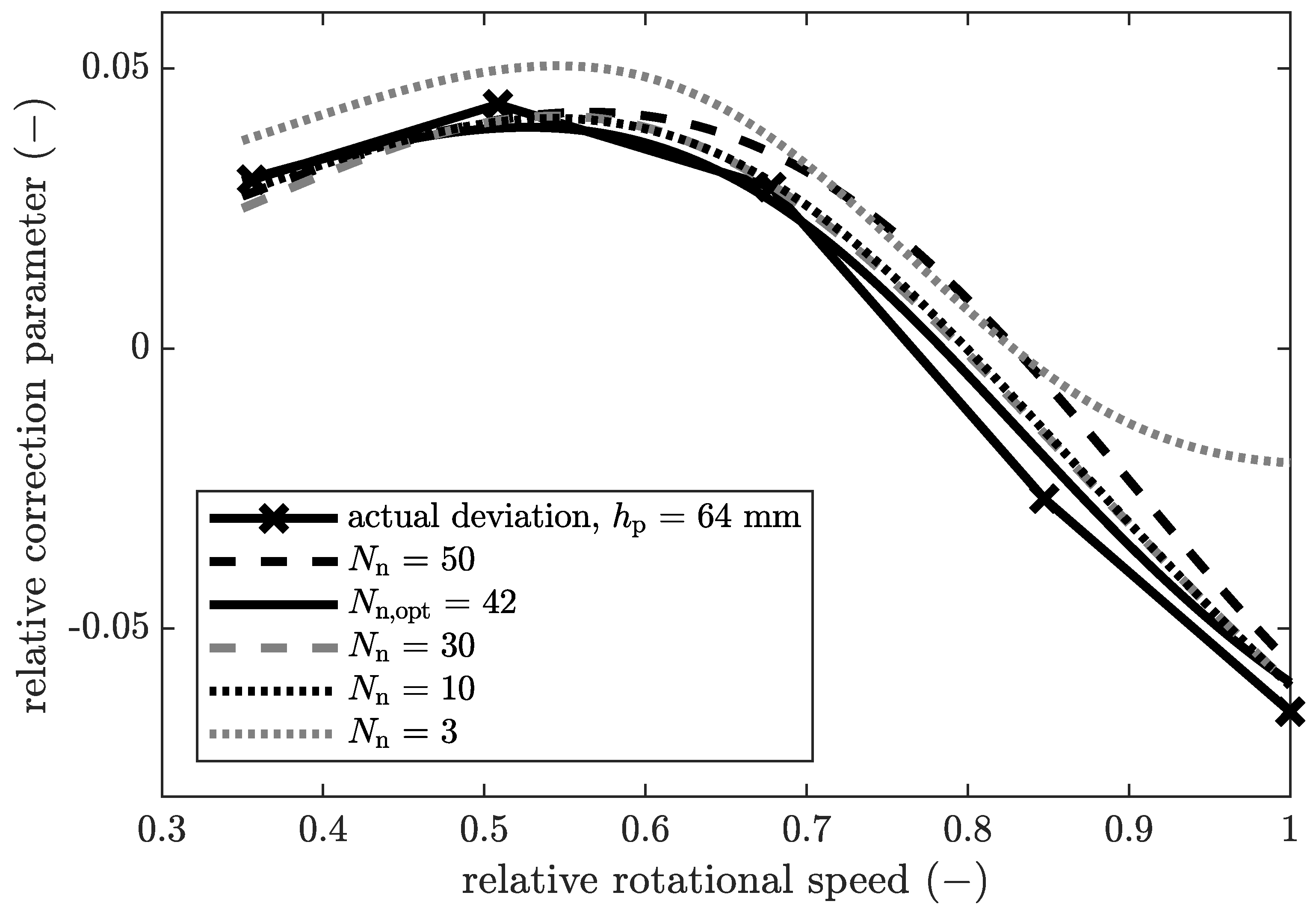
The analysis of a variation of the number of neurons in the hidden layer of the neural network is depicted in Figure 6. The relative correction parameter for the solids mass fraction of the centrate is shown over the relative rotational speed.

Here, the experimentally determined correction parameter is compared to the trained neural network. This selection represents only a part of the total amount of data. Nevertheless, it is exemplary for the in principle behaviour of this neural network. For all neural networks with ten or more neurons, the actual deviation can be modelled tendentially. However, differences in accuracy can be seen in certain sections. Between relative rotational speeds of $n_{\mathrm{rot},\mathrm{r}}=0.8$ and $n_{\mathrm{rot},\mathrm{r}}=1.0$, the graph for $N_{\mathrm{n}}=3$ deviates significantly from the experimentally determined data, which represent the actual deviation. For this network, the trend is not reproduced in this section. This indicates underfitting of this network. Typically, $N_{\mathrm{n}}=3$ is an extremely low value for the number of neurons. All other neural networks shown here map the training data very well. Furthermore, the curves do not show any overfitting. This is due to the bayesian regularisation backpropagation training algorithm that was developed specifically for this purpose.The number of neurons has only a minor influence on the quality and overfitting of the neural network in a wide range. Consequently, the model is more flexible in use, for example, when new data is included and the neural network needs to be retrained. This is a major advantage in engineering applications. By using Bayesian optimisation with neural networks [26], the optimal number of neurons could be obtained automatically. This optimisation algorithm compares the RMSE of all networks and selects the one with the minimal RMSE. Based on these results, the following validation is carried out with $N_{\mathrm{n},\mathrm{opt}}=42$ and a trust interval of $\pm 1$ $\mathrm{wt}.\%$ for the centrate and $\pm 2$ $\mathrm{wt}.\%$ for the cake of. In the following, the relative output of the black box model is shown in the upper graphs (a). The absolute output of the black box model is the difference between the white and grey box models and can therefore be derived in the graphs below (b).

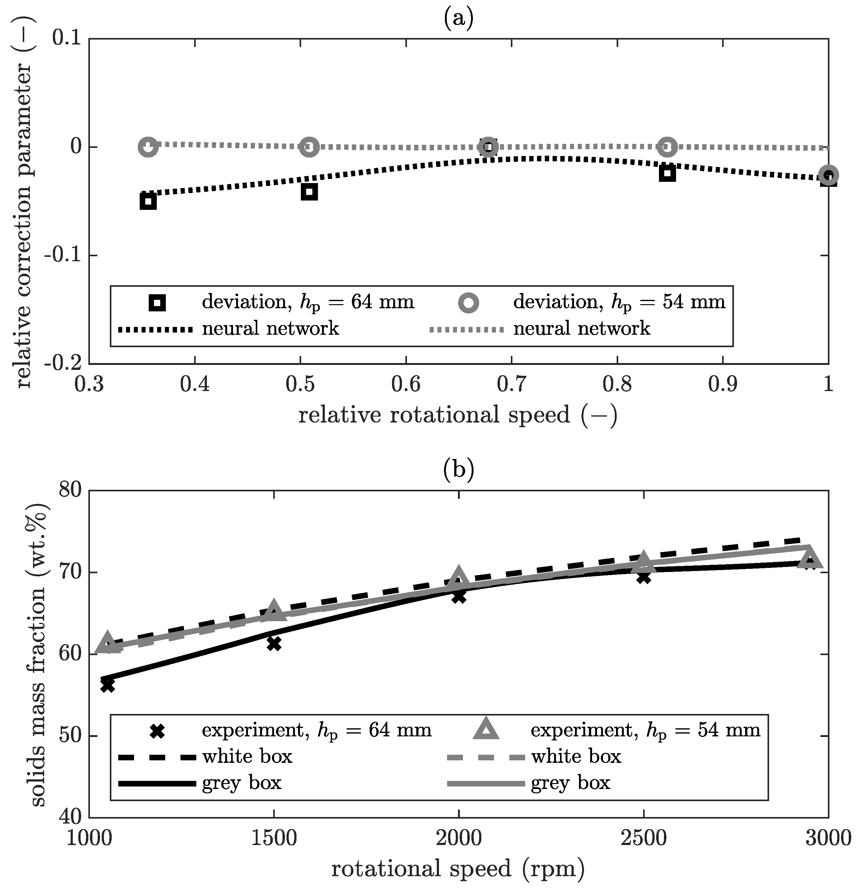
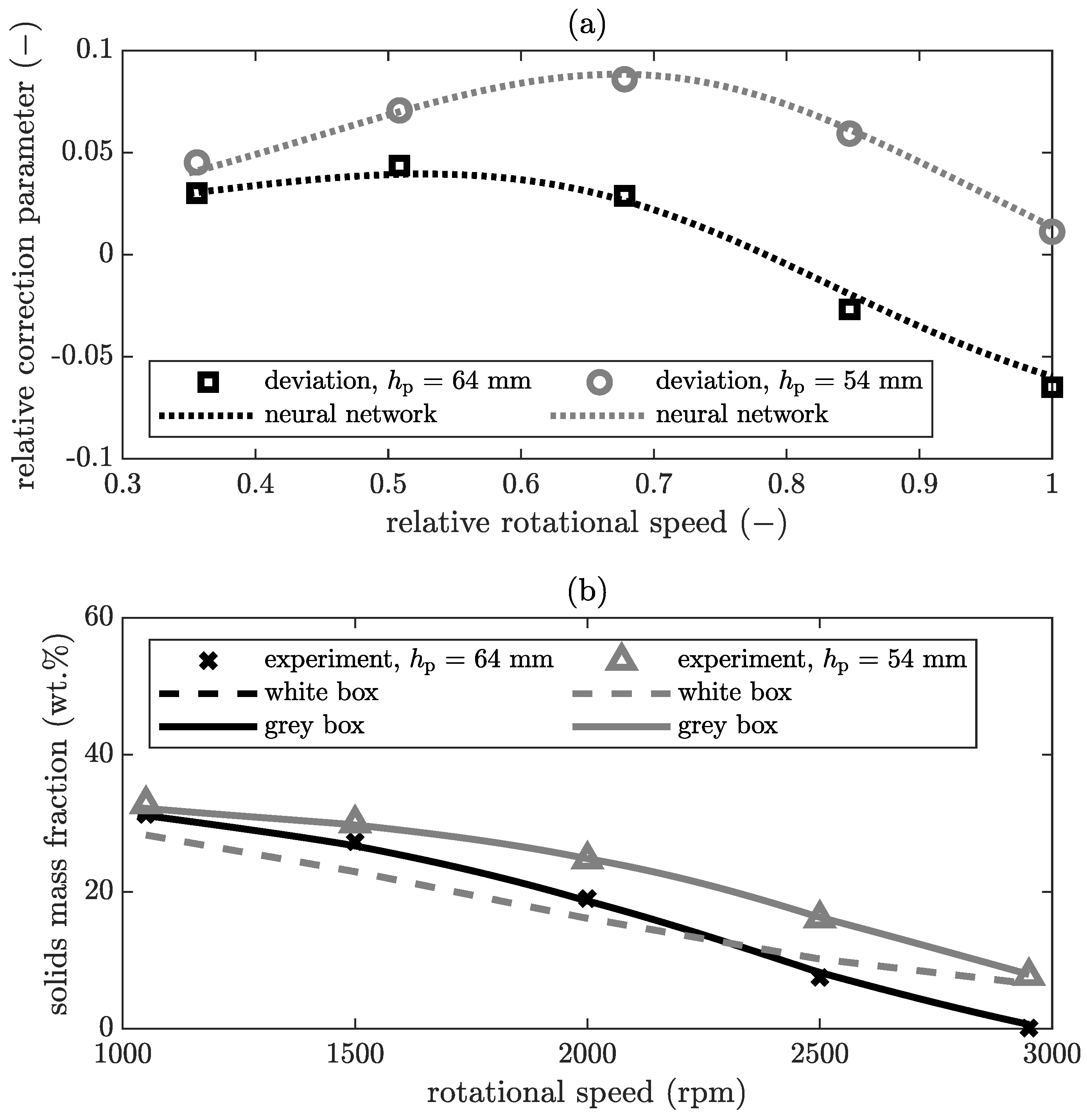
In Figure 7a, the relative correction parameter is plotted over the relative rotational speed for the solids mass fraction of the cake. On this basis, the simulation of the white box model is adjusted and results in the grey box model. In Figure 7b the corresponding result is compared between the experimental value, the result of the pure white box model and the grey box model.

The deviation function demonstrates that the neural network can model the actual deviation for this combination of parameters. For a pool depth of $h_{\mathrm{p}}=54 \mathrm{m}\mathrm{m}$, the deviations are within the range of the trust interval and are therefore not modelled. Thus, the results of the white and grey box model for a pool depth of $h_{\mathrm{p}}=54 \mathrm{m}\mathrm{m}$ in Figure 7b are similar. In the case of a pool depth of $h_{\mathrm{p}}=64 \mathrm{m}\mathrm{m}$, small deviations between white box model and experimental data exists which exceed the predefined trust interval. With the deviation function, the neural network describes these discrepancies to correct the white box model. As a result, the grey box model and white box model outputs differ in Figure 7b. Now, the grey box model represents the experimental data better than the white box model. However, the trust interval is defined by the user and depends on the preferences of the user. The measurement error of the experiments can be determined relatively easily in this case, but it is difficult to evaluate the accuracy of the simulation. For the same parameters as in Figure 7, the solids mass fraction in the centrate is displayed in Figure 8.

Here again, the upper diagram in Figure 8a demonstrates that the neural network describes the deviation. For both pool depths, the white box model follows the general trend that the solids mass fraction decreases with increasing rotational speed and the two white box models are basically equivalent, as the white box model is not sensitive enough to this difference in the pool depth. A more detailed discussion has been provided in previous publications with validation tests [12,14]. The experimental results reveal that for the same rotational speed, the solids mass fraction is higher at the smaller pool depth. Thus, the separation is better with increasing pool depth. However, the simulation shows no significant difference in the variation of the pool depth. There are several reasons for this. On the one hand, this is due to flow effects, such as the type of the developed flow, the effective pool depth, and the flow path due to the centrifuge geometry. This has an intensified influence if the pool is relatively deep and the centrifuge has a low degree of filling, which means that the volume flowing freely is tendentially larger. Leung et al. [27] assume that a so-called stagnant layer is formed on the surface under which the pool stands. This means that a particle is considered to be separated when it migrates out of the stagnating layer. However, there are contrary opinions in the literature about the conditions under which this stagnant layer is formed. Such flow phenomena affect the residence time behaviour of the particles. For this reason, the assumption of a developed plug flow along the entire pool depth up to the sediment surface for the calculation of the separation efficiency is not valid anymore. In this case, the root mean square error (RMSE) for a pool depth of 54 $\mathrm{m}$$\mathrm{m}$ is reduced from 6 $\mathrm{wt}.\%$ (white box model) to $0.33$ $\mathrm{wt}.\%$ (grey box model). For the pool depth of 64 $\mathrm{m}$$\mathrm{m}$, the reduction is from $4.14$ $\mathrm{wt}.\%$ to $0.51$ $\mathrm{wt}.\%$, which is in both cases a significant improvement.

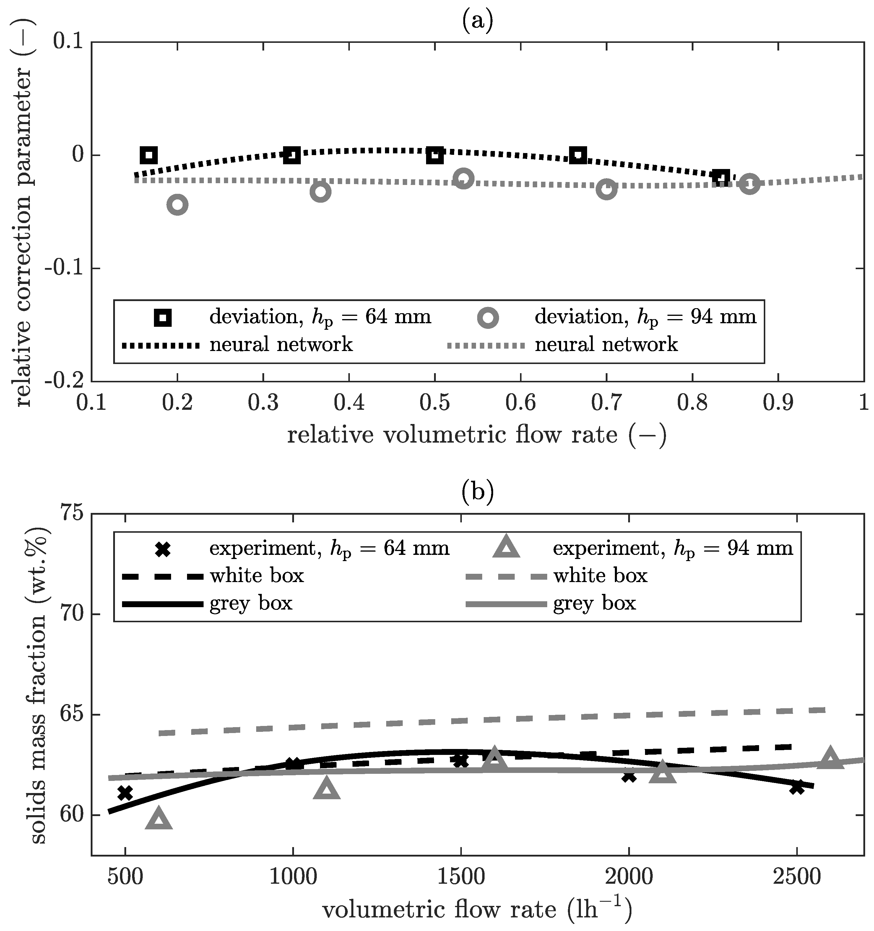
In Figure 9a, the relative correction parameter is plotted over the relative volumetric flow rate for a rotational speed of $n_{\mathrm{rot}}=2950 \mathrm{rpm}$. In Figure 9b the corresponding result is compared to the experimental value, the result of the pure white box model and the grey box model.

The deviation function demonstrates that the neural network can model the actual deviation for this combination of parameters. The influence of the volumetric flow rate on the solids mass fraction of the cake at a rotational speed of $n_{\mathrm{rot}}=2950 \mathrm{rpm}$ is minimal. Also, the influence of the pool depth is negligible. The white box model reflects this behaviour. Here, the neural network models only small deviations between experiment and white box model, since these are larger than the previously defined trust interval. The solids mass fraction for a volumetric flow rate between ${\dot{V}}_{\mathrm{in}}=1000 \mathrm{L} {\mathrm{h}}^{-1}$ and ${\dot{V}}_{\mathrm{in}}=2600 \mathrm{L} {\mathrm{h}}^{-1}$ is approximately constant for a pool depth of $h_{\mathrm{p}}=94 \mathrm{m}\mathrm{m}$. Therefore, the black box model corrects the white box model for this range with a factor that is approximately constant. The solids mass fraction at ${\dot{V}}_{\mathrm{in}}=600 \mathrm{L} {\mathrm{h}}^{-1}$ is $60 \mathrm{wt}.\%$, which is slightly lower than the other values for a pool depth of $h_{\mathrm{p}}=94 \mathrm{m}\mathrm{m}$. Due to the regularisation, the black box model is a compromise between the perfect reproduction of all training data and overfitting. As a result, the trend of this point is not clearly reproduced, as the other data are approximately constant at volumetric flow rates greater than ${\dot{V}}_{\mathrm{in}}=1000 \mathrm{L} {\mathrm{h}}^{-1}$. For example, if the trend of decreasing solids mass fraction at smaller volumetric flow rates (${\dot{V}}_{\mathrm{in}}<600 \mathrm{L} {\mathrm{h}}^{-1}$) continues, this might be modelled by the neural network if included in the training data set. For the same parameter as in Figure 9, the results for the centrate are plotted in Figure 10.

The experimental results indicate that the volume flow in this range between ${\dot{V}}_{\mathrm{in}}=500 \mathrm{L} {\mathrm{h}}^{-1}$ and ${\dot{V}}_{\mathrm{in}}=2600 \mathrm{L} {\mathrm{h}}^{-1}$ has no influence on the solids mass fraction in the centrate. In each case, the centrate is almost clear, which is equivalent to a solids mass fraction smaller than $0.1$ $\mathrm{wt}.\%$. This means that the centrifuge is not filled to the maximum capacity and there is still enough volume available for clarification. In general, if the volumetric flow rate increases further, the decanter centrifuge will reach its maximum capacity at a certain level, and separation will start to fail. The simulation results of the white box model already show a decrease in separation efficiency, which means an increase in the solids mass fraction in the centrate, starting at volumetric flow rate of ${\dot{V}}_{\mathrm{in}}=1500 \mathrm{L} {\mathrm{h}}^{-1}$. Therefore, the neural network has to correct the white box model. In this case, the RMSE for the pool depth of 64 $\mathrm{m}$$\mathrm{m}$ is reduced from $1.51$ $\mathrm{wt}.\%$ (white box model) to $0.34$ $\mathrm{wt}.\%$ (grey box model). For the pool depth of 94 $\mathrm{m}$$\mathrm{m}$, the reduction is from $1.84$ $\mathrm{wt}.\%$ to $0.24$ $\mathrm{wt}.\%$, which is in both cases an improvement. Particularly in this case, the improvement is of practical relevance, as it is obvious from this that the capacity of the centrifuge has not yet been reached as predicted by the white box model and that the volumetric flow rate can be increased further. This study did not investigate experimentally at which volumetric flow rate this maximum capacity level is reached. The grey box model is used in this work purely interpolatively. Outside the trained area, the white box model is considered correct. The intention is to improve exactly those domains in which the white box model is inaccurate. Nevertheless, the combination of white and black box model in extrapolation outside the trained domain is interesting and will be the subject of future investigations. As already described above, the white box model is based on the assumption that the flow regime is a plug-flow and flows directly towards the weir. The local separation efficiency is calculated by comparing the residence time with the settling time. At relatively deep pool depths, local eddies in the flow are possible in reality. This influences the residence time and would typically increase it, because the particles may circulate in the pool. With the same sedimentation time, the separation efficiency increases with increasing residence time. The white box model is unable to reflect this behaviour. However, the results of the grey box model show that by training the neural network, it can describe these deviations and thus represent this effect.

5. Conclusions

This article presents the development of a grey box model based on a dynamic process model and a neural network. The process model alone cannot map local flow effects on the separation behaviour at rather deep pool depths, because this would require detailed CFD simulation. Therefore, the parametric model is combined with a neural network which is trained with selected data to represent these dependencies. This extends the application range of the numerical process model without losing the advantages of a process model. Generally, this provides new possibilities to extend the simulation tool. Additional effects can either be integrated into the parametric model using further equations or the neural network learns to map the correlations by means of specific experiments.

In the next step, the presented stationary grey box model is adapted to a dynamic one with respect to the increasing sensorisation of machines in production environments. Thus, the accuracy of the model can be increased, if the data is trustable, representative, and informative. Grey box modelling clearly is a very useful application in the context of increasing digitalisation. In addition, it is conceivable to use detailed CFD simulations instead of specific experiments to train the ANN. This reduces the experimental effort and goes one step further in the direction of digitalisation. As a result, the grey box model has the advantage of a dynamic process model in terms of computing time but also in terms of a significantly increased accuracy.