Abstract
Centrifugal air classifiers are often used for classification of particle gas flows in the mineral industry and various other sectors. In this paper, a new solver based on the multiphase particle-in-cell (MP-PIC) method, which takes into account an interaction between particles, is presented. This makes it possible to investigate the flow process in the classifier in more detail, especially the influence of solid load on the flow profile and the fish-hook effect that sometimes occurs. Depending on the operating conditions, the fish-hook sometimes occurs in such apparatus and lead to a reduction in classification efficiency. Therefore, a better understanding and a representation of the fish-hook in numerical simulations is of great interest. The results of the simulation method are compared with results of previous simulation method, where particle–particle interactions are neglected. Moreover, a validation of the numerical simulations is carried out by comparing experimental data from a laboratory plant based on characteristic values such as pressure loss and classification efficiency. The comparison with experimental data shows that both methods provide similar good values for the classification efficiency d50; however, the fish-hook effect is only reproduced when particle-particle interaction is taken into account. The particle movement prove that the fish-hook effect is due to a strong concentration accumulation in the outer area of the classifier. These particle accumulations block the radial transport of fine particles into the classifier, which are then entrained by coarser particles into the coarse material.
1. Introduction
Centrifugal classifiers are used for classification of particle gas flows due to their good classification efficiency and wide range of applications, especially in the pharmaceutical, food, coal, and cement industries [1,2,3,4,5]. Evaluation parameters for the classification properties of a classifier are the classification efficiency d50, which indicates at which particle size 50% each ends up in the fine and coarse product, and the classification selectivity κ, which results in d25/d75. The particles are classified by the rotating blades in the classifier, which generate a forced vortex, causing the particles to experience a centrifugal force acting against the direction of flow. Coarse particles are thus rejected at the outer edge of the classifier, while fine particles follow the air flow inwards and enter the fines [6]. In order to better understand the classification mechanism and to optimize the geometry with respect to energy efficiency, a number of experimental and numerical studies have been carried out in the past. Many numerical studies so far have had the goal of investigating and optimizing geometric influences such as the horizontal and vertical classifiers or the structure of the classifying wheel blades in more detail [7,8,9,10,11,12,13]. As a general practice, the resulting velocity and pressure profiles were determined without taking particle–particle interactions into account and particle trajectories in the classifier were derived. In some cases, even the influence of the solid load on the flow was neglected. These simplifications were chosen due to the complexity of the classifier resulting in a high computational effort. In some cases, these simplifications are justified by the fact that only low solid loads are present and the influence of the particles is negligible [10,14]. The comparison of experimental and numerical separation efficiency confirms these assumptions. However, some studies declare that the solid load has an influence on the separation efficiency in a classifier [8]. Probably the influence of the solid load depends on the design of the classifier and the process conditions. Moreover, the fish-hook effect, which often occurs in the classifier, could not be reproduced in simulations. The fish-hook effect, which owes its name to the characteristic curve of the separation efficiency, is shown in Figure 1. Since more particles enter the coarse material as the particle size decreases, the curve rises sharply in this area, causing large portions of the fine material to enter the coarse material and significantly reducing the yield of a classifier. For this reason, it is of interest to better understand the processes that lead to the fish-hook effect and to represent them numerically.
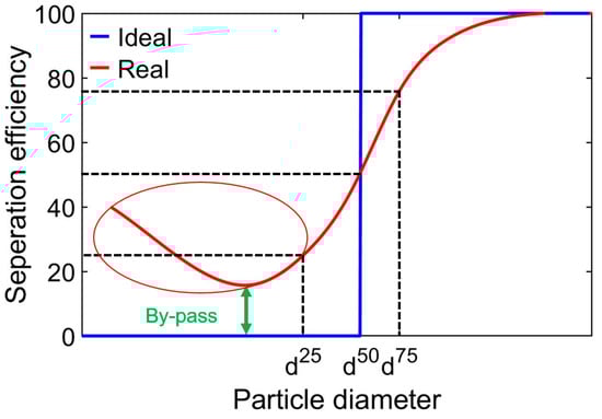
Figure 1.
Cut size, fish-hook, and by-pass.
Various researchers have attempted this so far, not only for centrifugal classifier but also for similar apparatus like cyclones. Nagaswararao et al. [15] summarize previous studies and draw the following conclusion. There is no uniform consensus in literature for the occurrence of the fish-hooks effect. Generally, two effects are held responsible for it. In the first theory, the fish-hook effect is based on the entrainment of fine particles in the boundary layer of coarser particles. In the second theory it is assumed that fine particles acquire velocities larger than the Stokes velocity when entrained by coarse particles [16]. In addition, the fish-hook effect occurs more frequently in measurements when the sizing analyses are carried out by Laser diffractometry using his optical mode [15].
In centrifugal classifiers, however, only a few studies on the fish-hook effect are available. The flow profile in a centrifugal classifier is similar to a cyclone but not the same. Firstly, Eswairah et al. [17] blame the fine particles’ rebound in the classifier’s blades, Guizani et al. [18] consider secondary recirculation flows and bubble-like vortex decay inside the classifier. Eswairah et al. [17] support their results with sieve curves in which the fish-hook effect is measured in a classifier. Furthermore, Barimani et al. [19] adopted a new approach to study the fish-hook effect. By focusing the investigations on a periodic section of the classifier, the relevant regions in front of and between two classifying wheel blades were resolved in more detail. Using the Discrete Phase Model (DPM) particle trajectories of particles of different sizes were then determined and conclusions were drawn about the concentration and residence time of different particle sizes in the classifier. This proved that there is a strong accumulation of particles of similar cut size in the classifier directly in front of the classifier wheel blades. According to Barimani et al., the accumulations ensure that the solids concentration upstream of the classifier is many times higher than previously assumed and exceeds the feed concentration many times over. Furthermore, they derive that these increased solids concentrations intensify the interaction of especially very small particles with larger particles and thus inhibit the radial movement of the very fine particles into the interior of the classifier. However, a proof of this assumption has not yet been achieved, since consideration of particle-particle interactions has always been neglected in the previous simulations.
When simulating a multiphase solid-fluid flow in a classifier, the Euler–Lagrangian approach is suitable. In this article, the Euler phase is modelled with the continuum Navier Stokes equations, while the particles are modelled as Lagrangian elements with fixed properties such as diameter and density. A fully coupled (4-way) Euler–Lagrangian approach includes the momentum transfer between the two phases as well as a consideration of particle-particle interactions. Since a detailed resolution of each individual collision for densely charged air flows is very computationally intensive, the multiphase particle-in-cell (MP-PIC) method is used for the first time in this work. In the MP-PIC method, particle–particle interactions based on averaged particle stresses derived from the Lagrangian approach are transferred to the Eulerian network, which means that the particle collisions do not have to be resolved directly. The modelling of the particle collision using the Eulerian mean values and the parcel concept, in which several particles with the same properties are considered as one parcel, make the MP-PIC method suitable for dense particulate flows without a significant loss of accuracy [20].
Therefore, this new solver allows for the first time the consideration of particle-particle interaction in a 3D simulation for classifiers. The results are compared with results without considering particle–particle interactions and validated with experimental data. Furthermore, the effects of the solid load on the flow profile are examined in more detail.
2. Materials and Methods
2.1. Apparatus Description
Figure 2 shows the laboratory plant provided for the validation of the numerical model. The particles are fed into the apparatus from above onto a deflector plate, which introduces the particles into the system between static guide blades and the classifier. The air flow introduced via a tangential inlet conveys the particles through the classifier into the fine product, where they are then separated from the air with the help of a cyclone. The particles separated at the classifier due to centrifugal forces are held in the periphery of the classifier between static guide vanes and the classifier until they sediment downwards due to gravity and enter the coarse product. The material that reaches the coarse or fine material is weighed and sampled. A Mastersizer 2000 from Malvern Panalytical then measures the particle size distributions using laser diffraction. Material properties of the solid and the air as well as characteristic sizes of the classifying wheel are presented in Table 1. The pressure drop is determined between the point in front of the static blades and at the outlet of the classifier.
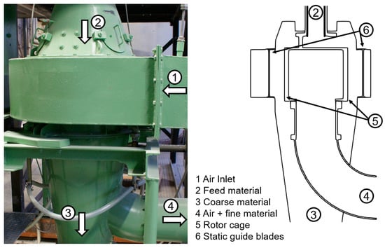
Figure 2.
Schematic representation of the laboratory plant.

Table 1.
Characteristic sizes of material, air, and classifier wheel.
2.2. Numerical Methodology
2.2.1. Governing Equations
In the following, the general equations that serve as the basis for the numerical solver are described. The equations are based on the assumption that the flow is incompressible and isothermal. For the fluid phase, since the solver is based on a Euler–Lagrange approach, the Navier–Stokes equations are solved, in which an influence of the solid phase is taken into account. The volume fraction of the continuous phase results in
where is the volume fraction of the solid phase and is expressed according to
from the individual particle volumes in a grid cell. The continuity conservation equation then becomes
and the momentum equation is given by
with the interphase momentum transfer given by
and the mass of the solid particle , the density of the fluid , the density of solid particle , the velocity of the fluid , the pressure of the fluid , the velocity of the solid particle , the fluid stress tensor , the gravity vector g, and the particle volume . The particle distribution function f depends on the particle position , the particle velocity , the particle mass , and the time t define the evolution of the particle phase, which is expressed by a Liouville equation:
where is the particle acceleration, given by
The interparticle stress includes particle–particle interactions with each other and must be taken into account in the MP-PIC method for particle acceleration. The first three terms are the drag force, the force due to a pressure gradient within the fluid and gravitational force. Other smaller forces such as virtual mass, Basset or lift forces are neglected. The continuity and momentum equations for the particulate phase result from the multiplication of and with Equation (5) and an integration over particle volume, density, and velocity. These terms are not presented here, as they are already described in detail in the literature [19,20].
For the interparticle stress, the model by Harris and Crighton [21] applies, which is described in Equation (8)
where is the solid pressure constant, β is an empirical constant, is the volume fraction of the dispersed phase at close packing, and ε is a small number to satisfy numerical stability. The model by Harris and Crighton does not include direct consideration of velocity differences between particles. At first, this seems to be a major disadvantage, as particles that are rejected at the classifier have significantly higher velocities after particle-wall collision with rotating components than entering particles. However, it must be emphasized that if a particle cloud is formed in front of the classifier wheel, this error is mitigated, since the majority of particles move around the classifier wheel at similar velocities and, secondly, the fish-hook effect is presumably due to the fact that small particles never get between two classifier wheel blades, since otherwise they would almost certainly enter the fines. This steric hindrance should be well reproduced by the Harris–Crighton model. Furthermore, it is numerically very stable.
In the MP-PIC method, the influence of particle-particle interaction can be subdivided into sub-models. The most important ones are packing models [22] collision damping models [23] and collision isotropy models [24]. In this study, the explicit packing model and the stochastic collisional isotropy model, which are already implemented in OpenFoam are applied. No collision damping model was considered because it leads to unrealistic particle movements. The drag force contained in the interphase momentum transfer term is taken into account with a combination of the models by Ergun [25] and Wen-Yu [26], both of which are known to be well-suited for density-charged particle flows. If the continuous phase fraction is less than 0.8, the Ergun model is exercised. Particle–wall interactions are described using a simple impact model with restitution coefficients. For the fluid simulation, Reynolds-averaged Navier–Stokes (RANS) equations is used as a turbulence model along with Menter’s shear stress transport (SST) turbulence model [27]. The individual parameters for the models used are shown in Table 2. The values were adjusted in the simulation to fit as well as possible with the experimental data. The effect of turbulence for particles is taken into account by applying stochastic dispersion model from OpenFoam-6. Therefore, the velocity is perturbed in random direction, with a Gaussian random number distribution.
Table 2.
Main numerical parameters.
Since the classifier is a rotating part, an MP-PIC solver based on the software environment OpenFOAM-6 is extended with the multi-frame of reference (MRF) model. In the MRF model, the numerical cells of the rotating part are supplemented with additional centrifugal and Coriolis forces. The rotating part is frozen in a fixed position; an exchange surface between the different frames of reference is applied. This approach requires that the particle forces be calculated according to the zone. If a particle is inside the classifier in the rotating section, the relative velocity of the fluid is taken into account to calculate the particle forces, if a particle is in the stationary section outside the classifier, absolute velocities are considered. This is necessary because the rotating wall does not rotate in the simulation and a particle therefore only moves at the relative velocity to the rotating wall. This model works well and has already proven itself in other studies due to its short computing time and robustness [28]. However, it has never been combined with the MP-PIC method. For this purpose, the calculation of the interparticle stress term also had to be adapted. This is calculated with absolute velocities of fluid and particle, but its effect is adjusted for the rotating zone. The solver is adapted in this respect.
2.2.2. Simulation Conditions
Two properties influence the creation of the grid when applying the MP-PIC method. On the one hand, the flow requires a good resolution of the flow area, on the other hand, the grid cells are larger than the particles. Furthermore, the accuracy increases if a sufficiently large number of particles are present in a grid cell, since the numerical instability increases with strongly fluctuating volume fraction. For this reason, only a periodic section of the classifier is examined in the geometry under investigation. This significantly reduces the number of grids and the number of particles per volume can be significantly increased. In reality, there is no complete rotational symmetry due to the tangential flow inlet of the air, but investigations on the 360° geometry have shown that the high solid loads between the static guide vanes and the classifier cause a uniform distribution of the airflow over the radius.
Figure 3 shows the geometry with the boundary conditions. At the air inlet, the volume flow corresponds to the volume flow in the experiments. At the outlet, an absolute constant pressure of 0 Pa is set. The walls have a standard no-slip boundary. Since both the solids feed and the coarse material discharge are airtight, these are also assumed as walls. In addition, the discharge of coarse material is significantly reduced, as it can be adopted that particles that have exceeded the lower edge of the classifier will enter the coarse material. An uneven distribution of the solids flow as well as particle velocities due to the baffle plate are neglected, so that the particle feed takes place uniformly without velocity. The averaged value of y+ is 10 for the blades of the classifier and 5–7 for all other walls. A full resolution of the boundary layer requires a y+ value of 1 and therefore, a significant number of additional cells. That is why a y+-wall function is used to model the near-wall turbulence. This is a good compromise between accuracy and computational costs.
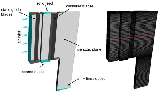
Figure 3.
3D domain, boundary types, and CFD grid.
To investigate the sensitivity of the grid, three different grids are investigated. Table 3 compares the pressure drop from the simulation with experimental data for the three grids. The comparison is at a classifier speed of 900 rpm. The standard deviation is calculated to pressure loss in experiment for all grids.
Table 3.
Comparison pressure drop for three grids between simulation and experiment at a classifier speed of 900 rpm.
The grid used is the medium grid, which consists of a hexahedral mesh with 304,222 cells. It is shown on the right-hand side of Figure 3. The grid is a good compromise between accuracy and calculation time. The left-hand side of Figure 4 plots the contours of the static pressure on the periodic surface and an axial section through the apparatus. The axial section is made through the red line in Figure 3. The figure shows that the pressure inside the classifier drops dramatically. This is due to the fact that the tangential velocity inside the classifier first increases considerably with smaller radius and then drops drastically. The flow profile is comparable to a cyclone and described in detail by Toneva et al. [29] and also a proof for the correctness of the simulations. In addition, the pressure loss between experiment and simulation is compared on the right-hand side of Figure 4. In the simulations, the pressure loss is underestimated by about 10% compared to the experimental data, what is a satisfactory result. The deviations are probably due to simplifications in the geometry.
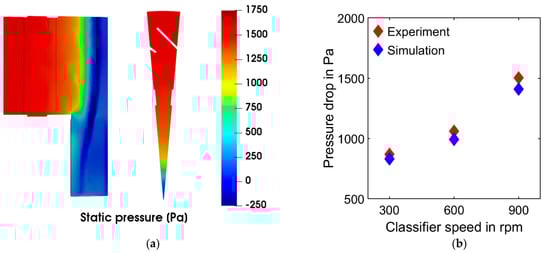
Figure 4.
(a) Contours of static pressure at a classifier speed of 900 rpm; (b) comparison pressure drop between experiment and simulation.
3. Results
3.1. General Flow Profile in Classifier
At the beginning, the general flow profile in the classifier is discussed. From this, it is possible to better understand the movement of the particles. The particle separation takes place between the classifier blades. For this purpose, Figure 5 shows an axial section, see red line in Figure 3, through the classifier and the radial and tangential velocity profiles in front of and between two classifier blades.

Figure 5.
Contours of velocity in front of and between classifier blades at a classifier speed of 900 rpm and no solid load (a) radial component; (b) tangential component.
The velocities shown are at a speed of 900 rpm and at clockwise rotation. The outer edge of the classifier rotates at a tangential velocity of 15 m/s. The tangential velocities in front of the classifier are significantly lower than between the classifier blades, which means that the leading blade acts as a tear-off edge and a dead zone forms between the classifier blades. This dead zone constricts the radial air transport into the interior, which means that there is no uniform radial velocity profile between the classifier blades. Negative radial velocity means that the air flows towards the center inwards, positive velocity transports air outwards. The formation of the dead zone depends on the rotational speed of the classifier and becomes larger as the rotational speed increases. This is due to the fact that as the classifier speed increases, the difference in velocity between inside the classifier blades and outside becomes greater and greater. This is shown in left-hand side of Figure 6 in more detail. There the radial velocity for three different classifier speed is shown. The right-hand side of Figure 6 illustrates the influence of the solid load on the radial velocity between the classifier blades. The solid load equalizes the radial velocities and reduces the formation of the dead zone with positive radial velocities.
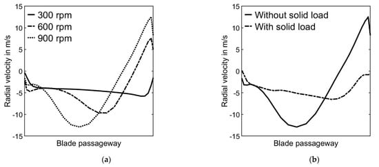
Figure 6.
(a) Radial velocity between classifier blades for three different classifier speeds with no solid load; (b) radial velocity between classifier blades with and without solid load at 900 rpm.
3.2. Particle Movement in Classifier
The particles entering the classifier have significantly lower tangential velocities than the rotating classifier wheel due to the low air tangential velocities in front of the classifier. Therefore, particles entering the classifier blades collide with the trailing blade. The left-hand side of Figure 7 sketches the distribution of the particles and their size in front and between the classifier blades in 2D. There, smaller particles are marked blue, larger particles are shown in red. The figure illustrates that above all small particles enters the classifier blades and then collide with the trailing the blades.
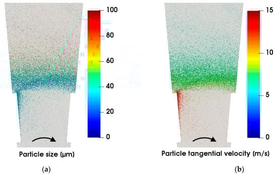
Figure 7.
(a) Particle size in front of and between classifier blades at 900 rpm; (b) particle tangential velocity in front of and between classifier blades at 900 rpm.
The right-hand side of Figure 7 shows the tangential velocity of the particles. This demonstrated that the particles colliding with the trailing blade are accelerated by the classifier and have significantly higher velocities after impact. The particles accumulate primarily on the trailing blade. Fine particles are now transported further into the fine material, while coarse particles are pushed outwards by centrifugal force. The particles rejected at the classifier accumulate directly in front of the classifier wheel and move on a circular path around the classifier. They have significantly higher tangential velocities than particles on the circular path outside the classifier. Accordingly, they collide with the particle cloud as they exit, which slows them down again considerably. The particle cloud moving on a circular path in front of the classifier also prevents the transport of “new” particles into the classifier. In addition, the angle of entry depends on the speed of the classifier.
The entry angle of the particles between the classifier blades depends on several factors. Firstly, it depends on the particle size. Small particles are accelerated faster by the high tangential air between the classifier blades than coarse particles and therefore reach further inwards between two classifier blades bevor colliding with the trailing blade. Figure 8 illustrates schematic the difference particle path between a small and a coarse particle. In reality, the greatest wear is detected at these points in the apparatus, which supports the plausibility of the calculated trajectories.
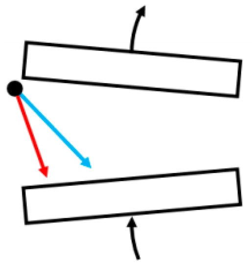
Figure 8.
Schematic of particle path between classifier blades for a small particle in blue and a coarser particle in red.
Figure 7 shows that small particles that would actually enter the fines due to their size do not pass through the cloud between the classifier wheel blades. At this point, it must be mentioned that the particle impact model used is subject to a fundamental assumption. The influence of different particle velocities is only taken into account to a limited extent. It can be assumed that particle-particle collisions, which would accelerate particles to very high velocities, are thereby weakened. In reality, it is quite possible for large particles to receive a high velocity component inside the classifier and enter the fine material. The impact model used here therefore tends to support ideal separation.
In the following, more attention is focused on the axial particle transport. Figure 9 shows the particle distribution in the apparatus at two different time steps in simulation. The particles are all shown in the same size, small particles are colored blue, larger particles are colored red. If one compares the two figures, it is noticeable that the particles are primarily located between the static guide vanes and the classifier. In this area, denser particle clouds repeatedly form, which then sediment downwards into the coarse material as a particle swarm. The swarm sedimentation is a non-stationary process, which is illustrated by the two time steps. Very small particles, in the order of <60 µm, reach the fine material over the entire classifier height. At the same time, however, fine particles accumulate in denser particle clouds and are carried down with them and can also enter the coarse material. This can also be seen in the separation efficiency curves shown in the left-hand side of Figure 10.
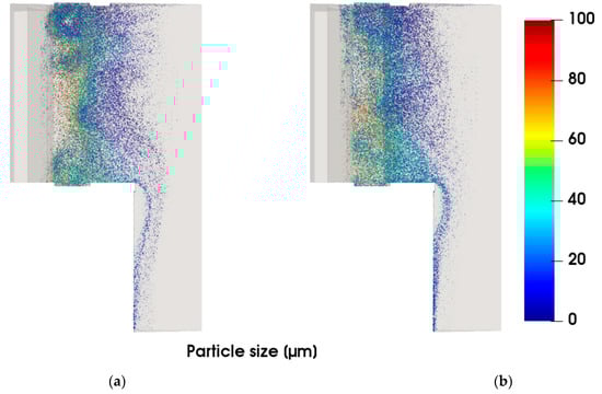
Figure 9.
Unsteady particle movement in the apparatus at two different times at 900 rpm; (a) after 15 s; (b) after 20 s.
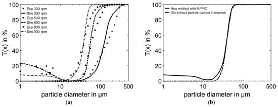
Figure 10.
(a) Comparison of the experimentally measured and simulated collection efficiency with the new solver at three different classifier speeds; (b) comparison of the simulated collection efficiency with new method based on MPPIC and old version without particle-particle interaction at 900 rpm.
The separation efficiency curves from the experiments and the simulations for three speeds are compared. As expected, the separation efficiency curve is shifted to the left as the classifier speed increases, since fewer and fewer particles enter the fines as the centrifugal force increases. The simulated curves reflect this effect well and the calculated d50 values also deviate only very slightly from the experimental data. In the experimental tests, the fish-hook effect only occurs above a speed of 600 rpm; it is not observed at lower speeds. This can be attributed to the fact that at high classifier speeds, more particles are rejected at the classifier and the particle concentration in front of the classifier increases as a result. In the simulations, the fish-hook effect only occurs at 900 rpm. Nevertheless, the simulations allow the fish-hook effect to be proven and can depict it in a weakened form. Furthermore, the simulated separation efficiency curves are sharper, which is probably due to the particle-particle interaction model used, as mentioned above. Furthermore, periodicity is assumed in the simulation. Due to only one air inlet and a possibly inhomogeneous particle feed, it is quite realistic that poorer classification selectivity occurs in the experiments. The right-hand side of Figure 10 compares the new method presented here that takes particle interactions into account and a solver that does not take particle interactions into account. Both solvers provide similar separation degree curves, but the fish-hook effect is only reproduced by the new solver. This is also confirmed by Table 4 in which the classification efficiency d50 and classification selectivity κ are qualitatively compared for both numerical methods with experimental results.
Table 4.
Comparison classification efficiency d50 and classification selectivity κ in experiment, new method with MPPIC and solver without particle-particle interaction.
4. Discussion
In this paper, a new solver for simulating the particle gas flow in a centrifugal classifier is presented and validated against experimental data from a laboratory plant. Based on the MP-PIC method, the solver allows for the first time the estimation of the influence of particle-particle interactions on the classification process in 3D case. Therefore, the flow profile, particle movement and separation process in the classifier can be described in more detail.
It is proven that particles rejected at the classifier accumulate more in front of the classifier and sterically block the radial transport of other particles. As a result, fine particles do not reach the inside of the classifier and are dragged into the coarse material by coarse particles. To reduce the fish-hook effect, therefore, the formation of the particle cloud in front of the classifier would have to be prevented, maybe by installing flow baffles in front of the classifier. Furthermore, it is shown that particle cloud formation in front of the classifier is discontinuous and that high load fluctuations occur in front of the classifier. In addition, the fish-hook effect is mapped in simulations for the first time and its development process is thus resolved. This shows a comparison with simulations without particle-particle interaction in which the fish-hook effect is not reproduced.
However, the fish-hook effect only appears in the new simulation method in a weakened form at higher classifier speeds. This is possibly due to the limiting of the solver, especially the approach that parcels are simulated instead of particles due to the immense computing time or that the impacts are not fully resolved. Nevertheless, the calculated results well represent characteristic parameters of the classifier such as the pressure loss and the classification efficiency d50.
In further steps, the validation should be continued, and the solver should also be compared with experimental results for other classifier types and process conditions. In addition, other models should be tested instead of the Harris and Crighton model.
Author Contributions
Conceptualization, M.B.; Formal analysis, M.B..; Investigation, M.B.; Methodology, M.B.; Project administration, M.B.; Software, M.B.; Supervision, H.N. and M.G.; Validation, M.B.; Visualization, M.B.; Writing—original draft, M.B.; All authors have read and agreed to the published version of the manuscript.
Funding
This research received no external funding.
Data Availability Statement
Not applicable.
Acknowledgments
We acknowledge support by the KIT-Publication Fund of the Karlsruhe Institute of Technology.
Conflicts of Interest
The authors declare no conflict of interest.
Abbreviations
The following abbreviations are used in this article:
| CFD | Computational Fluid Dynamics |
| DPM | Discrete Phase Model |
| MP-PIC | Multiphase particle-in-cell |
| MRF | Multi-frame of reference |
| RANS | Reynolds-averaged Navier–Stokes |
References
- Shapiro, M.; Galperin, V. Air classification of solid particles: A review. Chem. Eng. Process 2005, 44, 279–285. [Google Scholar] [CrossRef]
- Batalović, V. Centrifugal separator, the new technical solution, application in mineral processing. Int. J. Miner. Process 2011, 100, 86–95. [Google Scholar] [CrossRef]
- Johansen, S.T.; de Silva, S.R. Some considerations regarding optimum flow fields for centrifugal air classification. Int. J. Miner. Process 1996, 44–45, 703–721. [Google Scholar] [CrossRef]
- Wang, X.; Ge, X.; Zhao, X.; Wang, Z. A model for performance of the centrifugal countercurrent air classifier. Powder Technol. 1998, 98, 171–176. [Google Scholar] [CrossRef]
- Galk, J.; Peukert, W.; Krahnen, J. Industrial classification in a new impeller wheel classifier. Powder Technol. 1999, 105, 186–189. [Google Scholar] [CrossRef]
- Leschonski, K. Classification of particles in the submicron range in an impeller wheel air classifier. KONA Powder Part. J. 1996, 14, 52–60. [Google Scholar] [CrossRef][Green Version]
- Guizani, R.; Mhiri, H.; Bournot, P. Effects of the geometry of fine powder outlet on pressure drop and separation performances for dynamic separators. Powder Technol. 2017, 314, 599–607. [Google Scholar] [CrossRef]
- Xing, W.; Wang, Y.; Zhang, Y.; Yamane, Y.; Saga, M.; Lu, J.; Zhang, H.; Jin, Y. Experimental study on velocity field between two adjacent blades and gas-solid separation of a turbo air classifier. Powder Technol. 2015, 286, 240–245. [Google Scholar] [CrossRef]
- Ren, W.; Liu, J.; Yu, Y. Design of a rotor cage with non-radial arc blades for turbo air classifiers. Powder Technol. 2016, 292, 46–53. [Google Scholar] [CrossRef]
- Liu, R.; Liu, J.; Yuan, Y. Effects of axial inclined guide vanes on a turbo air classifier. Powder Technol. 2015, 280, 1–9. [Google Scholar] [CrossRef]
- Yu, Y.; Ren, W.; Liu, J. A new volute design method for the turbo air classifier. Powder Technol. 2019, 348, 65–69. [Google Scholar] [CrossRef]
- Sun, Z.; Sun, G.; Yang, X.; Yan, S. Effect of vertical vortex direction on flow field and performance of horizontal turbo air classifier. Chem. Ind. Eng. Prog. 2017, 36, 2045–2050. [Google Scholar] [CrossRef]
- Sun, Z.; Sun, G.; Xu, J. Effect of deflector on classification performance of horizontal turbo classifier. China Powder Sci. Technol. 2016, 22, 6–10. [Google Scholar]
- Kaczynski, J.; Kraft, M. Numerical Investigation of a particle seperation in a centrifugal air separator. Trans. Inst. Fluid-Flow Mach. 2017, 135, 57–71. [Google Scholar]
- Nagaswararo, K.; Medronho, R.A. Fish hook effect in centrifugal classifiers—A further analysis. Int. J. Miner. Process. 2014, 132, 43–58. [Google Scholar] [CrossRef]
- Neesse, T.; Dueck, J.; Minkov, L. Separation of finest particles in hydrocyclones. Miner. Eng. 2004, 17, 689–696. [Google Scholar] [CrossRef]
- Eswaraiah, C.; Angadi, S.I.; Mishra, B.K. Mechanism of particle separation and analysis of fish-hook phenomenon in a circulating air classifier. Powder Technol. 2012, 218, 57–63. [Google Scholar] [CrossRef]
- Guizani, R.; Mokni, I.; Mhiri, H.; Bournot, P. CFD modeling and analysis of the fish-hook effect on the rotor separator’s efficiency. Powder Technol. 2014, 264, 149–157. [Google Scholar] [CrossRef]
- Barimani, M.; Green, S.; Rogak, S. Particulate concentration distribution in centrifugal air classifiers. Miner Eng. 2018, 126, 44–51. [Google Scholar] [CrossRef]
- Caliskan, U.; Miskovic, S. A chimera approach for MP-PIC simulations of dense particulate flows using large parcel size relative to the computational cell size. Chem. Eng. J. Adv. 2021, 5, 100054. [Google Scholar] [CrossRef]
- Andrews, M.; O’Rourke, P.J. The multiphase particle-in-cell (MP-PIC) method for dense particulate flows. Int. J. Multiph. Flow 1996, 22, 379–402. [Google Scholar] [CrossRef]
- Harris, S.E.; Crighton, D.G. Solitons, solitary waves, and voidage disturbances in gas-fluidized beds. J. Fluid Mech. 1994, 266, 243–276. [Google Scholar] [CrossRef]
- Snider, D. An incompressible three-dimensional multiphase particle-in-cell model for dense particle flows. J. Comput. Phys. 2001, 170, 523–549. [Google Scholar] [CrossRef]
- O’Rourke, P.J.; Snider, D.M. An improved collision damping time for MP-PIC calculations of dense particle flows with applications to polydisperse sedimenting beds and colliding particle jets. Chem. Eng. Sci. 2010, 65, 6014–6028. [Google Scholar] [CrossRef]
- O’Rourke, P.J.; Snider, D.M. Inclusion of collisional return-to-isotropy in the MP-PIC method. Chem. Eng. Sci. 2012, 80, 39–54. [Google Scholar] [CrossRef]
- Ergun, S. Fluid flow through packed columns. Chem. Eng. Prog. 1952, 48, 89–94. [Google Scholar] [CrossRef]
- Wen, C.; Yu, Y.H. Mechanics of fluidization. Chem. Eng. Prog. Symp. Ser. 1966, 100–111. [Google Scholar]
- Tan, S.K.; Tang, A.T.H.; Leung, W.K.; Zwahlen, R.A. Three-Dimensional Pharyngeal Airway Changes After 2-Jaw OrthognathicSurgery with Segmentation in Dento-Skeletal Class III Patients. J. Craniofacial Surg. 2019, 30, 1533–1538. [Google Scholar] [CrossRef] [PubMed]
- Adamčík, M. Limit Modes of Particulate Materials Classifiers. Ph.D. Thesis, Brno University of Technology, Brno, Czechia, 2017. [Google Scholar]
Publisher’s Note: MDPI stays neutral with regard to jurisdictional claims in published maps and institutional affiliations. |
© 2021 by the authors. Licensee MDPI, Basel, Switzerland. This article is an open access article distributed under the terms and conditions of the Creative Commons Attribution (CC BY) license (https://creativecommons.org/licenses/by/4.0/).