Abstract
Understanding of CO2 hydrate–liquid water two-phase equilibrium is very important for CO2 storage in deep sea and in submarine sediments. This study proposed an accurate thermodynamic model to calculate CO2 solubility in pure water and in seawater at hydrate–liquid water equilibrium (HLWE). The van der Waals–Platteeuw model coupling with angle-dependent ab initio intermolecular potentials was used to calculate the chemical potential of hydrate phase. Two methods were used to describe the aqueous phase. One is using the Pitzer model to calculate the activity of water and using the Poynting correction to calculate the fugacity of CO2 dissolved in water. Another is using the Lennard–Jones-referenced Statistical Associating Fluid Theory (SAFT-LJ) equation of state (EOS) to calculate the activity of water and the fugacity of dissolved CO2. There are no parameters evaluated from experimental data of HLWE in this model. Comparison with experimental data indicates that this model can calculate CO2 solubility in pure water and in seawater at HLWE with high accuracy. This model predicts that CO2 solubility at HLWE increases with the increasing temperature, which agrees well with available experimental data. In regards to the pressure and salinity dependences of CO2 solubility at HLWE, there are some discrepancies among experimental data. This model predicts that CO2 solubility at HLWE decreases with the increasing pressure and salinity, which is consistent with most of experimental data sets. Compared to previous models, this model covers a wider range of pressure (up to 1000 bar) and is generally more accurate in CO2 solubility in aqueous solutions and in composition of hydrate phase. A computer program for the calculation of CO2 solubility in pure water and in seawater at hydrate–liquid water equilibrium can be obtained from the corresponding author via email.
1. Introduction
There has been a growing concern on the potential impact of rising greenhouse gas levels in the atmosphere. CO2 is the greatest contributor to the greenhouse effect. Consequently, carbon capture and storage (CCS) becomes a promising option to reduce anthropogenic CO2 emissions into the atmosphere. Geological storage and ocean storage are the most common storage methods for large CO2 volumes. Proposed sites for CO2 geological storage range from mined salt caverns, saline aquifers, depleted hydrocarbon reservoirs, unmineable coal seams, and so on [1]. Storage of CO2 in depleted oil/gas reservoirs and unmineable coal beds is more economical than other CO2 storage strategies due to additional oil and gas recovery, characterized geological conditions, existing installed equipment, and so on. Saline aquifers are favored due to their extended storage capacity. Storages of CO2 in depleted oil/gas reservoirs and in saline aquifers are more technically feasible [2,3]. Tens of pilot and commercial projects for CO2 storage in depleted oil/gas reservoirs or in saline aquifers have been launched to date [3,4]. Injecting CO2 into the deep ocean to form CO2 hydrate is attractive since the CO2 storage capacity of deep oceans is huge [5]. However, this method is more controversial than other CO2 storage methods due to the risk of leakage, local acidification of seawater, the correspondingly negative impact on the marine environment, and so on [4,6,7]. Recent studies relevant to ocean storage of CO2 tried to develop numerical models for better evaluation of storage efficiency and risk assessment and investigate the determination and quantification of ocean site selection criteria [7,8]. In a hybrid method between ocean and geological storage, CO2 would be injected into submarine sediments below the deep ocean floor to avoid the potential leakage of CO2 and harm to marine ecosystems [9].
In addition to the deep ocean, CO2 injected into shallow zones in deep-sea sediments or cold saline aquifers will dissolve in seawater or brine and then convert into CO2 hydrate [10,11,12]. Alternatively, Ohgaki et al. [13] proposed the method to replace CH4 in methane hydrate in the seafloor sediments with CO2, which provides twin advantages: sequestrating CO2 and enhancing CH4 hydrate recovery. A recent study found that the direct use of a CO2 + N2 gas mixture (flue gas), instead of pure CO2, replacing CH4 can greatly enhance the overall CH4 recovery rate and reduce the costs [14,15,16].
Gas hydrates, or clathrate hydrates, are non-stoichiometric crystalline solids that consist of a hydrogen-bonded network of host water molecules and enclathrated guests molecules such as CH4, C2H6, N2, and CO2 [17]. They are thermodynamically stable at a low temperature and high pressure. Within the stable region in deep sea or subsurface aquifers, CO2 hydrate coexists with seawater or brine while being absent of a CO2-rich phase. Therefore, understanding CO2 hydrate–liquid water two-phase equilibrium is very important for CO2 storage.
The stability boundary of CO2 hydrate, corresponding to the pressure (P)-temperature (T) conditions for CO2 hydrate–liquid water-CO2 vapor (HLWV) three-phase equilibrium, has been studied extensively [18]. Based on the van der Waals–Platteeuw (vdW-P) model [19], many thermodynamic models were developed to calculate P-T conditions for HLwV three-phase equilibrium of gas hydrates (including CO2 hydrate). In recent years, great improvements on the vdW-P model included the calculation of interaction potentials between gas molecules and water molecules using ab initio methods or quantum mechanics [17,18,20,21,22,23,24,25,26,27,28], taking into account effects of lattice distortion and guest–guest interactions (which is essential for modeling multiple occupancy of small guests) by extension of the vdW-P model or using alternative methods [29,30,31,32,33,34,35].
Early models for three-phase equilibrium of gas hydrates adopted a Cubic equation of states (EOS), such as Redlich–Kwong EOS [36], Peng–Robinson EOS [37], Patel–Teja EOS [38], and Trebble–Bishnoi EOS [39], to calculate fugacities of gas components, and used excess Gibbs energy models (activity coefficient models), such as the NRTL model [40], the UNIQUAC model [41], and the Pitzer model [42], to calculate the activity of water in the aqueous phase containing thermodynamic inhibitors. Later, studies tried to use one model to describe both gas phase and aqueous phase involved in three-phase equilibrium of gas hydrates. Some models combining a cubic EOS with an excess Gibbs energy model have been used [27,28,43]. In recent years, molecule-based EOS, such as SAFT (Statistical Associating Fluid Theory) and CPA (Cubic plus Association) EOS, became a popular choice for the modeling of phase equilibria of fluids. The SAFT-type EOS [44,45] describes the intermolecular association (hydrogen-bonding force) based on first-order thermodynamic perturbation theory of Wertheim [46,47,48], making it suitable for fluid systems containing associating molecules (e.g., water, methanol). The CPA EOS [49], as the name suggests, is constructed by incorporating the association term derived from Wertheim’s theory into the Cubic EOS. The SAFT-type EOS and CPA EOS have been widely used to model vapor–liquid equilibrium of the CO2-H2O or CO2-brine systems [50,51,52,53,54,55,56,57,58,59,60,61,62,63,64,65]. Furthermore, many studies tried to combine the SAFT-type EOS or CPA EOS with vdW-P model to calculate three-phase equilibrium of gas hydrates [43,66,67,68,69,70,71,72,73,74,75].
In contrast to numerous studies for three-phase equilibrium of CO2 hydrate, studies on CO2 hydrate–liquid water two-phase equilibrium are relatively limited. Aya et al. [76], Yang et al. [77], Lee et al. [78], Servio and Englezos [79], Zhang [80], Someya et al. [81], Kim et al. [82], Zhang et al. [83], Sun et al. [84], and Geng et al. [85] measured CO2 solubility in water at hydrate–liquid water equilibrium (HLWE). All measurements show that CO2 solubility at HLWE increase with increasing temperature. In regards to the effect of pressure, available experimental data show weak pressure dependence of CO2 solubility at HLWE although there are some discrepancies among them.
Yang et al. [77], Hashemi et al. [86], and Zhang et al. [83] proposed models to calculate CO2 solubility in water at HLWE. All these models adopted the van der Waals–Platteeuw hydrate model [19] to describe the hydrate phase. Differences between them are how to calculate the Langmuir constants and how to describe the aqueous phase. The model of Yang et al. [77] used an empirical formula to calculate the Langmuir constants and used the lattice fluid equation of state to calculate thermodynamic properties of the aqueous phase. Yang’s model agrees with the experimental data reported in the same work. However, data measured by Yang et al. [77] are larger than those measured by other studies. Hashemi et al. [86] adopted the Langmuir constants reported by Parrish and Prausnitz [87] and used the Trebble–Bishnoi EOS [39] to describe the aqueous phase. Zhang et al. [83] applied the lattice distortion theory developed by Holder and co-workers [88,89,90] to calculate the Langmuir constants and used Margules equations [91] to describe the aqueous phase. Calculations of this model agree with the experimental data measured by the same study. However, the lattice distortion theory overestimates the occupancy fraction of CO2 in small cage. Recently, Sun et al. [92] combined the Chen–Guo hydrate model [93,94] and the Patel–Teja EOS [38] to calculate CO2 solubilities in water and aqueous NaCl solution under HLWE. All these models predict that CO2 solubility at HLWE increases with the increase of temperature, which is consistent with available experimental data. About pressure dependence of CO2 solubility at HLWE, models of Yang et al. [77], Zhang et al. [83], and Sun et al. [92] suggested a negative trend (i.e., CO2 solubility at HLWE decreases with the increasing pressure at constant temperature), whereas the model of Hashemi et al. [86] gives a positive trend. Bergeron et al. [95,96] made thermodynamic analyses on temperature and pressure dependence of CO2 solubility at HLWE. Although SAFT EOS and CPA EOS have been widely used to model three-phase equilibrium of gas hydrates as mentioned above, they have not been used to model HLWE of gas hydrates to date. Sun and Duan [97] applied the method to calculate Langmuir constants from ab initio intermolecular potentials to model HLWE of CH4 hydrate. However, this method has not been used to model HLWE of CO2 hydrate.
The purpose of this study is to develop a new model to predict CO2 solubility at HLWE in marine environments by taking into account the effect of temperature, pressure and salinity together. Van der Waals–Platteeuw basic hydrate model [19] is used to calculate the chemical potential of hydrate phase. The method to calculate Langmuir constants from angle-dependent ab initio intermolecular potentials, which can well predict cage occupancies of CO2 molecule in small and large cages of sI hydrate [18], is followed by this study. The aqueous solution is described with two methods. One is using the Pitzer model [42] to calculate the activity of water and using the Poynting correction to calculate the fugacity of CO2 dissolved in water. Another is using the Lennard–Jones-referenced Statistical Associating Fluid Theory (SAFT-LJ) EOS [55] to calculate the activity of water and the fugacity of dissolved CO2. The next section will introduce the principle of the thermodynamic model proposed by this study. Section 3 compares the experimental data with predictions of this model for CO2 solubility in aqueous solution at HLWE. Finally, some conclusions are drawn.
2. Thermodynamic Model of Gas Hydrates
2.1. Model Framework for HLWE
According to principles of thermodynamics, the fugacities or chemical potentials of species in the various phases must be equal at phase equilibrium. For CO2 hydrate–liquid water two-phase equilibrium, the following equation must be satisfied:
where μ is the chemical potential, Δμ is the difference of chemical potential, the subscript W represents H2O, the superscript H represents hydrate phase, β represents the hypothetical empty hydrate lattice, and L represent liquid water (aqueous phase).
is calculated from the van der Waals–Platteeuw model [19] based on the statistical mechanics:
where νi is the number of i-type cages (also called “cavities”) per water molecule, θij is the fractional occupancy of i-type cavities with j-type guest molecules, and Cij is the Langmuir constant of gas component j in i-type cavity. For sI hydrate, the number of small cavities, v1, equals to 1/23, the number of large cages, v2, equals to 3/23. fj in Equation (3) is the fugacity of gas component j in the hydrate phase, which equals to the fugacity of gas component in the aqueous phase at HLWE.
Our previous study [18] presented a method to calculate the Langmuir constant from angle-dependent ab initio intermolecular potentials, which not only can represent P-T conditions of hydrate–liquid water–vapor three-phase equilibrium of pure CH4 hydrate and CO2 hydrate, but can also well-predict cage occupancies of CH4 or CO2 in small and large cages of sI hydrate. Thus, this method was followed by this study. It is the first time to apply Langmuir constants calculated from ab initio intermolecular potentials to model HLWE of CO2 hydrate. In order to facilitate the application, the Langmuir constant of CO2 in small and large cage of structure I (sI)-type hydrate, CIs,CO2 and CIl,CO2, calculated from angle-dependent ab initio intermolecular potentials was fit using empirical equations as follows:
Since ions (e.g., Na+, Cl−) do not enter cages of the hydrate lattice, this study neglects the influence of ions on Langmuir constants as previous studies did. in Equation (1) is calculated from the thermodynamic correction equation improved by Holder et al. [98]:
where aW is the activity of water, is the reference chemical potential difference at the reference temperature, T0, usually taken to be 273.15 K, and zero pressure. is the difference of enthalpy between hydrate and liquid water. The variation of with temperature is described with the following equation:
where is the reference enthalpy difference at T0, is the difference of isobaric molar heat capacity. The variation of with temperature is linear:
and determined by our previous study [18] and and b determined by Parrish and Prausnitz [87] is adopted by this model.
in Equation (6) is the difference of the molar volume between hydrate and liquid water. For sI hydrate, it equals to 4.6 cm3/mol after neglecting small variations of molar volumes of hydrate lattice and liquid water with pressure.
All solutes dissolved in water, such as CO2 and ions, will change the activity of water. The fugacity of CO2 dissolved is affected by ions. This study adopted two methods to calculate and aW. One is using the Pitzer model [42] to calculate the activity of water and using the Poynting correction to calculate the fugacity of CO2 dissolved in water, as we did for HLWE of CH4 hydrate [97]. Another is using the SAFT-LJ EOS [55] to calculate the activity of water and the fugacity of dissolved CO2.
2.2. Method 1: Poynting Correction + Pitzer Model
At hydrate–liquid water two-phase equilibrium, vapor CO2 or liquid CO2 phase is absent. The fugacity of CO2 in hydrate phase is equal to that in aqueous phase. The latter can be calculated from the Poynting correction equation [99,100] as following:
where means the partial molar volume of CO2 in aqueous solution, Psat is defined as the pressure required to obtain a given solubility, . At Psat, CO2-rich vapor (or liquid) coexists with H2O-rich liquid (aqueous phase) so that Psat can be calculated from CO2 solubility model developed by Duan et al. [101] for vapor–liquid equilibrium (VLE). in Equation (9) represents the fugacity of CO2 at Psat, which is calculated from the EOS of Duan et al. [102]. can be evaluated from PVTX and solubility data of the CO2-H2O system based on thermodynamic methods [103]. The value of determined by this study is equal to 31.5 cm3/mol at temperatures below 300 K.
The Pitzer model [42] was used to calculate the activity of water in aqueous electrolytes solution containing dissolved CO2. It is well accepted that the Pitzer model can calculate thermodynamic properties of aqueous electrolyte solutions over a wide P-T-m range (from the saturation pressure to 1000 bar, from the Eutectic temperature to 523~573 K, from dilute solution to saturated solution) with high accuracy when sufficient data are available to constrain the regression of Pitzer ion-interaction parameters. Temperature-dependent ion-ion interaction parameters determined by Spencer et al. [104] are suitable for aqueous solutions containing Na+, K+, Mg2+, Ca2+, Cl-, and SO42− at temperatures below 298 K. These parameters and CO2-ion interaction parameters determined by Duan et al. [101] were adopted by Sun and Duan [18] in the model for three-phase equilibrium of CO2 hydrate. Although some approximations had to be made to evaluate CO2-ion interaction parameters (such as neglecting the ionization of the carbonic acid and neglecting interactions between CO2 molecules), three-phase equilibria of CO2 hydrate in the CO2-H2O-NaCl system and CO2-seawater system have been calculated with high accuracy. Thus, this study tried to check the performance of the Pitzer model with parameters determined by Spencer et al. [104] and Duan et al. [101] in modeling HLWE of CO2 hydrate. The details about the Pitzer model is omitted here to keep the paper concise. The readers can find them in the paper of Duan and Sun [105].
2.3. Method 2: SAFT-LJ EOS
The Statistical Association Fluid Theory (SAFT) EOS is one type of advanced EOS based on statistical mechanics. It describes the intermolecular association (hydrogen-bonding force) based on first-order thermodynamic perturbation theory of Wertheim [46,47,48] so that it is suitable for fluid system containing associating molecules (e.g., water, methanol). Depending on the type of reference fluid selected, there are various SAFT-type EOSs, such as SAFT-VR (Variable Range) [106], SAFT1 [107], PC (Perturbed Chain)-SAFT [108], and SAFT-LJ (Lennard–Jones) [109]. The SAFT-LJ EOS improved by Sun and Dubessy [54,55], which takes into account multi-polar interaction and ion–ion interaction besides association, allows for calculation of VLE and PVTx properties of the CO2-H2O-NaCl system at temperatures below 573 K. It was adopted by this study to calculate thermodynamic properties of aqueous solutions. As we know, it is the first time to apply the SAFT-type EOS to modeling HLWE. The improved SAFT-LJ EOS is defined in terms of the dimensionless residual Helmholtz energy ares as follows:
where a represents the dimensionless molar Helmholtz energy, the superscript seg, chain, assoc, polar, and ion represent the contributions from the repulsive and the attractive forces between Lennard–Jones segments, the chain formation, the intermolecular association, the multi-polar interaction, and ion–ion interaction, respectively.
achain and aassoc in Equation (10) are calculated from Wertheim’s first-order thermodynamic perturbation theory [46,47,48], aseg, apolar, and aion is calculated based on the Kolafa-Nezbeda equation [110], the Gubbins-Twu equation [111], and the primitive model of the mean-spherical approximation [112]. Detailed equations (Equations (A1)–(A30)) for aseg, achain, aassoc, apolar, and aion are listed in Appendix A and can also be found in Sun and Dubessy [54,55]. Parameters for pure H2O, CO2 and NaCl, binary parameters for interactions between H2O and NaCl, and binary parameters for interactions between CO2 and NaCl determined by Sun and Dubessy [55] were followed by this study (these parameters are given in Table A1 and Table A2 in Appendix A). Two binary parameters for interactions between H2O and CO2, k1,ij and k2,ij (their definitions can be found in Equations (A12) and (A13) in Appendix A) were re-evaluated by this study in order to improve the accuracy of the SAFT-LJ EOS at temperatures below 300 K. New parameters are listed in Table 1.

Table 1.
Binary parameters of the Lennard–Jones-referenced Statistical Associating Fluid Theory (SAFT-LJ) equation of state (EOS) for the CO2-H2O system.
CO2 solubility at H-LW equilibrium at a given P and T can be calculated by iteration of Equation (1). For Method 1, an initial guess for the value of is made firstly. Then, Psat is calculated from CO2 solubility model of Duan et al. [101] for VLE, and fsat is calculated from EOS of Duan et al. [102]. The third step is to calculate (from Equation (9)) and aW (from the Pitzer model [42]) at P. Finally, and aW are substituted into Equations (2), (3), and (6) to calculate and . If equals to , the current value of is the answer. If does not equal to , we must change the value of and repeat calculation until the answer is found. For Method 2, the first step is to guess an initial value for , too. Then, both and aW at P are calculated from the improved SAFT-LJ EOS [55]. After that, they are substituted into Equations (2), (3), and (6) to calculate and . If does not equal to , we must change the value of and repeat calculation until equals to .
3. Result and Discussion
Firstly, this study compared predictions of this model for H-Lw equilibrium of the CO2-H2O system with available experimental data. Table 2 lists the absolute average deviations (AAD) of CO2 solubilities calculated by this model from each solubility data sets. Figure 1, Figure 2, Figure 3 compare the calculated CO2 solubility isobars, isopleths, and isotherms with experimental data, respectively. Both calculation results of Method 1 and those of Method 2 are given in Table 2 and Figure 1, Figure 2, Figure 3. It can be seen that the difference between Method 1 and Method 2 is small at pressures below 300 bar. The difference between two methods increases with pressure in that Method 2 gives larger pressure dependence of CO2 solubility than Method 1. Figure 1, Figure 2, Figure 3 show that this model agrees well with most of experimental data sets. CO2 solubilities calculated by this model are systematically lower than experimental data reported by Yang et al. [77] by 3–11.7%. A comparison of different experimental data sets shows that CO2 solubilities measured by Aya et al. [76] are greater than those of Geng et al. [85] by 4–10% (Figure 1a), and CO2 solubilities reported by Yang et al. [77] are larger than data measured by Servio and Englezos [79], Zhang et al. [83], Sun et al. [84], and Geng et al. [85] (Figure 1b). Data of Lee et al. [78] at 280 K are close to data from other studies, but data of Lee et al. [78] at 273 K and 276 K are much lower than data from other studies (Figure 1b). Calculations of this model for CO2 solubility are consistent with measurements of Someya et al. [81] at 40 bar and 70 bar, but are lower than those measurements at 100 bar and 120 bar, since measurements of Someya et al. [81] show a positive pressure dependence of CO2 solubility at HLWE.
Table 2.
The absolute average deviations (AAD) of this model for CO2 solubility in water at hydrate–liquid water equilibrium (HLWE) from experimental data sets.
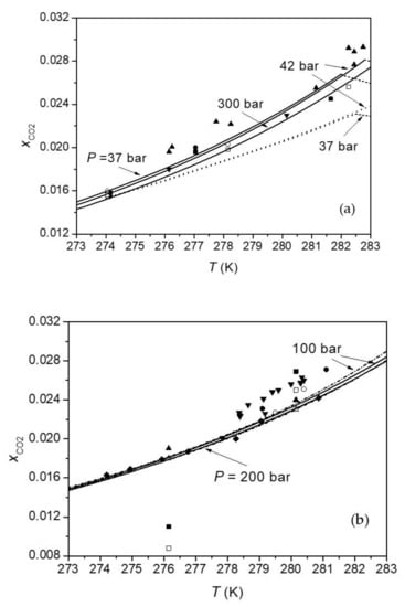
Figure 1.
Comparisons of predictions of this model for CO2 solubility in water at HLWE with experimental data. The solid and dash-dot lines are calculations of this model for CO2 solubility at HLWE with Method 1 and Method 2, respectively. The dotted lines are calculations of the model of Hashemi et al. [86] for HLWE. The dashed lines represent calculated CO2 solubility at vapor-liquid water equilibrium (VLWE). In 1 (a), symbols ■ and □ represent experimental data of Servio and Englezos [79] at 37 bar and 42 bar, symbols ● and ○ represent data of Sun et al. [84] at 37 bar and 42 bar, ▲ and ▼ represent data of Aya et al. [76] and Geng et al. [85] at 300 bar, respectively. In 1 (b), symbols ■ and □ represent experimental data of Lee et al. [78] at 100 bar and 200 bar, symbols ● and ○ represent data of Kim et al. [82] at 100 bar and 200 bar, ▲ and ∆ represent data of Geng et al. [85] at 100 bar and 200 bar, ▼ and ♦ represent data of Yang et al. [77] and Zhang et al. [83] at 100 bar, respectively.
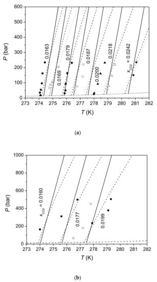
Figure 2.
Isopleths of CO2 solubility in water at HLWE. The solid and dash-dot lines are predictions of this model for CO2 solubility at HLWE with Method 1 and Method 2, respectively. The dotted lines are calculations of the model of Zhang et al. [83]. The dashed lines are calculated P-T lines of HLWV equilibrium. Symbols in 2 (a) represent experimental data of Zhang et al. [83] and symbols in 2 (b) represent experimental data of Zhang [80].
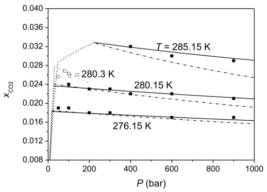
Figure 3.
Isotherms of CO2 solubility in water at HLWE. The solid and dash-dot lines are predictions of this model for CO2 solubility at HLWE with Method 1 and method 2, respectively. The dotted lines are calculations of the model of Yang et al. [77]. The dashed lines are CO2 solubility at VLWE or liquid CO2-liquid water equilibrium (LCLWE). Symbols ■ and □ represent experimental data of Geng et al. [85] and Yang et al. [77], respectively.
Figure 1a shows that CO2 solubility in water at HLWE increases with the increasing temperature whereas CO2 solubility at VLE decreases with the increasing temperature at constant pressure. The prediction of this model for the temperature dependence of CO2 solubility at HLWE is consistent with experimental data. As shown in Figure 2 and Figure 3, the pressure dependence of CO2 solubility at HLWE predicted by this model is negative, which is consistent with experimental data of Zhang [80], Zhang et al. [83], and Geng et al. [85]. It can also be seen from Figure 3 that the decreasing gradient of CO2 solubility with pressure at constant temperature is small. For example, CO2 solubility decreases by 10% when the pressure increases from 100 bar to 900 bar at 276.15 K according to the measurement of Geng et al. [85] and calculations of this model with Method 1. As mentioned before, Method 2 predicts larger pressure dependence of CO2 solubility than Method 1. Calculations of Method 1 are more consistent with data of Geng et al. [85] than Method 2, whereas calculations of Method 2 are more consistent with data of Zhang [80] than Method 1. Experimental data of Yang et al. [77], Servio and Englezos [79], and Kim et al. [82] show very weak pressure dependence of CO2 solubility at HLWE. Considering that the maximum pressure of these data is about 200 bar and the decrease of CO2 solubility within 200 bar is close to the uncertainty of experimental data, it is indeed difficult to find the change tendency of CO2 solubility with pressure from these data. On the other hand, experimental data measured by Zhang [80], Zhang et al. [83], and Geng et al. [85]), which cover a wider range of pressure than other experimental data, clearly show a negative pressure dependence of CO2 solubility at HLWE. Anyway, more measurements on CO2 solubility at HLWE are needed to verify this model.
Calculations of models of Hashemi et al. [86], Zhang et al. [83], and Yang et al. [77] were put into Figure 1, Figure 2, Figure 3, respectively. It can be seen that models of Zhang et al. [83] and Yang et al. [77] give a negative pressure dependence of CO2 solubility at HLWE, which is consistent with our model. In contrast, the model of Hashemi et al. [86] gives a positive pressure dependence of CO2 solubility at HLWE. The model of Yang et al. [77] gives a greater decrease gradient of CO2 solubility with increasing pressure than our model using Method 2, while the decrease gradient of CO2 solubility with increasing pressure predicted by the model of Zhang et al. [83] is comparable to that predicted by our model with Method 2. As shown in Figure 1, calculations of the model of Hashemi et al. [86] are lower than experimental data at 37 bar and 42 bar. Calculations of the model of Yang et al. [77] agree with experimental data reported in the same work, but are larger than those measured by other studies. The accuracy of the model of Zhang et al. [83] is comparable to our model since it adopted solubility models [101,113,114] which can accurately calculate CO2 solubility at vapor–liquid equilibrium. However, the model of Zhang et al. [83] overestimates the occupancy fraction of CO2 in small cage. Considering that composition of CO2 hydrate phase at HLWVE calculated by Sun and Duan [18] is accurate and the variation of composition of CO2 hydrate phase with pressure is small, we argue that calculations of this model for composition of CO2 hydrate phase at HLWE are reliable. However, experimental data on composition of hydrate phase at HLWE are needed for verifying our model. In general, this model is generally more accurate than previous models in CO2 solubility in aqueous solutions and in composition of hydrate phase. In addition, this model covers a larger range of pressure (up to 1000 bar) compared to previous models.
There are just a few experimental measurements of CO2 solubility in aqueous electrolyte solutions at HLWE, including measurements of CO2 solubility in aqueous NaCl solution made by Kim et al. [82] and Sun et al. [84], and measurement of CO2 solubility in artificial seawater made by Zhang et al. [83]. Unfortunately, there are some discrepancies among these data. Data reported by Kim et al. [82] show a salting-in effect for CO2 solubility at HLWE (in another word, CO2 solubility in NaCl solution is greater than that in pure water at the same temperature and pressure). In contrast, data measured by Zhang et al. [83] and Sun et al. [84] show a salting-out effect. The absolute average deviation of this model from experimental data of Kim et al. [82] and Sun et al. [84] are given in Table 3. Calculations of this model for CO2 solubility in aqueous NaCl solution at HLWE are lower than data of Kim et al. [82] because this model predicts a salting-out effect. Predictions of this model are consistent with experimental data of Sun et al. [84] in 1 wt% NaCl solution but are greater than their data in 3 wt% and 3.6 wt% NaCl solutions by 10–30%. Figure 4 shows that predictions of this model with Method 1 for CO2 solubility in artificial seawater agree well with data of Zhang et al. [83] (the AAD is 1.6%). Considering that the effect of 35‰ seawater on CO2 solubility is close to that of 3.6 wt% NaCl solution, the discrepancy between this model and data of Sun et al. [84] reflects the discrepancy between data of Zhang et al. [83] and Sun et al. [84].
Table 3.
The AAD of this model for CO2 solubility in aqueous NaCl solution at HLWE from experimental data sets.
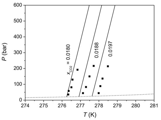
Figure 4.
Isopleths of CO2 solubility in 35‰ artificial water at HLWE. The solid lines are predictions of this model (with Method 1) for CO2 solubility at HLWE and the dashed lines are calculated P-T lines of HLWV equilibrium. Symbols represent experimental data of Zhang et al. [83].
For the effect of pressure on CO2 solubility in aqueous electrolyte solutions at HLWE, experimental data measured by Zhang et al. [83] and Sun et al. [84] show a negative trends whereas data of Kim et al. [82] show very weak pressure dependence. As shown in Figure 4, this model predicts that CO2 solubility in aqueous electrolyte solutions at HLWE decreases with the increasing pressure, similar to CO2 solubility in pure water. More measurements on CO2 solubility in aqueous NaCl solutions and in seawater at HLWE are needed to verify this model.
4. Conclusions
An accurate thermodynamic model was developed to predict CO2 solubility in pure water and in seawater at hydrate–liquid water equilibrium. The van der Waals–Platteeuw basic hydrate model was used to describe the chemical potential of hydrate phase. Angle-dependent ab initio intermolecular potentials were used to calculate the Langmuir constants of CO2 in hydrate cavities following our previous study. For the thermodynamic properties of the aqueous phase, two methods were adopted by this study. Method 1 is using the Pitzer model to calculate the activity of water and using the Poynting correction to calculate the fugacity of CO2 dissolved in water, and Method 2 is using the SAFT-LJ EOS to calculate the activity of water and the fugacity of dissolved CO2. No parameters of this model were evaluated from experimental data of HLWE so that calculations of this model for HLWE are predictive.
The comparison of calculations of this model with experimental data shows that this model can predict CO2 solubility in pure water and in seawater at HLWE with high accuracy. This model predicts that CO2 solubility at HLWE increases with increasing temperature, which agrees with available experimental measurements. This model predicts that CO2 solubility at HLWE decreases with increasing pressure and salinity. Most of the experimental data sets show negative pressure and salinity dependences of CO2 solubility at HLWE except one experimental data set showing a positive pressure dependence of CO2 solubility and one data set showing a positive salinity dependence of CO2 solubility. The predictions of this model for pressure and salinity dependences of CO2 solubility are consistent with most of experimental data. Two different methods to describe aqueous phase give similar change rate of CO2 solubility with temperature and salinity whereas Method 2 gives larger decrease of CO2 solubility with increasing pressure. This model covers a wider range of pressure (up to 1000 bar) than previous models and is generally more accurate than previous models in CO2 solubility in aqueous solutions and in composition of hydrate phase. Anyway, more measurements on CO2 solubility at HLWE are needed to verify this model. Extending our model to HLWE of CH4+CO2+N2 hydrate will be done in future. A computer program for the calculation of CO2 solubility in pure water and in seawater at hydrate–liquid water equilibrium can be obtained from the corresponding author via email.
Author Contributions
Conceptualization, R.S. and W.L.; methodology, R.S.; software, M.D. and R.S.; validation, M.D., L.G., and R.S.; formal analysis, M.D.; investigation, R.S. and L.G.; resources, R.S.; data curation, M.D. and L.G.; writing—original draft preparation, M.D. and R.S.; writing—review & editing, R.S.; visualization, M.D.; supervision, R.S. and W.L.; project administration, R.S. and W.L.; funding acquisition, R.S. All authors have read and agreed to the published version of the manuscript.
Funding
The work was funded by National Natural Science Foundation of China (Project 41773051 and 41373058), by MOST Special Fund from the State Key Laboratory of Continental Dynamics, Northwest University.
Data Availability Statement
There are no new data reported in this study and a computer program for the calculation of CO2 solubility in pure water and in seawater at hydrate–liquid water equilibrium can be obtained from the corresponding author via email.
Acknowledgments
The authors acknowledge three anonymous reviewers for their detailed, helpful, and pertinent comments which greatly improved the quality of the manuscript.
Conflicts of Interest
The authors declare no conflict of interest.
Abbreviations
| Nomenclature | |
| a | activity |
| Cij | the Langmuir constant of gas component j in i-type cavity |
| Cp | isobaric molar heat capacity (J/K/mol) |
| fj | the fugacity of gas component j (Pa) |
| h | molar enthalpy (J/mol) |
| kH | Henry’s law constant |
| P | pressure (Pa) |
| R | universal gas constant (= 8.314 J/mol/K) |
| T | temperature (K) |
| V | molar volume (m3/mol) |
| x | mole fraction |
| θij | the fractional occupancy of i-type cavities with j-type guest molecules |
| μ | molar chemical potential (J/mol) |
| νi | the number of i-type cages per water molecule |
| ρ | density (kg/m3) |
| partial molar volume (m3/mol) | |
| Subscript | |
| sol | solution |
| W | H2O |
| Superscript | |
| aq | aqueous phase |
| car | carbonic phase |
| H | hydrate phase |
| L | liquid water (aqueous phase) |
| sat | saturation |
| V | vapor phase |
| β | hypothetical empty hydrate lattice phase |
Appendix A
Appendix A.1. The Improved SAFT-LJ EOS
The SAFT-LJ EOS improved by Sun and Dubessy [55] is defined in terms of the dimensionless residual Helmholtz energy ares as follows:
where a represents the dimensionless molar Helmholtz energy, the superscript seg, chain, assoc, polar, and ion represent the contributions from the repulsive and the attractive forces between Lennard–Jones segments, the chain formation, the intermolecular association, the multi-polar interaction, and ion–ion interaction, respectively. The following are formula for every Helmholtz energy term.
Appendix A.2. Lennard–Jones Segment Term
The equation for aseg is
where mx is the segment number of mixtures, is the Helmholtz energy of one mole of non-associated spherical Lennard–Jones segments, and aHS is the molar Helmholtz energy of hard-sphere fluid. The Kolafa–Nezbeda equation [110] is used to calculate . All variables in Equation (A2) are calculated using the following equations:
where the subscript x means the variable for mixture, the superscript * means the reduced variable, kB is the Boltzmann constant, T is temperature in K, Vm is the molar volume in m3/mol, ρ is the density in mol/m3, η is the reduced packing density, m is the number of segments to form a non-spherical molecule, b is the molar volume of the segment, and ε is the Lennard–Jones energy parameter of the segment.
is the residual second virial coefficient, dBH is the ratio of the hard-sphere diameter to the soft-sphere diameter of the segment. Coefficients Ckl, γ, Ck, Dk, and Dln are component-independent, dimensionless, because they do not stand for any physical constants or variables. Their values were evaluated by Kolafa and Nezbeda [110] from computer simulation data for Lennard–Jones fluids. Parameters b, ε, and m are component-dependent. The value of the parameters b, ε, and m for pure CO2 and pure H2O are evaluated from the saturated vapor pressure and liquid density data. They are given in Table A1.
Table A1.
Parameters of SAFT-LJ EOS for pure H2O and pure CO2.
Table A1.
Parameters of SAFT-LJ EOS for pure H2O and pure CO2.
| H2O | CO2 | |
|---|---|---|
| ε/kB (K) | 172.1 − 0.001 × (T-473.15)2 | 173.7 |
| b (cm3/mol) | 16.684 − 0.00476 × (T-423.15) + 1.58 × 10⁻⁵ × (T-423.15)2 | 19.97 |
| εassoc/kB (K) | 1430 − 1.07 × (T-273.15) − 10.5 × 10⁻⁴ × (T-273.15)2 +7.5 × 10⁻⁶ × (T-273.15)3 | |
| Κassoc | 0.004 | |
| m | 1 | 1.5 |
| μ (10−30C·m) | 7.34 | |
| Q (10−40C·m2) | −14.3 |
For mixtures, the calculation of parameters mx, bx, and εx is based on van der Waals one-fluid mixing rule:
where xi is the mole fraction of component i. Parameters for the i-j interactions, bij and εij, are calculated by the following combining rules:
The dimensionless parameters k1,ij and k2,ij are empirical corrections of the Lorentz–Berthelot rules and they are fitted to vapor–liquid equilibria data of the binary system.
Appendix A.3. Chain-Forming Term
achain takes into account the change of Helmholtz energy due to the presence of covalent chain-forming bonds among the segments belonging to one molecule. Including the chain-forming term is also the distinct character of SAFT-type EOSs from other EOSs based on perturbation theories. In SAFT, achain is derived from Wertheim’s theory in the limit of a covalent bonding between the segments. The resulted expression is as follows:
where gLJ is the Lennard–Jones radial distribution function. and in Equation (A14) are defined as
Appendix A.4. Association Term
SAFT EOS adopts the thermodynamic perturbation theory of Wertheim [46,47,48] to calculate the Helmholtz energy contribution due to the intermolecular association (hydrogen-bonding force) as
where the sum runs over the species i and all the associating sites of species i, and Mi is the number of the associating sites of molecule i. XiA, the fraction of molecule i not bonded at site A, is obtained from the solution of the mass balance equation,
where NAv is Avogrado constant, is the associating strength between site A of species i and site B of species j. The improved SAFT-LJ EOS only takes into account the self-association among water molecules and ignored the cross-associations between H2O and CO2, between H2O and ion, and between ion and ion (It was assumed that NaCl is fully dissociated in aqueous solution below 573 K) so that Equation (A18) can be solved analytically. Because H2O is modeled as a spherical molecule with four association sites, can be calculated from the following equation:
Furthermore, Equation (A18) is simplified to
where the subscript w is the component H2O. The associating strength, Δ, depends on the radial distribution function and the interaction between two association sites. It is calculated using the following equation:
where bw is the volume of one mole water molecules (not molar volume of fluid phase) in m3/mol, parameters and are the association energy and association volume of water molecules, and are the reduced density and reduced temperature of water, respectively. The integral I is equal to 1.
Appendix A.5. Multi-Polar Term
The improved SAFT-LJ EOS considered the dipole moment of H2O and the quadrupole moment of CO2 but omit the quadrupole moment of H2O. The contribution of multi-polar interaction is calculated using the equation derived by Gubbins and Twu [111] based on the perturbation theory as follows:
The term contains three two-body terms and contains four two-body terms (a3A1, a3A2, a3A3, a3A4) and four three-body terms (a3B1, a3B2, a3B3, a3B4):
Detailed equations for a21, a22, a23, a3A1, … a3B4, can be found in Sun and Dubessy [54].
Appendix A.6. Charge–Charge Interaction Term
The restricted primitive model of mean spherical approximation [112] was adopted by the improved SAFT-LJ EOS to calculate aion. In the restricted primitive model of mean spherical approximation (MSA), the solvent is regarded as a continuous medium with specified dielectric constant D and different ions are modeled as charged hard spheres of equal diameter. The following is the equation for aion:
where d is the diameter of hydrated ion, and χ is a dimensionless quantity defined by
where κ is the Debye inverse screening length given by
In Equation (A29), ε0 is the vacuum permittivity, Dw is the dielectric constant of water, zj is the valence of the charged ion j, e is the charge of an electron, and the summation is over all ions in the mixture.
d is the sole adjustable parameter of Equation (A27). The short-range interaction Lennard–Jones parameters for Na+ and for Cl- are considered to be equal, i.e., bNa = bCl, and εNa = εCl. The parameters for the cross-interaction between ions and H2O are also assumed to be identical, i.e., bNa-H2O = bCl-H2O, and εNa-H2O = εCl-H2O. In the MSA theory, ions are assumed to be hard spheres and the dispersion force between ion and ion is not considered, thus εNa is equal to 0. bNa, bNa-H2O, εNa-H2O, and d were derived from the experimental data of the H2O-NaCl system and are listed in Table A2.
Table A2.
SAFT-LJ parameters for NaCl-H2O.
Table A2.
SAFT-LJ parameters for NaCl-H2O.
| Parameter | Value |
|---|---|
| d (10−10 m) | 4.65 + 0.00237 × (T-273.15) − 2.572 × 10⁻⁵ × (T-273.15)2 |
| εNaCl/kB (K) | 0 |
| bNaCl (cm3/mol) | 11.411 + 0.03052 × (T-273.15) − 2.389 × 10⁻⁴ × (T-273.15)2 + 3.048 × 10⁻⁷ × (T-273.15)3 |
| εNaCl-H2O/kB (K) | 283.01 − 0.0476 × (T-273.15) + 6.237 × 10⁻⁴ × (T-273.15)2 |
| bNaCl-H2O(cm3/mol) | 10.6 − 0.00521 × (T-273.15) − 6.3336 × 10⁻⁵ × (T-273.15)2 |
Similar to the cross-interaction parameters for ion-H2O, the values of the cross-interaction parameters for Na+-CO2 are equals to those of Cl--CO2, i.e., bNa-CO2 = bCl-CO2, and εNa-CO2 = εCl-CO2. This study assumes that εNa-CO2 = 0. Equation (A30) gives the temperature-dependent binary interaction parameter k2,ion-CO2 for the calculation of bNaCl-CO2.
References
- Bachu, S. Sequestration of CO2 in geological media: Criteria and approach for site selection in response to climate change. Energy Convers. Manag. 2000, 41, 953–970. [Google Scholar] [CrossRef]
- Cao, C.; Liu, H.; Hou, Z.; Mehmood, F.; Liao, J.; Feng, W. A review of CO2 storage in view of safety and cost-effectiveness. Energies 2020, 13, 600. [Google Scholar] [CrossRef]
- Adu, E.; Zhang, Y.; Liu, D. Current situation of carbon dioxide capture, storage, and enhanced oil recovery in the oil and gas industry. Can. J. Chem. Eng. 2019, 97, 1048–1076. [Google Scholar] [CrossRef]
- Leung, D.Y.; Caramanna, G.; Maroto-Valer, M.M. An overview of current status of carbon dioxide capture and storage technologies. Renew. Sustain. Energy Rev. 2014, 39, 426–443. [Google Scholar] [CrossRef]
- Brewer, P.G.; Friederich, G.; Peltzer, E.T.; Orr, F.M., Jr. Direct experiments on the ocean disposal of fossil fuel CO2. Science 1999, 284, 943–945. [Google Scholar] [CrossRef]
- De Silva, G.; Ranjith, P.; Perera, M. Geochemical aspects of CO2 sequestration in deep saline aquifers: A review. Fuel 2015, 155, 128–143. [Google Scholar] [CrossRef]
- Aminu, M.D.; Nabavi, S.A.; Rochelle, C.A.; Manovic, V. A review of developments in carbon dioxide storage. Appl. Energy 2017, 208, 1389–1419. [Google Scholar] [CrossRef]
- Blackford, J.; Alendal, G.; Avlesen, H.; Brereton, A.; Cazenave, P.W.; Chen, B.; Dewar, M.; Holt, J.; Phelps, J. Impact and detectability of hypothetical CCS offshore seep scenarios as an aid to storage assurance and risk assessment. Int. J. Greenh. Gas Control 2020, 95, 102949. [Google Scholar] [CrossRef]
- House, K.Z.; Schrag, D.P.; Harvey, C.F.; Lackner, K.S. Permanent carbon dioxide storage in deep-sea sediments. Proc. Natl. Acad. Sci. USA 2006, 103, 12291–12295. [Google Scholar] [CrossRef]
- Kvamme, B.; Graue, A.; Buanes, T.; Kuznetsova, T.; Ersland, G. Storage of CO2 in natural gas hydrate reservoirs and the effect of hydrate as an extra sealing in cold aquifers. Int. J. Greenh. Gas Control. 2007, 1, 236–246. [Google Scholar] [CrossRef]
- Tohidi, B.; Yang, J.; Salehabadi, M.; Anderson, R.; Chapoy, A. CO2 hydrates could provide secondary safety factor in subsurface sequestration of CO2. Environ. Sci. Technol. 2010, 44, 1509–1514. [Google Scholar] [CrossRef]
- Sun, D.; Englezos, P. Storage of CO2 in a partially water saturated porous medium at gas hydrate formation conditions. Int. J. Greenh. Gas Control. 2014, 25, 1–8. [Google Scholar] [CrossRef]
- Ohgaki, K.; Takano, K.; Sangawa, H.; Matsubara, T.; Nakano, S. Methane exploitation by carbon dioxide from gas hydrates. Phase equilibria for CO2-CH4 mixed hydrate system. J. Chem. Eng. Jpn. 1996, 29, 478–483. [Google Scholar] [CrossRef]
- Koh, D.-Y.; Kang, H.; Kim, D.-O.; Park, J.; Cha, M.; Lee, H. Recovery of methane from gas hydrates intercalated within natural sediments using CO2 and a CO2/N2 gas mixture. ChemSusChem 2012, 5, 1443–1448. [Google Scholar] [CrossRef]
- Belosludov, V.R.; Bozhko, Y.Y.; Subbotin, O.S.; Belosludov, R.V.; Zhdanov, R.K.; Gets, K.V.; Kawazoe, Y. Influence of N2 on formation conditions and guest distribution of mixed CO2 + CH4 gas hydrates. Molecules 2018, 23, 3336. [Google Scholar] [CrossRef]
- Zheng, J.; Chong, Z.R.; Qureshi, M.F.; Linga, P. Carbon dioxide sequestration via gas hydrates: A potential pathway toward decarbonization. Energy Fuels 2020, 34, 10529–10546. [Google Scholar] [CrossRef]
- Sloan, E.D.J.; Koh, C.A. Clathrate Hydrates of Natural Gases, 3rd ed.; CRC Press: Boca Raton, FL, USA, 2008. [Google Scholar]
- Sun, R.; Duan, Z. Prediction of CH4 and CO2 hydrate phase equilibrium and cage occupancy from ab initio intermolecular potentials. Geochim. Cosmochim. Acta 2005, 69, 4411–4424. [Google Scholar] [CrossRef]
- Van der Waals, J.H.; Platteeuw, J.C. Clathrate Solutions. In Advances in Chemical Physics; Prigogine, I., Ed.; Interscience: Geneva, Switzerland, 1959; pp. 1–57. [Google Scholar]
- Cao, Z.T.; Tester, J.W.; Sparks, K.A.; Trout, B.L. Molecular computations using robust hydrocarbon-water potentials for predicting gas hydrate phase equilibria. J. Phys. Chem. B 2001, 105, 10950–10960. [Google Scholar] [CrossRef]
- Klauda, J.B.; Sandler, S.I. Ab initio intermolecular potentials for gas hydrates and their predictions. J. Phys. Chem. B 2002, 106, 5722–5732. [Google Scholar] [CrossRef]
- Anderson, B.J.; Tester, J.W.; Trout, B.L. Accurate potentials for argon-water and methane-water interactions via ab initio methods and their application to clathrate hydrates. J. Phys. Chem. B 2004, 108, 18705–18715. [Google Scholar] [CrossRef]
- Lee, J.W.; Yedlapalli, P.; Lee, S. Prediction of hydrogen hydrate equilibrium by integrating ab initio calculations with statistical thermodynamics. J. Phys. Chem. B 2006, 110, 2332–2337. [Google Scholar] [CrossRef] [PubMed]
- Velaga, S.C.; Anderson, B.J. Carbon dioxide hydrate phase equilibrium and cage occupancy calculations using ab initio intermolecular potentials. J. Phys. Chem. B 2014, 118, 577–589. [Google Scholar] [CrossRef] [PubMed]
- Thakre, N.; Jana, A.K. Computing anisotropic cavity potential for clathrate hydrates. J. Phys. Chem. A 2019, 123, 2762–2770. [Google Scholar] [CrossRef]
- Veesam, S.K.; Ravipati, S.; Punnathanam, S.N. Recent advances in thermodynamics and nucleation of gas hydrates using molecular modeling. Curr. Opin. Chem. Eng. 2019, 23, 14–20. [Google Scholar] [CrossRef]
- Medeiros F de, A.; Segtovich, I.S.V.; Tavares, F.W.; Sum, A.K. Sixty years of the van der Waals and Platteeuw model for clathrate hydrates—A critical review from its statistical thermodynamic basis to its extensions and applications. Chem. Rev. 2020, 120, 13349–13381. [Google Scholar] [CrossRef]
- Thakre, N.; Jana, A.K. Physical and molecular insights to clathrate hydrate thermodynamics. Renew. Sustain. Energy Rev. 2021, 135, 110150. [Google Scholar] [CrossRef]
- Ballard, A.L.; Sloan, E.D. The next generation of hydrate prediction I: Hydrate standard states and incorporation of spectroscopy. Fluid Phase Equilibria 2002, 194−197, 371–383. [Google Scholar] [CrossRef]
- Klauda, J.B.; Sandler, S.I. Phase behavior of clathrate hydrates: A model for single and multiple gas component hydrates. Chem. Eng. Sci. 2003, 58, 27–41. [Google Scholar] [CrossRef]
- Belosludov, R.V.; Zhdanov, R.K.; Gets, K.V.; Bozhko, Y.Y.; Belosludov, V.R.; Kawazoe, Y. Role of methane as a second guest component in thermodynamic stability and isomer selectivity of butane clathrate hydrates. J. Phys. Chem. C 2020, 124, 18474–18481. [Google Scholar] [CrossRef]
- Kodera, M.; Matsueda, T.; Belosludov, R.V.; Zhdanov, R.K.; Belosludov, V.R.; Takeya, S.; Alavi, S.; Ohmura, R. Physical properties and characterization of the binary clathrate hydrate with methane + 1,1,1,3,3-pentafluoropropane (HFC-245fa) + water. J. Phys. Chem. C 2020, 124, 20736–20745. [Google Scholar] [CrossRef]
- Belosludov, V.R.; Subbotin, O.S.; Krupskii, D.S.; Belosludov, R.V.; Kawazoe, Y.; Kudoh, J.-I. Physical and chemical properties of gas hydrates: theoretical aspects of energy storage application. Mater. Trans. 2007, 48, 704–710. [Google Scholar] [CrossRef]
- Belosludov, R.V.; Subbotin, O.S.; Mizuseki, H.; Kawazoe, Y.; Belosludov, V.R. Accurate description of phase diagram of clathrate hydrates at the molecular level. J. Chem. Phys. 2009, 131, 244510. [Google Scholar] [CrossRef] [PubMed]
- Belosludov, R.V.; Bozhko, Y.Y.; Subbotin, O.S.; Belosludov, V.R.; Mizuseki, H.; Kawazoe, Y.; Fomin, V.M. Stability and composition of helium hydrates based on Ices I-h and II at low temperatures. J. Phys. Chem. C 2014, 118, 2587–2593. [Google Scholar] [CrossRef]
- Redlich, O.; Kwong, J.N.S. On the thermodynamics of solutions. V. An equation of state. Fugacities of gaseous solutions. Chem. Rev. 1949, 44, 233–244. [Google Scholar] [CrossRef] [PubMed]
- Peng, D.-Y.; Robinson, D.B. A new two-constant equation of state. Ind. Eng. Chem. Fundam. 1976, 15, 59–64. [Google Scholar] [CrossRef]
- Patel, N.C.; Teja, A.S. A new cubic equation of state for fluids and fluid mixtures. Chem. Eng. Sci. 1982, 37, 463–473. [Google Scholar] [CrossRef]
- Trebble, M.; Bishnoi, P. Development of a new four-parameter cubic equation of state. Fluid Phase Equilibria 1987, 35, 1–18. [Google Scholar] [CrossRef]
- Renon, H.; Prausnitz, J.M. Local compositions in thermodynamic excess functions for liquid mixtures. AIChE J. 1968, 14, 135–144. [Google Scholar] [CrossRef]
- Abrams, D.S.; Prausnitz, J.M. Statistical thermodynamics of liquid mixtures: A new expression for the excess Gibbs energy of partly or completely miscible systems. AIChE J. 1975, 21, 116–128. [Google Scholar] [CrossRef]
- Pitzer, K.S. (Ed.) Theory and data correlation. In Activity Coefficients in Electrolyte Solutions; CRC Press: London, UK, 1991; pp. 75–153. [Google Scholar]
- Esmaeilzadeh, F.; Hamedi, N.; Karimipourfard, D.; Rasoolzadeh, A. An insight into the role of the association equations of states in gas hydrate modeling: A review. Pet. Sci. 2020, 17, 1432–1450. [Google Scholar] [CrossRef]
- Chapman, W.G.; Gubbins, K.E.; Jackson, G.; Radosz, M. New reference equation of state for associating liquids. Ind. Eng. Chem. Res. 1990, 29, 1709–1721. [Google Scholar] [CrossRef]
- Huang, S.H.; Radosz, M. Equation of state for small, large, polydisperse, and associating molecules. Ind. Eng. Chem. Res. 1990, 29, 2284–2294. [Google Scholar] [CrossRef]
- Wertheim, M.S. Fluids with highly directional attractive forces: I. Statistical thermodynamics. J. Stat. Phys. 1984, 35, 19–34. [Google Scholar] [CrossRef]
- Wertheim, M.S. Fluids with highly directional attractive forces. II. Thermodynamic perturbation theory and integral equations. J. Stat. Phys. 1984, 35, 35–47. [Google Scholar] [CrossRef]
- Wertheim, M.S. Fluids with highly directional attractive forces: III. Multiple attraction sites. J. Stat. Phys. 1986, 42, 459–476. [Google Scholar] [CrossRef]
- Kontogeorgis, G.M.; Voutsas, E.C.; Yakoumis, I.V.; Tassios, D.P. An equation of state for associating fluids. Ind. Eng. Chem. Res. 1996, 35, 4310–4318. [Google Scholar] [CrossRef]
- Valtz, A.; Chapoy, A.; Coquelet, C.; Paricaud, P.; Richon, D. Vapor-liquid equilibria in the carbon dioxide-water system, measurement and modelling from 278.2 to 318.2K. Fluid Phase Equilibria 2004, 226, 333–344. [Google Scholar] [CrossRef]
- Ji, X.; Tan, S.P.; Adidharma, H.; Radosz, M. SAFT1-RPM approximation extended to phase equilibria and densities of CO2-H2O and CO2-H2O-NaCl systems. Ind. Eng. Chem. Res. 2005, 44, 8419–8427. [Google Scholar] [CrossRef]
- Dos Ramos, M.C.; Blas, F.J.; Galindo, A. Phase equilibria, excess properties, and Henry’s constants of the water + carbon dioxide binary mixture. J. Phys. Chem. C 2007, 111, 15924–15934. [Google Scholar] [CrossRef]
- Perfetti, E.; Thiery, R.; Dubessy, J. Equation of state taking into account dipolar interactions and association by hydrogen bonding: II: Modelling liquid-vapor equilibria in the H2O-H2S, H2O-CH4 and H2O-CO2 systems. Chem. Geol. 2008, 251, 50–57. [Google Scholar] [CrossRef]
- Sun, R.; Dubessy, J. Prediction of vapor–liquid equilibrium and PVTx properties of geological fluid system with SAFT-LJ EOS including multi-polar contribution. Part I. application to H2O–CO2 system. Geochim. Cosmochim. Acta 2010, 74, 1982–1998. [Google Scholar] [CrossRef]
- Sun, R.; Dubessy, J. Prediction of vapor-liquid equilibrium and PVTx properties of geological fluid system with SAFT-LJ EOS including multi-polar contribution. Part II. Application to H2O-NaCl and CO2-H2O-NaCl System. Geochim. Cosmochim. Acta 2012, 88, 130–145. [Google Scholar] [CrossRef]
- Niño-Amézquita, G.; Van Putten, D.; Enders, S. Phase equilibrium and interfacial properties of water + CO2 mixtures. Fluid Phase Equilibria 2012, 332, 40–47. [Google Scholar] [CrossRef]
- Islam, A.W.; Carlson, E.S. Application of SAFT equation for CO2 + H2O phase equilibrium calculations over a wide temperature and pressure range. Fluid Phase Equilibria 2012, 321, 17–24. [Google Scholar] [CrossRef]
- Courtial, X.; Ferrando, N.; de Hemptinne, J.-C.; Mougin, P. Electrolyte CPA equation of state for very high temperature and pressure reservoir and basin applications. Geochim. Cosmochim. Acta 2014, 142, 1–14. [Google Scholar] [CrossRef]
- Llovell, F.; Vega, L. Accurate modeling of supercritical CO2 for sustainable processes: Water+CO2 and CO2+fatty acid esters mixtures. J. Supercrit. Fluids 2015, 96, 86–95. [Google Scholar] [CrossRef]
- Jiang, H.; Panagiotopoulos, A.Z.; Economou, I.G. Modeling of CO2 solubility in single and mixed electrolyte solutions using statistical associating fluid theory. Geochim. Cosmochim. Acta 2016, 176, 185–197. [Google Scholar] [CrossRef]
- Chen, J.; Lu, J.; Li, Y. Equation of state SAFT-CP for vapour–liquid equilibria and mutual solubility of carbon dioxide and water. Mol. Phys. 2016, 114, 2451–2460. [Google Scholar] [CrossRef]
- Bian, X.-Q.; Xiong, W.; Kasthuriarachchi, D.T.K.; Liu, Y.-B. Phase equilibrium modeling for carbon dioxide solubility in aqueous sodium chloride solutions using an association equation of state. Ind. Eng. Chem. Res. 2019, 58, 10570–10578. [Google Scholar] [CrossRef]
- Sun, L.; Kontogeorgis, G.M.; Von Solms, N.; Liang, X. Modeling of gas solubility using the electrolyte cubic plus association equation of state. Ind. Eng. Chem. Res. 2019, 58, 17555–17567. [Google Scholar] [CrossRef]
- Chabab, S.; Théveneau, P.; Corvisier, J.; Coquelet, C.; Paricaud, P.; Houriez, C.; El Ahmar, E. Thermodynamic study of the CO2 – H2O – NaCl system: Measurements of CO2 solubility and modeling of phase equilibria using Soreide and Whitson, electrolyte CPA and SIT models. Int. J. Greenh. Gas Control. 2019, 91, 102825. [Google Scholar] [CrossRef]
- Pabsch, D.; Held, C.; Sadowski, G. Modeling the CO2 solubility in aqueous electrolyte solutions using ePC-SAFT. J. Chem. Eng. Data 2020, 65, 5768–5777. [Google Scholar] [CrossRef]
- Li, X.-S.; Wu, H.-J.; Englezos, P. Prediction of gas hydrate formation conditions in the presence of methanol, glycol, and triethylene glycol with statistical associating fluid theory equation of state. Ind. Eng. Chem. Res. 2006, 45, 2131–2137. [Google Scholar] [CrossRef]
- Li, X.-S.; Wu, H.-J.; Li, Y.-G.; Feng, Z.-P.; Tang, L.-G.; Fan, S.-S. Hydrate dissociation conditions for gas mixtures containing carbon dioxide, hydrogen, hydrogen sulfide, nitrogen, and hydrocarbons using SAFT. J. Chem. Thermodyn. 2007, 39, 417–425. [Google Scholar] [CrossRef]
- Haghighi, H.; Chapoy, A.; Tohidi, B. Methane and water phase equilibria in the presence of single and mixed electrolyte solutions using the cubic-plus-association equation of state. Oil Gas Sci. Technol. 2009, 64, 141–154. [Google Scholar] [CrossRef]
- Martín, Á.; Peters, C.J. New Thermodynamic model of equilibrium states of gas hydrates considering lattice distortion. J. Phys. Chem. C 2009, 113, 422–430. [Google Scholar] [CrossRef]
- Jiang, H.; Adidharma, H. Hydrate equilibrium modeling for pure alkanes and mixtures of alkanes using statistical associating fluid theory. Ind. Eng. Chem. Res. 2011, 50, 12815–12823. [Google Scholar] [CrossRef]
- Dufal, S.; Galindo, A.; Jackson, G.; Haslam, A.J. Modelling the effect of methanol, glycol inhibitors and electrolytes on the equilibrium stability of hydrates with the SAFT-VR approach. Mol. Phys. 2012, 110, 1223–1240. [Google Scholar] [CrossRef]
- Karakatsani, E.K.; Kontogeorgis, G.M. Thermodynamic modeling of natural gas systems containing water. Ind. Eng. Chem. Res. 2013, 52, 3499–3513. [Google Scholar] [CrossRef]
- Li, L.; Zhu, L.; Fan, J. The application of CPA-vdWP to the phase equilibrium modeling of methane-rich sour natural gas hydrates. Fluid Phase Equilibria 2016, 409, 291–300. [Google Scholar] [CrossRef]
- Meragawi, S.E.; Diamantonis, N.I.; Tsimpanogiannis, I.N.; Economou, I.G. Hydrate—Fluid phase equilibria modeling using PC-SAFT and Peng–Robinson equations of state. Fluid Phase Equilibria 2016, 413, 209–219. [Google Scholar] [CrossRef]
- Palma, A.M.; Queimada, A.J.; Coutinho, J.A.P. Modeling of hydrate dissociation curves with a modified cubic-plus-association equation of state. Ind. Eng. Chem. Res. 2019, 58, 14476–14487. [Google Scholar] [CrossRef]
- Aya, I.; Yamane, K.; Nariai, H. Solubility of CO2 and density of CO2 hydrate at 30 MPa. Energy 1997, 22, 263–271. [Google Scholar] [CrossRef]
- Yang, S.; Yang, I.; Kim, Y.; Lee, C. Measurement and prediction of phase equilibria for water+CO2 in hydrate forming conditions. Fluid Phase Equilibria 2000, 175, 75–89. [Google Scholar] [CrossRef]
- Lee, K.M.; Lee, H.; Lee, J.; Kang, J.M. CO2 hydrate behavior in the deep ocean sediments; phase equilibrium, formation kinetics, and solubility. Geophys. Res. Lett. 2002, 29, 2034. [Google Scholar] [CrossRef]
- Servio, P.; Englezos, P. Effect of temperature and pressure on the solubility of carbon dioxide in water in the presence of gas hydrate. Fluid Phase Equilibria 2001, 190, 127–134. [Google Scholar] [CrossRef]
- Zhang, Y. Formation of Hydrate from Single-Phase Aqueous Solutions. Master’s Thesis, University of Pittsburgh, Pittsburgh, PA, USA, 2003. [Google Scholar]
- Someya, S.; Bando, S.; Chen, B.; Song, Y.; Nishio, M. Measurement of CO2 solubility in pure water and the pressure effect on it in the presence of clathrate hydrate. Int. J. Heat Mass Transf. 2005, 48, 2503–2507. [Google Scholar] [CrossRef]
- Kim, Y.S.; Lim, B.D.; Lee, J.E.; Lee, C.S. Solubilities of carbon dioxide, methane, and ethane in sodium chloride solution containing gas hydrate. J. Chem. Eng. Data 2008, 53, 1351–1354. [Google Scholar] [CrossRef]
- Zhang, Y.; Holder, G.D.; Warzinski, R.P. Phase equilibrium in two-phase, water-rich-liquid, hydrate systems: Experiment and theory. Ind. Eng. Chem. Res. 2008, 47, 459–469. [Google Scholar] [CrossRef]
- Sun, Q.; Tian, H.; Li, Z.; Guo, X.; Liu, A.; Yang, L. Solubility of CO2 in water and NaCl solution in equilibrium with hydrate. Part I: Experimental measurement. Fluid Phase Equilibria 2016, 409, 131–135. [Google Scholar] [CrossRef]
- Geng, L.; Qu, K.; Lu, W.; Jiang, L.; Chou, I.-M. In situ Raman spectroscopic study of the pressure effect on the concentration of CO2 in water at hydrate-liquid water equilibrium up to 900 bar. Fluid Phase Equilibria 2017, 438, 37–43. [Google Scholar] [CrossRef]
- Hashemi, S.; Macchi, A.; Bergeron, S.; Servio, P. Prediction of methane and carbon dioxide solubility in water in the presence of hydrate. Fluid Phase Equilibria 2006, 246, 131–136. [Google Scholar] [CrossRef]
- Parrish, W.R.; Prausnitz, J.M. Dissociation pressures of gas hydrates formed by gas mixtures. Ind. Eng. Chem. Process. Des. Dev. 1972, 11, 26–35. [Google Scholar] [CrossRef]
- John, V.T.; Holder, G.D. Contribution of second and subsequent water shells to the potential energy of guest-host interactions in clathrate hydrates. J. Phys. Chem. 1982, 86, 455–459. [Google Scholar] [CrossRef]
- Zele, S.R.; Lee, S.-Y.; Holder, G.D. A theory of lattice distortion in gas hydrates. J. Phys. Chem. B 1999, 103, 10250–10257. [Google Scholar] [CrossRef]
- Lee, S.Y.; Holder, G.D. Model for gas hydrate equilibria using a variable reference chemical potential: Part 1. AICHE J. 2002, 48, 161–167. [Google Scholar] [CrossRef]
- Holder, G.; Zetts, S.; Pradhan, N. Phase behavior in systems containing clathrate hydrates: A review. Rev. Chem. Eng. 1988, 5, 1–70. [Google Scholar] [CrossRef]
- Sun, Q.; Tian, H.; Guo, X.; Liu, A.; Yang, L. Solubility of CO2 in water and NaCl solution in equilibrium with hydrate. Part II: Model calculation. Can. J. Chem. Eng. 2018, 96, 620–624. [Google Scholar] [CrossRef]
- Chen, G.-J.; Guo, T.-M. Thermodynamic modeling of hydrate formation based on new concepts. Fluid Phase Equilibria 1996, 122, 43–65. [Google Scholar] [CrossRef]
- Chen, G.-J.; Guo, T.-M. A new approach to gas hydrate modelling. Chem. Eng. J. 1998, 71, 145–151. [Google Scholar] [CrossRef]
- Bergeron, S.; Macchi, A.; Servio, P. Theoretical temperature dependency of gas hydrate former solubility under hydrate-liquid water equilibrium. J. Chem. Thermodyn. 2007, 39, 737–741. [Google Scholar] [CrossRef]
- Bergeron, S.; Beltrán, J.G.; Macchi, A.; Servio, P. Theoretical pressure dependency of carbon dioxide solubility under hydrate-liquid water equilibrium. Can. J. Chem. Eng. 2010, 88, 307–311. [Google Scholar] [CrossRef]
- Sun, R.; Duan, Z. An accurate model to predict the thermodynamic stability of methane hydrate and methane solubility in marine environments. Chem. Geol. 2007, 244, 248–262. [Google Scholar] [CrossRef]
- Holder, G.D.; Corbin, G.; Papadopoulos, K.D. Thermodynamic and molecular properties of gas hydrates from mixtures containing methane, argon, and krypton. Ind. Eng. Chem. Fundam. 1980, 19, 282–286. [Google Scholar] [CrossRef]
- Prausnitz, J.M.; Lichtenthaler, R.N.; Gomes de Azevedo, E. Molecular Thermodynamics of Fluid-Phase Equilibria; Prentice-Hall: Englewood Cliffs, NJ, USA, 1986. [Google Scholar]
- Holder, G.D.; Mokka, L.P.; Warzinski, R.P. Formation of gas hydrates from single-phase aqueous solutions. Chem. Eng. Sci. 2001, 56, 6897–6903. [Google Scholar] [CrossRef]
- Duan, Z.; Sun, R.; Zhu, C.; Chou, I.-M. An improved model for the calculation of CO2 solubility in aqueous solutions containing Na+, K+, Ca2+, Mg2+, Cl−, and SO42−. Mar. Chem. 2006, 98, 131–139. [Google Scholar] [CrossRef]
- Duan, Z.; Møller, N.; Weare, J.H. An equation of state for the CH4-CO2-H2O system: I. Pure systems from 0 to 1000 °C and 0 to 8000 bar. Geochim. Cosmochim. Acta 1992, 56, 2605–2617. [Google Scholar] [CrossRef]
- Dhima, A.; De Hemptinne, J.-C.; Jose, J. Solubility of hydrocarbons and CO2 mixtures in water under high pressure. Ind. Eng. Chem. Res. 1999, 38, 3144–3161. [Google Scholar] [CrossRef]
- Spencer, R.J.; Moller, N.; Weare, J.H. The prediction of mineral solubilities in natural waters: A chemical equilibrium model for the Na-K-Ca-Mg-Cl-SO4-H2O system at temperatures below 25 °C. Geochim. Cosmochim. Acta 1990, 54, 575–590. [Google Scholar] [CrossRef]
- Duan, Z.; Sun, R. A model to predict phase equilibrium of CH4 and CO2 clathrate hydrate in aqueous electrolyte solutions. Am. Miner. 2006, 91, 1346–1354. [Google Scholar] [CrossRef]
- Gil-Villegas, A.; Galindo, A.; Whitehead, P.J.; Mills, S.J.; Jackson, G.; Burgess, A.N. Statistical associating fluid theory for chain molecules with attractive potentials of variable range. J. Chem. Phys. 1997, 106, 4168–4186. [Google Scholar] [CrossRef]
- Adidharma, H.; Radosz, M. Prototype of an engineering equation of state for heterosegmented polymers. Ind. Eng. Chem. Res. 1998, 37, 4453–4462. [Google Scholar] [CrossRef]
- Gross, J.; Sadowski, G. Perturbed-Chain SAFT: An equation of state based on a perturbation theory for chain molecules. Ind. Eng. Chem. Res. 2001, 40, 1244–1260. [Google Scholar] [CrossRef]
- Kraska, T.; Gubbins, K.E. Phase equilibria calculations with a modified saft equation of state. 1. Pure Alkanes, Alkanols, and Water. Ind. Eng. Chem. Res. 1996, 35, 4727–4737. [Google Scholar] [CrossRef]
- Kolafa, J.; Nezbeda, I. The Lennard-Jones fluids. An accurate analytic and theoretically-based equation of state. Fluid Phase Equilibria 1994, 100, 1–34. [Google Scholar] [CrossRef]
- Twu, C.; Gubbins, K. Thermodynamics of polyatomic fluid mixtures—II. Chem. Eng. Sci. 1978, 33, 879–887. [Google Scholar] [CrossRef]
- Blum, L.; Hoeye, J.S. Mean spherical model for asymmetric electrolytes. 2. Thermodynamic properties and the pair correlation function. J. Phys. Chem. 1977, 81, 1311–1316. [Google Scholar] [CrossRef]
- Duan, Z.; Sun, R. An improved model calculating CO2 solubility in pure water and aqueous NaCl solutions from 273 to 533 K and from 0 to 2000 bar. Chem. Geol. 2003, 193, 257–271. [Google Scholar] [CrossRef]
- Diamond, L.W.; Akinfiev, N.N. Solubility of CO2 in water from −1.5 to 100 °C and from 0.1 to 100 MPa: evaluation of literature data and thermodynamic modelling. Fluid Phase Equilibria 2003, 208, 265–290. [Google Scholar] [CrossRef]
Publisher’s Note: MDPI stays neutral with regard to jurisdictional claims in published maps and institutional affiliations. |
© 2021 by the authors. Licensee MDPI, Basel, Switzerland. This article is an open access article distributed under the terms and conditions of the Creative Commons Attribution (CC BY) license (https://creativecommons.org/licenses/by/4.0/).