Least Absolute Deviation Estimation for Uncertain Regression Model via Uncertainty Distribution and Its Application in Sport Statistics

Abstract

Uncertain regression analysis is a powerful tool for analyzing and interpreting the complex relationships between explanatory and response variables under uncertain environments, and a crucial step in analyzing datasets containing complex uncertainties is statistical inference based on uncertain parameter estimation methods. However, the existing parameter estimation studies of uncertain regression models all fail to effectively avoid the negative impact of outliers on the estimation results. To solve the above problem and further enrich the parameter estimation research, this paper constructs a symmetric statistical invariant for the uncertain regression model based on observed data and uncertain disturbance terms. Based on this statistical invariant, the least absolute deviation criterion is applied to propose a least absolute deviation estimation for the uncertain regression model. Finally, two numerical examples are provided to illustrate the advantages of the proposed method compared to existing methods, and the comparative results show that in certain scenarios, the least absolute deviation estimation method exhibits superior performance compared to other existing methods in terms of mean squared error, mean absolute error, and mean absolute percentage error. Furthermore, as a byproduct of this paper, the proposed method is applied to sports statistics, and two empirical cases are also provided to demonstrate the effectiveness of this application.

1. Introduction

As a core method in statistics for exploring relationships between variables, the evolution of regression analysis reflects the continuous theoretical innovation and paradigm expansion within the discipline in order to address the ever-emerging challenges of real-world data. This evolution can be traced back to the revelation of Galton [1] for the “regression to the mean” law in genetic phenomena at the end of the 19th century, which laid the empirical foundation for the concept of regression. Subsequently, the classical linear regression analysis was established through the theoretical refinement of the least squares method, becoming the cornerstone of relationship modeling, and the classical discussions on this topic can be found in Draper and Smith [2].

As application scenarios have become increasingly complex, a series of key model variants have emerged. In order to handle categorical response variables, Berkson [3] systematically proposed a logistic regression model based on the Logit function. For the sake of overcoming estimation instability caused by multicollinearity of independent variables, Hoerl and Kennard [4] introduced ridge regression with L2 penalty. In the era of high-dimensional data analysis, to simultaneously perform variable selection and parameter estimation, Tibshirani [5] proposed lasso regression with L1 penalty. For the purpose of combining the advantages of ridge regression and lasso regression and handle highly correlated variable groups, Zou and Hastie [6] further developed elastic network regression.

Overall, regression analysis has evolved from a tool describing linear relationships into a vast methodological system encompassing parametric, nonparametric, and regularized methods, its development driven by a deep understanding and modeling need for complex data structures. For those wishing to gain a deep understanding of regression analysis methods and keep abreast of its latest developments, the following works are widely considered to be of significant reference value. The work of Freund et al. [7] systematically explained the principles of regression model construction, statistical inference, and diagnostic techniques, covering a variety of application scenarios from basic to advanced. The work of Sen and Srivastava [8] focused on the combination of theoretical framework and computational methods, providing readers with rigorous mathematical derivations and practical implementation guidance, and the work of Chatterjee and Simonoff [9] focused on the theoretical expansion and practical application of linear and generalized linear models, and explored contemporary hot topics such as high-dimensional data modeling. These documents not only comprehensively review the core concepts and application paradigms of regression analysis but also deeply analyze important recent advances in the field, such as regularization methods and nonparametric techniques, providing researchers with a crucial perspective on the evolution and cutting-edge trends of the discipline.

The aforementioned classic research methods are all based on probability theory, constructing nondeterministic phenomena arising from randomness in the real world into stochastic models with repeatability and statistical regularity, and characterizing them using mathematical tools such as probability distributions and random variables. However, in practical observation, besides the aforementioned stochastic environments, another fundamentally different type of uncertainty widely exists. Its core characteristic is that the related phenomena do not have a stable frequency of occurrence, or it is difficult to obtain reliable statistical regularities through a large number of repeated experiments. This type of uncertainty often stems from incomplete information, cognitive ambiguity, system complexity, or lack of knowledge, and its essence is closer to cognitive uncertainty than objective randomness. If we forcibly use probability theory tools to model a system with cognitive uncertainty, we will inevitably get a result of frequency instability, which will violate the original theoretical assumption (frequency stability assumption). Relevant references can be found in Jiang and Ye [10] and Liu [11]. Therefore, traditional probabilistic frameworks often face limitations in theoretical foundation or empirical evidence when dealing with such cognitive uncertainty or knowledge uncertainty problems. To rigorously characterize this cognitive uncertainty that cannot be fully described by the classical probability framework, Liu [12] and Liu [13] established and systematized a completely new axiomatic system of mathematics, named as uncertainty theory, which aims to provide a self-consistent quantitative and analytical tool for non-random phenomena that lack sufficient historical data, rely on expert beliefs, or have unique one-off occurrences. The regression analysis paradigm developed on this theoretical basis naturally gave rise to uncertain regression analysis, which was investigated by Yao and Liu [14]. This emerging branch replaces the random error term or parameters in traditional regression models with uncertain variables that follow the axiomatic system of uncertainty theory, thus constructing a new type of uncertain regression model.

Building upon the work of Yao and Liu [14], the uncertain regression model system has been systematically expanded and deepened. For example, addressing the modeling needs of multiple response variables, Ye and Liu [15] proposed a multiple uncertain regression model, achieving simultaneous analysis of the correlation structure between multidimensional variables. In addition, many scholars have also studied other types of uncertain regression models, such as uncertain regression models with autoregressive time series errors (Chen [16]) and moving average time series errors (Chen [17]), uncertain panel regression model (Jiang and Ye [10]), and uncertain nonparametric regression model (Ding and Zhang [18]). In addition to this, the statistical inference of unknown parameters and uncertain disturbance terms for uncertain regression models has always been a hot topic of academic attention. Among them, the research on statistical inference of unknown parameters has yielded rich results, with representative works including least squares estimation (Yao and Liu [14]), least absolute deviations estimation (Liu and Yang [19]), uncertain maximum likelihood estimation (Lio and Liu [20], and Liu and Qin [21]), Tukey’s biweight estimation (Chen [22]), and moment estimation (Liu [11]), while the exploration of statistical inference of uncertain disturbance terms has also accumulated a series of key research conclusions, and the relevant results includes moment estimation (Lio and Liu [23]), uncertain maximum likelihood estimation (Lio and Liu [20], and Liu and Liu [24]), and least squares estimation (Liu and Liu [25]).

However, the aforementioned parameter estimation studies of uncertain regression models all fail to effectively avoid the negative impact of outliers on the estimation results. In particular, the least squares estimation method based on the uncertainty distribution function suffers from this problem. Since the objective function is constructed based on the deviation between the empirical distribution function and the population distribution function, squaring actually increases the relative weight of the deviation caused by outliers in the objective function. To address this issue, this paper will apply the least absolute deviation criterion to construct the least absolute deviation estimation for uncertain regression model. The main contributions of this paper are as follows:

• A symmetric statistical invariant based on uncertain regression model was constructed, and the least absolute deviation estimation of the uncertain regression model was proposed by applying the least absolute deviation criterion to this statistical invariant.
• The least absolute deviation estimation of the uncertain regression model was applied to the uncertain linear regression model, uncertain exponential growth model, and uncertain logistic decay model, respectively, and the advantages of the proposed method were illustrated with two numerical examples.
• The method proposed in this paper was applied to two typical scenarios in sports statistics, and the corresponding uncertain statistical models were studied based on real data.

2. Estimating Unknown Parameters of Uncertainty Distribution via the Least Absolute Deviation Criterion

Determining the unknown parameters of the uncertainty distribution function is a fundamental step in constructing an uncertain statistical model. This process provides methodological support for subsequent statistical inference and decision-making, making it possible to achieve robust optimization and precise risk management of the system in an uncertain environment. Specifically, given a family of uncertainty distribution functions $\{{\Phi }_{\beta }:\beta \in \Theta \}$ with unknown parameters, where $\beta$ is the vector of unknown parameters to be determined and $\Theta$ is the parameters space. For an uncertain variable that follows this family of uncertainty distribution functions $\{{\Phi }_{\beta }:\beta \in \Theta \}$, we assume that a set of observed values data $x_1,x_2,\cdots ,x_n$ can be obtained through observations. Then the parameter estimation problem in uncertain statistics is determining the vector of unknown parameters $\beta$ in the family of uncertainty distribution functions $\{{\Phi }_{\beta }:\beta \in \Theta \}$ based on this set of observed values data and the operational rules of uncertainty theory.

One of the widely adopted fundamental ideas in the field of uncertain statistics is that by constructing a certain mathematical proximity measure, search for the optimal population distribution within the preset family of uncertainty distribution functions $\{{\Phi }_{\beta }:\beta \in \Theta \}$ such that the distance between this distribution function and the empirical distribution function derived from the observed values data $x_1,x_2,\cdots ,x_n$ is minimized, thereby determining the vector of unknown parameters $\beta$. Note that the empirical distribution function of the set of observed values data $x_1,x_2,\cdots ,x_n$ is

$$\sum _{i=1}^n{\displaystyle \frac{\mathbb{I}(x_i\in (-\infty ,x])}{n}}.$$

Based on this, Ning and Liu [26] constructed an objective function that estimates the vector of unknown parameters $\beta$ by minimizing the sum of the absolute values of the differences between the empirical distribution function of the set of observed values data and the assumed population distribution function ${\Phi }_{\beta }$. Specifically, the least absolute deviation estimation based on uncertainty distribution can be transformed into solving the following optimization problem,

$$\underset{\beta \in \Theta }{min}\sum _{i=1}^n\left|\sum _{j=1}^n{\displaystyle \frac{\mathbb{I}(x_j\in (-\infty ,x_i])}{n}}-{\Phi }_{\beta }\left(x_i\right)\right|.$$

(1)

To facilitate the subsequent construction of theoretical models and mathematical derivations, the parameter estimation based on the least squares criterion under the assumption of a normal uncertainty distribution will be presented below.

Assume that there is a set of independent and identically distributed observed values data $x_1,x_2,\cdots ,x_n$ follows a normal uncertainty distribution $\mathcal{N}(\mu ,\sigma )$, where $\mu$ is the expected value parameter and $\sigma >0$ is the standard deviation parameter. Note that the distribution function of the normal uncertainty distribution $\mathcal{N}(\mu ,\sigma )$ is

$${\Phi }_{\mu ,\sigma }={\displaystyle \frac{1}{{\displaystyle exp\left(\frac{\pi (\mu -x)}{\sqrt{3}\sigma }\right)+1}}}.$$

Then the least squares estimations of the unknown parameters $\mu$ and $\sigma$ are the solutions to the following optimization problem,

$$\underset{\mu ,\sigma >0}{min}\sum _{i=1}^n\left|\sum _{j=1}^n{\displaystyle \frac{\mathbb{I}(x_j\in (-\infty ,x_i])}{n}}-{\displaystyle \frac{1}{{\displaystyle exp\left(\frac{\pi (\mu -x_i)}{\sqrt{3}\sigma }\right)+1}}}\right|.$$

(2)

3. Symmetric Statistical Invariant of Uncertain Regression Model

In the standard setting of uncertain regression analysis, we usually assume the existence of p-dimensional explanatory variables $(x_1,x_2,\cdots ,x_p)$ and corresponding response variables y. To explore in depth the synergistic effect mechanism of these explanatory variables on the response variable under uncertain conditions, Yao and Liu [14] pioneered the construction of an uncertain regression model structure as follows,

$$y=f(x_1,x_2,\cdots ,x_p|\beta )+\epsilon .$$

(3)

The core innovation of this model lies in modeling the non-deterministic factors in the variable relationship that are difficult to quantify precisely as uncertain variables. Here, the function f represents the deterministic relationship structure between the explanatory variables $(x_1,x_2,\cdots ,x_p)$ and the response variable y, $\beta$ is the parameter vector to be estimated, and $\epsilon$ is defined as an uncertain disturbance term with zero expected value and standard deviation $\sigma$, denoted as $\mathcal{N}(0,\sigma )$.

Suppose that there is a set of observation sequences

$$(x_{i1},x_{i2},\cdots ,x_{ip},y_i)$$

with $i=1,2,\cdots ,n$ regarding the explanatory variables $(x_1,x_2,\cdots ,x_p)$ and the response variable y. If both the unknown parameter vector $\beta$ in the uncertain regression model (3) and the standard deviation $\sigma$ of the uncertain disturbance term $\epsilon$ take their theoretical true values, then based on the model structure, we can derive that

$$y-f(x_1,x_2,\cdots ,x_p|\beta )\sim \mathcal{N}(0,\sigma ).$$

After standardization transformation, the above formula becomes

$${\displaystyle \frac{y-f(x_1,x_2,\cdots ,x_p|\beta )}{\sigma }}\sim \mathcal{N}(0,1).$$

Substituting actual observed data $(x_{i1},x_{i2},\cdots ,x_{ip},y_i)$, $i=1,2,\cdots ,n$ into this expression, we can define a set of real-valued functions for the parameters $\beta$ and $\sigma$ as

$$h_i(\beta ,\sigma )={\displaystyle \frac{y_i-f(x_{i1},x_{i2},\cdots ,x_{ip}|\beta )}{\sigma }},i=1,2,\cdots ,n.$$

(4)

The above n functions $h_1(\beta ,\sigma ),h_2(\beta ,\sigma ),\cdots ,h_n(\beta ,\sigma )$ constructed in this way can be regarded as a set of concrete implementations of the standardized uncertain variables. According to the fundamental principles of uncertainty theory, this set of function values should follow a standard uncertain normal distribution $\mathcal{N}(0,1)$, that is, we can reasonably infer that

$$h_1(\beta ,\sigma ),h_2(\beta ,\sigma ),\cdots ,h_n(\beta ,\sigma )\sim \mathcal{N}(0,1)$$

(5)

when the unknown parameters $\beta$ and $\sigma$ take their theoretical true values. Thus, the problem of estimating the unknown parameters $\beta$ and $\sigma$ in the uncertain regression model (3) is transformed into finding the optimal parameter values such that $h_1(\beta ,\sigma ),h_2(\beta ,\sigma ),\cdots ,h_n(\beta ,\sigma )$ can be regarded as a set of observed values from the population distribution $\mathcal{N}(0,1)$ as much as possible. Here, the population distribution $\mathcal{N}(0,1)$ is the statistical invariant constructed in uncertain regression analysis, and then the corresponding parameter estimation problem in uncertain regression analysis is transformed into a parameter estimation problem based on this statistical invariant. Because the uncertainty distribution of the statistical invariant $\mathcal{N}(0,1)$ is symmetric about the zero point, it is also called the symmetric statistical invariant.

The following examples will present the symmetric statistical invariants of the specific uncertain regression models corresponding to observation sequences.

Example 1. 

Uncertain linear regression model is a classic and widely used statistical analysis method, whose core objective is to characterize the relationship between the response variable and one or more explanatory variables under uncertain environments through a linear function. Specifically, assuming we have a response variable y and p explanatory variables $x_1,x_2,\cdots ,x_p$, the uncertain linear regression model can be expressed as

$$y={\beta }_0+{\beta }_1{x}_1+{\beta }_2{x}_2+\cdots +{\beta }_p{x}_p+\epsilon ,$$

(6)

where ${\beta }_0$ is the intercept term, and ${\beta }_1,{\beta }_2,\cdots ,{\beta }_p$ are the regression coefficients corresponding to each independent variable, reflecting the marginal effect of each explanatory variable on the response variable, and the variable ε is the uncertain error term, which is usually assumed to follow a normal uncertainty distribution with zero mean and constant variance ${\sigma }^2$, in order to capture uncertain variations that the model cannot explain.

Suppose also that there is a set of observation sequences

$$(x_{i1},x_{i2},\cdots ,x_{ip},y_i)$$

(7)

with $i=1,2,\cdots ,n$ regarding the explanatory variables $(x_1,x_2,\cdots ,x_p)$ and the response variable y. Then it follows from (4) that the statistical invariants of uncertain linear regression model (6) corresponding to observation sequences (7) are

$$\begin{array}{cc}\hfill h_i({\beta }_0,{\beta }_1,\cdots ,{\beta }_p,\sigma )& ={\displaystyle \frac{y_i-{\beta }_0-{\beta }_1{x}_{i1}-{\beta }_2{x}_{i2}-\cdots -{\beta }_p{x}_{ip}}{\sigma }}\hfill \\ \hfill & ={\displaystyle \frac{{\displaystyle y_i-{\beta }_0-\sum _{l=1}^p{\beta }_l{x}_{il}}}{\sigma }},i=1,2,\cdots ,n.\hfill \end{array}$$

Example 2. 

Uncertain exponential growth model is a mathematical framework used to characterize the phenomenon where the growth rate is proportional to the current value under uncertain environments, characterized by slow initial growth followed by rapid acceleration. This dynamic process is commonly seen in biological population growth, financial investment appreciation, and diffusion processes. Specifically, assuming we have a response variable y and a explanatory variable x, the uncertain exponential growth model can be expressed as

$$y={\beta }_0+{\beta }_{1}exp\left({\beta }_{2}x\right)+\epsilon ,{\beta }_1>0,{\beta }_2>0,$$

(8)

where ${\beta }_0$ denotes the initial reference level or lower limit, ${\beta }_1$ represents the initial size or scaling factor when $x=0$, while ${\beta }_2$ is the growth rate parameter, which determines the speed of process expansion, and the variable ε is the uncertain error term, which is usually assumed to follow a normal uncertainty distribution with zero mean and constant variance ${\sigma }^2$, in order to capture uncertain variations that the model cannot explain.

Suppose also that there is a set of observation sequences

$$(x_i,y_i)$$

(9)

with $i=1,2,\cdots ,n$ regarding the explanatory variable x and the response variable y. Then it follows from (4) that the statistical invariants of uncertain exponential growth model (8) corresponding to observation sequences (9) are

$$\begin{array}{cc}\hfill h_i({\beta }_0,{\beta }_1,{\beta }_2,\sigma )& ={\displaystyle \frac{y_i-{\beta }_0-{\beta }_{1}exp\left({\beta }_2{x}_i\right)}{\sigma }},i=1,2,\cdots ,n.\hfill \end{array}$$

Example 3. 

Uncertain logistic decay model is a mathematical model used to describe the dynamic characteristics of the decay process under uncertain environments, which typically unfolds in three stages: initial decay with slow acceleration, a significant increase in the decay rate in the middle stage, and a gradual leveling off in the later stage. This S-shaped decay curve is commonly seen in natural and social phenomena such as biodegradation processes, chemical decomposition, and increasing market saturation. Specifically, assuming we have a response variable y and a explanatory variable x, the uncertain logistic decay model can be expressed as

$$y={\beta }_0+{\displaystyle \frac{{\beta }_1}{1+{\beta }_{2}exp\left({\beta }_{3}x\right)}}+\epsilon ,$$

(10)

where ${\beta }_0$ denotes the initial reference level, ${\beta }_1$ represents the initial value or maximum possible value of the decay process, ${\beta }_2$ controls the horizontal position of the curve, while ${\beta }_3$ determines the decay rate, and the variable ε is the uncertain error term, which is usually assumed to follow a normal uncertainty distribution with zero mean and constant variance ${\sigma }^2$, in order to capture uncertain variations that the model cannot explain.

Suppose also that there is a set of observation sequences

$$(x_i,y_i)$$

(11)

with $i=1,2,\cdots ,n$ regarding the explanatory variable x and the response variable y. Then it follows from (4) that the statistical invariants of uncertain exponential growth model (10) corresponding to observation sequences (11) are

$$\begin{array}{cc}\hfill h_i({\beta }_0,{\beta }_1,{\beta }_2,{\beta }_3,\sigma )& ={\displaystyle \frac{{\displaystyle y_i-{\beta }_0-\frac{{\beta }_1}{1+{\beta }_{2}exp\left({\beta }_3{x}_i\right)}}}{\sigma }},i=1,2,\cdots ,n.\hfill \end{array}$$

4. Least Absolute Deviation Estimation of Uncertain Regression Model

This section will systematically study the parameter estimation problem in uncertain regression analysis based on the least absolute deviation criterion, focusing on how to determine the least absolute deviation estimation of the unknown parameter vector and disturbance term in the model within the framework of uncertainty theory, and thus establish a new parameter estimation method in uncertain regression analysis.

Based on the above analysis, the least absolute deviation problem of the unknown parameters and the uncertain disturbance term in the uncertain regression model (3) is transformed into the least absolute deviation estimation problem of the uncertainty distribution function with $h_1(\beta ,\sigma ),h_2(\beta ,\sigma ),\cdots ,h_n(\beta ,\sigma )$ as the observed values data and $\mathcal{N}(0,1)$ as the population distribution.

It should be noted that the empirical distribution function constructed from the function values $h_1(\beta ,\sigma ),h_2(\beta ,\sigma ),\cdots ,h_n(\beta ,\sigma )$ can be expressed as

$$\sum _{i=1}^n{\displaystyle \frac{\mathbb{I}(h_i(\beta ,\sigma )\in (-\infty ,x])}{n}}.$$

Moreover, the theoretical distribution function of the standard normal uncertainty distribution $\mathcal{N}(0,1)$ has the following analytical form,

$${\displaystyle \frac{1}{exp\left({\displaystyle \frac{-\pi x}{\sqrt{3}}}\right)+1}}.$$

Then based on the basic criterion of least absolute deviation estimation and optimization problem (1), the estimated values of parameters $\beta$ and $\sigma$ can be obtained by solving the following optimization problem,

$$\underset{\beta ,\sigma >0}{min}\sum _{i=1}^n\left|\sum _{j=1}^n{\displaystyle \frac{\mathbb{I}(h_j(\beta ,\sigma )\in (-\infty ,h_i(\beta ,\sigma )])}{n}}-{\displaystyle \frac{1}{exp\left({\displaystyle \frac{-\pi h_i(\beta ,\sigma )}{\sqrt{3}}}\right)+1}}\right|.$$

(12)

Here the solutions $\widehat{\beta }$ and $\widehat{\sigma }$ to the optimization problem (12) is also referred to as the least absolute deviation estimation of the uncertain regression model (3).

The following examples will present the least absolute deviation estimations of the specific uncertain regression models.

Example 4. 

According to optimization problem (12), the least absolute deviation estimations of ${\beta }_0,{\beta }_1,\cdots ,{\beta }_p$ and σ in Example 1 solve the following optimization problem

$$\begin{array}{cc}\hfill \underset{{\beta }_0,{\beta }_1,\cdots ,{\beta }_p,\sigma >0}{min}& \sum _{i=1}^n\left|\sum _{j=1}^n{\displaystyle \frac{\mathbb{I}\left({\displaystyle y_j-\sum _{l=1}^p{\beta }_l{x}_{jl}\le y_i-\sum _{l=1}^p{\beta }_l{x}_{il}}\right)}{n}}\right.\hfill \\ \hfill & \left.-{\left(exp\left({\displaystyle \frac{-\pi \left({\displaystyle y_i-{\beta }_0-\sum _{l=1}^p{\beta }_l{x}_{il}}\right)}{\sqrt{3}\sigma }}\right)+1\right)}^{-1}\right|.\hfill \end{array}$$

(13)

Example 5. 

According to optimization problem (12), the least absolute deviation estimations of ${\beta }_0,{\beta }_1,{\beta }_2$ and σ in Example 2 solve the following optimization problem

$$\begin{array}{cc}\hfill \underset{{\beta }_0,{\beta }_1,{\beta }_2,\sigma >0}{min}& \sum _{i=1}^n\left|\sum _{j=1}^n{\displaystyle \frac{\mathbb{I}\left(y_j-{\beta }_{1}exp\left({\beta }_2{x}_j\right)\le y_i-{\beta }_{1}exp\left({\beta }_2{x}_i\right)\right)}{n}}\right.\hfill \\ \hfill & \left.-{\left(exp\left({\displaystyle \frac{-\pi \left(y_i-{\beta }_0-{\beta }_{1}exp\left({\beta }_2{x}_i\right)\right)}{\sqrt{3}\sigma }}\right)+1\right)}^{-1}\right|.\hfill \end{array}$$

(14)

Example 6. 

According to optimization problem (12), the least absolute deviation estimations of ${\beta }_0,{\beta }_1,{\beta }_2,{\beta }_3$ and σ in Example 3 solve the following optimization problem

$$\begin{array}{cc}\hfill \underset{{\beta }_0,{\beta }_1,{\beta }_2,{\beta }_3,\sigma >0}{min}& \sum _{i=1}^n\left|\sum _{j=1}^n{\displaystyle \frac{\mathbb{I}\left({\displaystyle y_j-\frac{{\beta }_1}{1+{\beta }_{2}exp\left({\beta }_3{x}_j\right)}\le y_i-\frac{{\beta }_1}{1+{\beta }_{2}exp\left({\beta }_3{x}_i\right)}}\right)}{n}}\right.\hfill \\ \hfill & \left.-{\left(exp\left({\displaystyle \frac{-\pi \left({\displaystyle y_i-{\beta }_0-\frac{{\beta }_1}{1+{\beta }_{2}exp\left({\beta }_3{x}_i\right)}}\right)}{\sqrt{3}\sigma }}\right)+1\right)}^{-1}\right|.\hfill \end{array}$$

(15)

5. Numerical Examples

In this section, we will provide two numerical examples to illustrate the method of least absolute deviation estimation of the specific uncertain regression model, and compare it with existing methods to demonstrate the effectiveness of the method proposed in this paper.

Example 7. 

Consider an uncertain exponential growth model, mathematically expressed as

$$\begin{array}{c}\hfill y={\beta }_0+{\beta }_{1}exp\left({\beta }_{2}x\right)+\epsilon .\end{array}$$

(16)

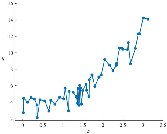
In this model, ${\beta }_0$, ${\beta }_1>0$, and ${\beta }_2>0$ are parameters to be estimated, and ε is an uncertain disturbance term, assumed to follow a normal uncertainty distribution with an expected value of 0 and a standard deviation of σ. For empirical analysis, we consider a dataset containing 50 sets of observations, presented in Table 1 and Figure 1, reflecting the observed relationship between the independent variable x and the response variable y.

Table 1. Dataset containing 50 sets of observations of uncertain exponential growth model (16) in Example 7.

x	y	x	y	x	y	x	y
0.0163	2.7465	1.0188	4.4031	1.5788	6.1850	2.4138	10.5860
0.0225	4.4697	1.0588	5.6984	1.5913	5.4555	2.4750	10.5586
0.1200	4.0093	1.1413	2.9662	1.6525	4.6591	2.4975	10.4439
0.2088	4.5790	1.1550	5.3076	1.6600	6.7465	2.6100	10.4084
0.2863	4.3957	1.2588	5.2089	1.7263	7.3172	2.6288	11.2445
0.3538	3.6632	1.3300	4.6746	1.7950	5.9218	2.6863	8.6729
0.3575	2.1197	1.3638	3.8767	1.9000	7.0619	2.8063	10.5416
0.4288	4.3062	1.3750	5.6668	1.9575	7.3112	2.8800	12.3008
0.5488	4.1479	1.4025	3.6343	2.0400	9.2094	2.9113	12.3081
0.6525	2.9091	1.4188	6.0522	2.1625	8.5153	3.0075	14.2273
0.7013	4.2475	1.4413	5.7321	2.2525	7.8449	3.1225	14.0800
0.8025	3.7803	1.4600	3.7853	2.3338	8.4899
0.9175	4.6032	1.4950	5.4228	2.3388	8.7107

Figure 1. Dataset containing 50 sets of observations of uncertain exponential growth model (16) in Example 7.

Denote the dataset by $(x_i,y_i)$ with $i=1,2,\cdots ,50$. Then it follows from Example 2 that the statistical invariants of uncertain exponential growth model (16) corresponding to dataset $(x_i,y_i)$, $i=1,2,\cdots ,50$ are

$$\begin{array}{cc}\hfill h_i({\beta }_0,{\beta }_1,{\beta }_2,\sigma )& ={\displaystyle \frac{y_i-{\beta }_0-{\beta }_{1}exp\left({\beta }_2{x}_i\right)}{\sigma }},i=1,2,\cdots ,50.\hfill \end{array}$$

By using the conclusion of Example 5, we can infer that the least absolute deviation estimations of ${\beta }_0,{\beta }_1,{\beta }_2$ and σ are the optimal solutions of the following optimization problem,

$$\begin{array}{cc}\hfill \underset{{\beta }_0,{\beta }_1,{\beta }_2,\sigma >0}{min}& \sum _{i=1}^{50}\left|\sum _{j=1}^{50}{\displaystyle \frac{\mathbb{I}\left(y_j-{\beta }_{1}exp\left({\beta }_2{x}_j\right)\le y_i-{\beta }_{1}exp\left({\beta }_2{x}_i\right)\right)}{50}}\right.\hfill \\ \hfill & \left.-{\left(exp\left({\displaystyle \frac{-\pi \left(y_i-{\beta }_0-{\beta }_{1}exp\left({\beta }_2{x}_i\right)\right)}{\sqrt{3}\sigma }}\right)+1\right)}^{-1}\right|,\hfill \end{array}$$

which can be obtained as

$${\widehat{\beta }}_0=1.9804,{\widehat{\beta }}_1=1.0734,{\widehat{\beta }}_2=0.8018,\widehat{\sigma }=1.0131.$$

Based on this, a fitted uncertain exponential growth model can be obtained as

$$y=1.9804+1.0734exp\left(0.8018x\right)+\mathcal{N}(0,1.0131).$$

(17)

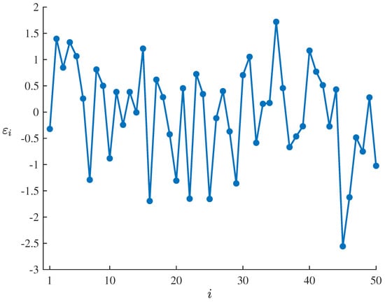
To test the suitability of the fitted uncertain exponential growth model (17) for the dataset $(x_i,y_i)$, $i=1,2,\cdots ,50$, the residuals of the estimated model corresponding to the dataset can be calculated by means of

$${\epsilon }_i=y_i-{\widehat{\beta }}_0-{\widehat{\beta }}_{1}exp\left({\widehat{\beta }}_2{x}_i\right),i=1,2,\cdots ,50,$$

which are showed in Table 2 and Figure 2. Set the significance level as $\alpha =0.05$, it follows from the uncertain hypothesis testing proposed by Ye and Liu [27] that the corresponding standardized critical value is

$$\pm {\displaystyle \frac{\sqrt{3}\widehat{\sigma }}{\pi }}log{\displaystyle \frac{\alpha }{2-\alpha }}=\pm 2.0464,$$

and the test is

$$\begin{array}{cc}\hfill W=\{({\epsilon }_1,{\epsilon }_2,\cdots ,{\epsilon }_{50}):& \mathrm{there} \mathrm{are} \mathrm{at} \mathrm{least} 3 \mathrm{of} \mathrm{indexes} i^{\prime }\mathrm{s} \mathrm{with} 1\le i\le 50\hfill \\ \hfill & \mathrm{such} \mathrm{that} {\epsilon }_i<-2.0464 \mathrm{or} {\epsilon }_i>2.0464\}.\hfill \end{array}$$

As shown in Table 2 and Figure 2, only ${\epsilon }_{45}$ is outside the interval $[-2.0464,2.0464]$, which does not meet the condition that the number of outliers with $|{\epsilon }_i|>2.0464$ is at least 3. Thus

$$({\epsilon }_1,{\epsilon }_2,\cdots ,{\epsilon }_{50})\notin W,$$

therefore failing to reject the compatibility assumption of the estimated model at significance level of $\alpha =0.05$. This result indicates that the fitted uncertain exponential growth model (17) can well adapt to and fit the dataset $(x_i,y_i)$, $i=1,2,\cdots ,50$.

Table 2. Residuals of the fitted uncertain exponential growth model (17) corresponding to the dataset $(x_i,y_i)$, $i=1,2,\cdots ,50$.

−0.3214	1.3963	0.8470	1.3297	1.0650	0.2574	−1.2905	0.8120
0.5008	−0.8825	0.3836	−0.2429	0.3828	−0.0068	1.2094	−1.6944
0.6173	0.2835	−0.4238	−1.3073	0.4537	−1.6508	0.7238	0.3427
−1.6558	−0.1167	0.3983	−0.3695	−1.3595	0.7036	1.0526	−0.5855
0.1569	0.1739	1.7195	0.4568	−0.6684	−0.4632	−0.2704	1.1710
0.7694	0.5125	−0.2734	0.4309	−2.5576	−1.6231	−0.4842	−0.7511
0.2794	−1.0238

Figure 2. Residuals of the fitted uncertain exponential growth model (17) corresponding to the dataset $(x_i,y_i)$, $i=1,2,\cdots ,50$.

Finally, based on the dataset $(x_i,y_i)$, $i=1,2,\cdots ,50$ in Table 1 and Figure 1, we will combine the existing parameter estimation methods for uncertain regression models, such as the least squares estimation method studied by Wang et al. [28] and the uncertain maximum likelihood estimation method explored by Liu and Qin [21], to perform statistical inference on the uncertain exponential growth model (16), and obtain

$$y=0.1011+2.0153exp\left(0.6578x\right)+\mathcal{N}(0,1.3340)$$

(18)

estimated based on the least squares estimation method and

$$y=2.1632+0.8277exp\left(0.8822x\right)+\mathcal{N}(0,1.0456)$$

(19)

estimated based on the uncertain maximum likelihood estimation method, respectively. To further compare the performance of the models, the mean squared error (MSE), mean absolute error (MAE), and mean absolute percentage error (MAPE) of models (17)–(19) on the same dataset $(x_i,y_i)$, $i=1,2,\cdots ,50$ are calculated, and the corresponding calculation formulas are as follows,

$$\mathrm{MSE}={\displaystyle \frac{1}{50}}\sum _{i=1}^{50}{\left({\widehat{\beta }}_0+{\widehat{\beta }}_{1}exp\left({\widehat{\beta }}_2{x}_i\right)-y_i\right)}^2,$$

$$\mathrm{MAE}={\displaystyle \frac{1}{50}}\sum _{i=1}^{50}|{\widehat{\beta }}_0+{\widehat{\beta }}_{1}exp\left({\widehat{\beta }}_2{x}_i\right)-y_i|$$

and

$$\mathrm{MAPE}={\displaystyle \frac{1}{50}}\sum _{i=1}^{50}\left|{\displaystyle \frac{{\widehat{\beta }}_0+{\widehat{\beta }}_{1}exp\left({\widehat{\beta }}_2{x}_i\right)-y_i}{y_i}}\right|,$$

respectively. Table 3 lists the comparison results of the error indices for these three estimated models. The result in the Table 3 shows that the MSE, MAE and MAPE obtained based on model (17) are all lower than those corresponding to models (18) and (19). This difference indicates that the least absolute deviation estimation method proposed in this paper exhibits superior fitting and prediction performance in parameter estimation of uncertain regression models.

Table 3. The MSEs, MAEs and MAPEs of estimated uncertain exponential growth models (17)–(19).

Methods	MSE	MAE	MAPE
least absolute deviation estimation method proposed in this paper	0.8818	0.7690	0.1485
least squares estimation method studied by Wang et al. [28]	1.3923	0.9570	0.1778
uncertain maximum likelihood estimation method explored by Liu and Qin [21]	0.9237	0.8047	0.1505

Example 8. 

Consider an uncertain logistic decay model, mathematically expressed as

$$\begin{array}{c}\hfill y={\beta }_0+{\displaystyle \frac{{\beta }_1}{1+{\beta }_{2}exp\left({\beta }_{3}x\right)}}+\epsilon .\end{array}$$

(20)

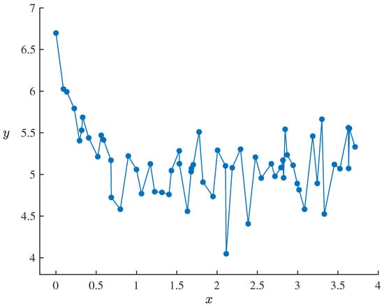
In this model, ${\beta }_0$, ${\beta }_1$, ${\beta }_2$, and ${\beta }_3$ are parameters to be estimated, and ε is an uncertain disturbance term, assumed to follow a normal uncertainty distribution with an expected value of 0 and a standard deviation of σ. For empirical analysis, we consider a dataset containing 60 sets of observations, presented in Table 4 and Figure 3, reflecting the observed relationship between the independent variable x and the response variable y.

Table 4. Dataset containing 60 sets of observations of uncertain logistic decay model (20) in Example 8.

x	y	x	y	x	y	x	y
0.0013	6.6980	1.0625	4.7696	2.1050	5.1033	3.0175	4.8159
0.0938	6.0260	1.1725	5.1271	2.1138	4.0478	3.0863	4.5819
0.1350	5.9927	1.2263	4.7929	2.1888	5.0805	3.1875	5.4604
0.2275	5.7929	1.3163	4.7848	2.2913	5.3033	3.2438	4.8927
0.2938	5.4052	1.4038	4.7598	2.3863	4.4076	3.3013	5.6636
0.3200	5.5313	1.4338	5.0465	2.4763	5.2073	3.3313	4.5252
0.3325	5.6864	1.5313	5.2841	2.5488	4.9567	3.4563	5.1203
0.4075	5.4392	1.5325	5.1293	2.6738	5.1283	3.5250	5.0693
0.5200	5.2136	1.6325	4.5580	2.7188	4.9779	3.6300	5.5617
0.5625	5.4709	1.6788	5.0340	2.7938	5.0824	3.6325	5.0722
0.5913	5.4155	1.6825	5.0730	2.8175	5.1713	3.6425	5.5523
0.6838	5.1706	1.7050	5.1167	2.8263	4.9600	3.7125	5.3314
0.6875	4.7240	1.7775	5.5110	2.8450	5.5425
0.8000	4.5824	1.8250	4.9078	2.8700	5.2348
0.8988	5.2218	1.9500	4.7352	2.9438	5.1105
1.0000	5.0596	2.0063	5.2905	2.9950	4.8911

Figure 3. Dataset containing 60 sets of observations of uncertain logistic decay model (20) in Example 8.

Denote the dataset by $(x_i,y_i)$ with $i=1,2,\cdots ,60$. Then it follows from Example 3 that the statistical invariants of uncertain logistic decay model (20) corresponding to dataset $(x_i,y_i)$, $i=1,2,\cdots ,60$ are

$$\begin{array}{cc}\hfill h_i({\beta }_0,{\beta }_1,{\beta }_2,{\beta }_3,\sigma )& ={\displaystyle \frac{{\displaystyle y_i-{\beta }_0-\frac{{\beta }_1}{1+{\beta }_{2}exp\left({\beta }_3{x}_i\right)}}}{\sigma }},i=1,2,\cdots ,60.\hfill \end{array}$$

By using the conclusion of Example 6, we can infer that the least absolute deviation estimations of ${\beta }_0,{\beta }_1,{\beta }_2,{\beta }_3$ and σ are the optimal solutions of the following optimization problem,

$$\begin{array}{cc}\hfill \underset{{\beta }_0,{\beta }_1,{\beta }_2,{\beta }_3,\sigma >0}{min}& \sum _{i=1}^{60}\left|\sum _{j=1}^{60}{\displaystyle \frac{\mathbb{I}\left({\displaystyle y_j-\frac{{\beta }_1}{1+{\beta }_{2}exp\left({\beta }_3{x}_j\right)}\le y_i-\frac{{\beta }_1}{1+{\beta }_{2}exp\left({\beta }_3{x}_i\right)}}\right)}{60}}\right.\hfill \\ \hfill & \left.-{\left(exp\left({\displaystyle \frac{-\pi \left({\displaystyle y_i-{\beta }_0-\frac{{\beta }_1}{1+{\beta }_{2}exp\left({\beta }_3{x}_i\right)}}\right)}{\sqrt{3}\sigma }}\right)+1\right)}^{-1}\right|,\hfill \end{array}$$

which can be obtained as

$${\hat{\beta }}_0=5.1207,{\widehat{\beta }}_1=-0.0218,{\widehat{\beta }}_2=-2.4583,{\widehat{\beta }}_3=32.6027,\widehat{\sigma }=0.3794.$$

Based on this, a fitted uncertain logistic decay model can be obtained as

$$y=5.1207+{\displaystyle \frac{-0.0218}{1-2.4583exp\left(32.6027x\right)}}+\mathcal{N}(0,0.3794)$$

(21)

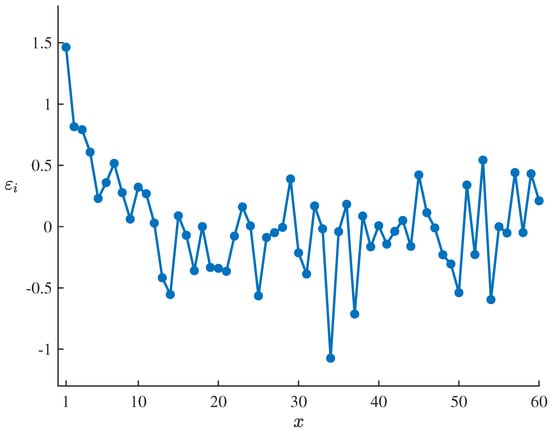
To test the suitability of the fitted uncertain logistic decay model (21) for the dataset $(x_i,y_i)$, $i=1,2,\cdots ,60$, the residuals of the estimated model corresponding to the dataset can be calculated by means of

$${\epsilon }_i=y_i-{\widehat{\beta }}_0-{\displaystyle \frac{{\widehat{\beta }}_1}{1+{\widehat{\beta }}_{2}exp\left({\widehat{\beta }}_3{x}_i\right)}},i=1,2,\cdots ,60,$$

which are showed in Table 5 and Figure 4. Set the significance level as $\alpha =0.1$, it follows from the uncertain hypothesis testing proposed by Ye and Liu [27] that the corresponding standardized critical value is

$$\pm {\displaystyle \frac{\sqrt{3}\widehat{\sigma }}{\pi }}log{\displaystyle \frac{\alpha }{2-\alpha }}=\pm 0.6159,$$

and the test is

$$\begin{array}{cc}\hfill W=\{({\epsilon }_1,{\epsilon }_2,\cdots ,{\epsilon }_{60}):& \mathrm{there} \mathrm{are} \mathrm{at} \mathrm{least} 7 \mathrm{of} \mathrm{indexes} i^{\prime } \mathrm{s}\mathrm{with}1\le i\le 60\hfill \\ \hfill & \mathrm{such} \mathrm{that} {\epsilon }_i<-0.6159 \mathrm{or} {\epsilon }_i>0.6159\}.\hfill \end{array}$$

As shown in Table 5 and Figure 4, only ${\epsilon }_1,{\epsilon }_2,{\epsilon }_3,{\epsilon }_{34},{\epsilon }_{37}$ are outside the interval $[-0.6159,0.6159]$, which does not meet the condition that the number of outliers with $|{\epsilon }_i|>0.6159$ is at least 7. Thus

$$({\epsilon }_1,{\epsilon }_2,\cdots ,{\epsilon }_{60})\notin W,$$

therefore failing to reject the compatibility assumption of the estimated model at significance level of $\alpha =0.1$. This result indicates that the fitted uncertain logistic decay model (21) can well adapt to and fit the dataset $(x_i,y_i)$, $i=1,2,\cdots ,60$.

Table 5. Residuals of the fitted uncertain logistic decay model (21) corresponding to the dataset $(x_i,y_i)$, $i=1,2,\cdots ,60$.

1.4637	0.8153	0.7908	0.6077	0.2298	0.3593	0.5161	0.2773
0.0617	0.3221	0.2686	0.0291	−0.4173	−0.5539	0.0888	−0.0706
−0.3593	0.0002	−0.3333	−0.3402	−0.3644	−0.0775	0.1609	0.0061
−0.5647	−0.0885	−0.0494	−0.0056	0.3889	−0.2141	−0.3864	0.1690
−0.0180	−1.0735	−0.0406	0.1823	−0.7133	0.0864	−0.1642	0.0075
−0.1429	−0.0384	0.0506	−0.1607	0.4218	0.1140	−0.0103	−0.2296
−0.3049	−0.5388	0.3397	−0.2280	0.5429	−0.5955	−0.0004	−0.0514
0.4410	−0.0485	0.4316	0.2107

Figure 4. Residuals of the fitted uncertain logistic decay model (21) corresponding to the dataset $(x_i,y_i)$, $i=1,2,\cdots ,60$.

Finally, based on the dataset $(x_i,y_i)$, $i=1,2,\cdots ,60$ in Table 4 and Figure 3, we will combine the existing parameter estimation methods for uncertain regression models, such as the least squares estimation method studied by Wang et al. [28] and the uncertain maximum likelihood estimation method explored by Liu and Qin [21], to perform statistical inference on the uncertain exponential growth model (16), and obtain

$$y=99.1773+{\displaystyle \frac{24.9373}{1-0.1450exp(-32.9138x)}}+\mathcal{N}(0,1.0417)$$

(22)

estimated based on the least squares estimation method and

$$y=4.9204+{\displaystyle \frac{17.5329}{1+-156.3587exp(-11.2862x)}}+\mathcal{N}(0,7.6665)$$

(23)

estimated based on the uncertain maximum likelihood estimation method, respectively. To further compare the performance of the models, the mean squared error (MSE), mean absolute error (MAE), and mean absolute percentage error (MAPE) of models (21)–(23) on the same dataset $(x_i,y_i)$, $i=1,2,\cdots ,60$ are calculated, and the corresponding calculation formulas are as follows,

$$\mathrm{MSE}={\displaystyle \frac{1}{60}}\sum _{i=1}^{60}{\left({\widehat{\beta }}_0+{\displaystyle \frac{{\widehat{\beta }}_1}{1+{\widehat{\beta }}_{2}exp\left({\widehat{\beta }}_3{x}_i\right)}}-y_i\right)}^2,$$

$$\mathrm{MAE}={\displaystyle \frac{1}{60}}\sum _{i=1}^{60}\left|{\widehat{\beta }}_0+{\displaystyle \frac{{\widehat{\beta }}_1}{1+{\widehat{\beta }}_{2}exp\left({\widehat{\beta }}_3{x}_i\right)}}-y_i\right|$$

and

$$\mathrm{MAPE}={\displaystyle \frac{1}{60}}\sum _{i=1}^{60}\left|{\displaystyle \frac{{\displaystyle {\widehat{\beta }}_0+\frac{{\widehat{\beta }}_1}{1+{\widehat{\beta }}_{2}exp\left({\widehat{\beta }}_3{x}_i\right)}-y_i}}{y_i}}\right|,$$

respectively. Table 6 lists the comparison results of the error indices for these three estimated models. The result in the Table 6 shows that the MSE, MAE and MAPE obtained based on model (21) are all lower than those corresponding to models (22) and (23). This difference indicates that the least absolute deviation estimation method proposed in this paper exhibits superior fitting and prediction performance in parameter estimation of uncertain regression models.

Table 6. The MSEs, MAEs and MAPEs of estimated uncertain logistic decay models (21)–(23).

Methods	MSE	MAE	MAPE
least absolute deviation estimation method proposed in this paper	0.1647	0.2928	0.0568
least squares estimation method studied by Wang et al. [28]	0.9454	0.7718	0.1467
uncertain maximum likelihood estimation method explored by Liu and Qin [21]	0.8576	0.4413	0.0798

6. Application in Sport Statistics

In sports statistics, scientifically quantifying the complex relationship between athletes’ physiological indicators, athletic performance, and economic value is crucial for training optimization, talent selection, and market evaluation. However, sports data is often affected by measurement errors, individual differences, and outliers. Traditional regression methods are sensitive to outliers, potentially weakening the model’s robustness and explanatory power. Therefore, this section introduces uncertain regression model and least absolute deviation criterion method to improve the stability and reliability of statistical inference under non-ideal data environments in sports statistics.

Specifically, this section focuses on two typical sports statistics scenarios: First, modeling the correlation between athletes’ physiological indicators and athletic performance. We select the weight, speed and agility performance, and flexibility and strength performance of adolescent athletes as explanatory variables to explore their relationship with lung capacity. In this scenario, individual physiological compensation and fluctuations in test conditions can easily lead to observational anomalies. Uncertain regression models and least absolute deviation criterion can effectively suppress the interference of outliers on model parameters, revealing the intrinsic correlations more robustly. Second, predicting the market value of FIFA football players. Player market value is influenced by multiple uncertain variables, including age, overall rating, international reputation, weak foot, skill moves, and often includes a few high-leverage observed values (such as superstar players). Traditional regression methods are easily affected by extreme values, leading to systematic biases in prediction. This section constructs an uncertain regression model based on the least absolute deviation criterion to enhance the inclusiveness of unconventional observed values and improve the robustness and practical reference value of market value prediction. Through empirical analysis of the two scenarios described above, this section systematically verifies the advantages of least absolute deviation estimation in sports statistics, providing a more robust and stable analytical method for modeling complex sports data, and promoting the cross-integration of statistical methods and sports science.

6.1. Uncertain Lung Capacity Model

To investigate the relationship between weight, speed and agility performance, flexibility and strength performance and lung capacity of young athletes, Li [29] collected relevant data from 18 young athletes, as shown in Table 7.

Table 7. Dataset of the weight, speed and agility performance, flexibility and strength performance and lung capacity of 18 young athletes.

Lung Capacity (mL)	Weight (kg)	Speed and Agility Performance (s)	Flexibility and Strength Performance (cm)
1905	58	9	11
1940	60	11	12
1975	62	12	14
2080	64	13	18
2045	66	13	15
2115	70	14	20
2185	72	15	23
2220	76	15	24
2255	78	16	25
2270	80	17	25
2300	83	19	30
2290	84	20	28
1875	56	7	9
2150	72	14	21
2285	82	18	24
2025	64	12	15
1800	52	5	6
1835	54	5	7

Let the lung capacity of the adolescent athletes be the response variable y, and let the weight ($x_1$), speed and agility performance ($x_2$), and flexibility and strength performance ($x_3$) of the adolescent athletes be the explanatory variables. And represent the dataset in Table 7 as

$$(y_i,x_{i1},x_{i2},x_{i3}),i=1,2,\cdots ,18.$$

Then we use the following uncertain linear regression model,

$$\begin{array}{c}\hfill y={\beta }_0+{\beta }_1{x}_1+{\beta }_2{x}_2+{\beta }_3{x}_3+\epsilon ,\end{array}$$

(24)

to fit the dataset $(y_i,x_{i1},x_{i2},x_{i3})$, $i=1,2,\cdots ,18$. In this model, ${\beta }_0$, ${\beta }_1$, ${\beta }_2$, and ${\beta }_3$ are parameters to be estimated, and $\epsilon$ is an uncertain disturbance term, assumed to follow a normal uncertainty distribution with an expected value of 0 and a standard deviation of $\sigma$.

It follows from Example 1 that the statistical invariants of uncertain linear regression model (24) corresponding to dataset $(y_i,x_{i1},x_{i2},x_{i3})$, $i=1,2,\cdots ,18$ are

$$\begin{array}{cc}\hfill h_i({\beta }_0,{\beta }_1,{\beta }_2,{\beta }_3,\sigma )& ={\displaystyle \frac{y_i-{\beta }_0-{\beta }_1{x}_1-{\beta }_2{x}_2-{\beta }_3{x}_3}{\sigma }},i=1,2,\cdots ,18.\hfill \end{array}$$

By using the conclusion of Example 4, we can infer that the least absolute deviation estimations of ${\beta }_0,{\beta }_1,{\beta }_2,{\beta }_3$ and $\sigma$ are the optimal solutions of the following optimization problem,

$$\begin{array}{cc}\hfill \underset{{\beta }_0,{\beta }_1,{\beta }_2,{\beta }_3,\sigma >0}{min}& \sum _{i=1}^{18}\left|\sum _{j=1}^{18}{\displaystyle \frac{\mathbb{I}\left({\displaystyle y_j-\sum _{l=1}^3{\beta }_l{x}_{jl}\le y_i-\sum _{l=1}^3{\beta }_l{x}_{il}}\right)}{18}}\right.\hfill \\ \hfill & \left.-{\left(exp\left({\displaystyle \frac{-\pi \left({\displaystyle y_i-{\beta }_0-\sum _{l=1}^3{\beta }_l{x}_{il}}\right)}{\sqrt{3}\sigma }}\right)+1\right)}^{-1}\right|,\hfill \end{array}$$

which can be obtained as

$${\widehat{\beta }}_0=1472.9510,{\widehat{\beta }}_1=5.3044,{\widehat{\beta }}_2=-5.5439,{\widehat{\beta }}_3=17.5744,\widehat{\sigma }=25.4603.$$

Based on this, a fitted uncertain lung capacity model can be obtained as

$$y=1472.9510+5.3044x_1-5.5439x_2+17.5744x_3+\mathcal{N}(0,25.4603).$$

(25)

To test the suitability of the fitted uncertain lung capacity model (25) for the dataset $(y_i,x_{i1},x_{i2},x_{i3})$, $i=1,2,\cdots ,18$, the residuals of the estimated model corresponding to the dataset can be calculated by means of

$${\epsilon }_i=y_i-{\widehat{\beta }}_0-{\widehat{\beta }}_1{x}_{i1}-{\widehat{\beta }}_2{x}_{i2}-{\widehat{\beta }}_3{x}_{i3},i=1,2,\cdots ,18,$$

which are showed in Table 8 and Figure 5. Set the significance level as $\alpha =0.1$, it follows from the uncertain hypothesis testing proposed by Ye and Liu [27] that the corresponding standardized critical value is

$$\pm {\displaystyle \frac{\sqrt{3}\widehat{\sigma }}{\pi }}log{\displaystyle \frac{\alpha }{2-\alpha }}=\pm 41.3310,$$

and the test is

$$\begin{array}{cc}\hfill W=\{({\epsilon }_1,{\epsilon }_2,\cdots ,{\epsilon }_{18}):& \mathrm{there} \mathrm{are} \mathrm{at} \mathrm{least} 2 \mathrm{of} \mathrm{indexes} i^{\prime }\mathrm{s} \mathrm{with} 1\le i\le 18\hfill \\ \hfill & \mathrm{such} \mathrm{that} {\epsilon }_i<-41.3310 \mathrm{or} {\epsilon }_i>41.3310\}.\hfill \end{array}$$

As shown in Table 8 and Figure 5, only ${\epsilon }_{15}$ is outside the interval $[-41.3310,41.3310]$, which does not meet the condition that the number of outliers with $|{\epsilon }_i|>41.3310$ is at least 2. Thus

$$({\epsilon }_1,{\epsilon }_2,\cdots ,{\epsilon }_{18})\notin W,$$

therefore failing to reject the compatibility assumption of the estimated model at significance level of $\alpha =0.1$. This result indicates that the fitted uncertain lung capacity model (25) can well adapt to and fit the dataset $(y_i,x_{i1},x_{i2},x_{i3})$, $i=1,2,\cdots ,18$.

Table 8. Residuals of the fitted uncertain lung capacity model (25) corresponding to the dataset $(y_i,x_{i1},x_{i2},x_{i3})$, $i=1,2,\cdots ,18$.

−19.0317	−1.1272	−6.3411	23.2962	30.4106	−3.1354	9.0763	5.2841
17.6447	27.5797	−35.1180	−9.7297	−14.3617	3.6813	55.0892	15.4756
−26.5084	−19.6917

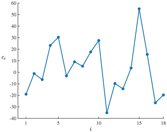
Figure 5. Residuals of the fitted uncertain lung capacity model (25) corresponding to the dataset $(y_i,x_{i1},x_{i2},x_{i3})$, $i=1,2,\cdots ,18$.

6.2. Uncertain FIFA Football Player Valuation Model

To investigate the relationship between age, overall rating, international reputation, weak foot, skill moves and the player market value, we collected relevant data from 28 football players retrieved from Website [30], as shown in Table 9.

Table 9. Dataset of the age, overall rating, international reputation, weak foot, skill moves and the player market value of 28 football players.

Market Value (Million)	Age	Overall Rating	International Reputation	Weak Foot	Skill Moves
83	29	92	5	4	4
37.5	28	86	3	3	3
41.5	29	87	4	4	3
41.5	24	86	4	4	3
71.5	23	88	4	4	5
72	26	90	4	3	4
20.5	25	82	3	3	3
14.5	31	83	3	3	3
54	30	89	4	4	4
87	31	94	5	4	5
35	30	86	3	4	4
4.8	34	81	3	3	3
31.5	27	86	3	3	3
12.5	33	84	4	3	3
18.5	29	82	3	4	3
29.5	26	84	2	4	4
15.5	23	80	3	3	3
24	26	83	2	3	3
30	28	86	4	4	4
20	21	81	2	4	3
23.5	21	81	1	3	3
5.5	27	77	2	2	3
18	33	84	4	4	3
14	30	82	2	1	3
20	26	82	2	3	3
11.5	31	80	2	3	2
10	30	80	2	3	2
19	28	82	3	2	4

Let the player market value of the football players be the response variable y, and let the age ($x_1$), overall rating ($x_2$), international reputation ($x_3$), weak foot ($x_4$), and skill moves ($x_5$) of the football playerss be the explanatory variables. And represent the dataset in Table 9 as

$$(y_i,x_{i1},x_{i2},x_{i3},x_{i4},x_{i5}),i=1,2,\cdots ,28.$$

Then we use the following uncertain linear regression model,

$$\begin{array}{c}\hfill y={\beta }_0+{\beta }_1{x}_1+{\beta }_2{x}_2+{\beta }_3{x}_3+{\beta }_4{x}_4+{\beta }_5{x}_5+\epsilon ,\end{array}$$

(26)

to fit the dataset $(y_i,x_{i1},x_{i2},x_{i3},x_{i4},x_{i5})$, $i=1,2,\cdots ,28$. In this model, ${\beta }_0$, ${\beta }_1$, ${\beta }_2$, ${\beta }_3$, ${\beta }_4$, and ${\beta }_5$ are parameters to be estimated, and $\epsilon$ is an uncertain disturbance term, assumed to follow a normal uncertainty distribution with an expected value of 0 and a standard deviation of $\sigma$.

It follows from Example 1 that the statistical invariants of uncertain linear regression model (26) corresponding to dataset $(y_i,x_{i1},x_{i2},x_{i3},x_{i4},x_{i5})$, $i=1,2,\cdots ,28$ are

$$\begin{array}{cc}\hfill h_i({\beta }_0,{\beta }_1,{\beta }_2,{\beta }_3,{\beta }_4,{\beta }_5,\sigma )& ={\displaystyle \frac{y_i-{\beta }_0-{\beta }_1{x}_1-{\beta }_2{x}_2-{\beta }_3{x}_3-{\beta }_4{x}_4-{\beta }_5{x}_5}{\sigma }}\hfill \end{array}$$

with $i=1,2,\cdots ,28$. By using the conclusion of Example 4, we can infer that the least absolute deviation estimations of ${\beta }_0,{\beta }_1,{\beta }_2,{\beta }_3,{\beta }_4,{\beta }_5$ and $\sigma$ are the optimal solutions of the following optimization problem,

$$\begin{array}{cc}\hfill \underset{{\beta }_0,{\beta }_1,{\beta }_2,{\beta }_3,{\beta }_4,{\beta }_5,\sigma >0}{min}& \sum _{i=1}^{28}\left|\sum _{j=1}^{28}{\displaystyle \frac{\mathbb{I}\left({\displaystyle y_j-\sum _{l=1}^5{\beta }_l{x}_{jl}\le y_i-\sum _{l=1}^5{\beta }_l{x}_{il}}\right)}{28}}\right.\hfill \\ \hfill & \left.-{\left(exp\left({\displaystyle \frac{-\pi \left({\displaystyle y_i-{\beta }_0-\sum _{l=1}^5{\beta }_l{x}_{il}}\right)}{\sqrt{3}\sigma }}\right)+1\right)}^{-1}\right|,\hfill \end{array}$$

which can be obtained as

$${\widehat{\beta }}_0=-380.3405,{\widehat{\beta }}_1=-0.7326,{\widehat{\beta }}_2=5.0971,{\widehat{\beta }}_3=-0.0499,{\widehat{\beta }}_4=-1.7853,{\widehat{\beta }}_5=2.3416,$$

and

$$\widehat{\sigma }=7.4316.$$

Based on this, a fitted uncertain FIFA football player valuation model can be obtained as

$$y=-380.3405-0.7326x_1+5.0971x_2-0.0499x_3-1.7853x_4+2.3416x_5+\mathcal{N}(0,7.4316).$$

(27)

To test the suitability of the fitted uncertain FIFA football player valuation model (27) for the dataset $(y_i,x_{i1},x_{i2},x_{i3},x_{i4},x_{i5})$, $i=1,2,\cdots ,28$, the residuals of the estimated model corresponding to the dataset can be calculated by means of

$${\epsilon }_i=y_i-{\widehat{\beta }}_0-{\widehat{\beta }}_1{x}_{i1}-{\widehat{\beta }}_2{x}_{i2}-{\widehat{\beta }}_3{x}_{i3}-{\widehat{\beta }}_4{x}_{i4}-{\widehat{\beta }}_5{x}_{i5},i=1,2,\cdots ,28,$$

which are showed in Table 10 and Figure 6. Set the significance level as $\alpha =0.05$, it follows from the uncertain hypothesis testing proposed by Ye and Liu [27] that the corresponding standardized critical value is

$$\pm {\displaystyle \frac{\sqrt{3}\widehat{\sigma }}{\pi }}log{\displaystyle \frac{\alpha }{2-\alpha }}=\pm 15.0106,$$

and the test is

$$\begin{array}{cc}\hfill W=\{({\epsilon }_1,{\epsilon }_2,\cdots ,{\epsilon }_{28}):& \mathrm{there} \mathrm{are} \mathrm{at} \mathrm{least} 2 \mathrm{of} \mathrm{indexes} i^{\prime }\mathrm{s} \mathrm{with} 1\le i\le 28\hfill \\ \hfill & \mathrm{such} \mathrm{that} {\epsilon }_i<-15.0106 \mathrm{or} {\epsilon }_i>15.0106\}.\hfill \end{array}$$

As shown in Table 10 and Figure 6, only ${\epsilon }_5$ is outside the interval $[-15.0106,15.0106]$, which does not meet the condition that the number of outliers with $|{\epsilon }_i|>15.0106$ is at least 2. Thus

$$({\epsilon }_1,{\epsilon }_2,\cdots ,{\epsilon }_{28})\notin W,$$

therefore failing to reject the compatibility assumption of the estimated model at significance level of $\alpha =0.05$. This result indicates that the fitted uncertain FIFA football player valuation model (27) can well adapt to and fit the dataset $(y_i,x_{i1},x_{i2},x_{i3},x_{i4},x_{i5})$, $i=1,2,\cdots ,28$.

Table 10. Residuals of the fitted uncertain FIFA football player valuation model (27) corresponding to the dataset $(y_i,x_{i1},x_{i2},x_{i3},x_{i4},x_{i5})$, $i=1,2,\cdots ,28$.

13.6780	−1.5157	−0.0450	1.3893	15.7795	8.8392	−0.3251	−7.0268
0.6519	6.6074	−3.1068	−4.3350	−8.2483	−12.6088	2.3905	−1.3929
3.4040	−1.2395	−9.5220	3.0772	4.7419	9.7902	−5.3235	−6.7829
−0.1425	7.5561	5.3235	−3.7543

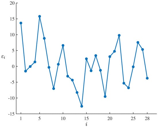
Figure 6. Residuals of the fitted uncertain FIFA football player valuation model (27) corresponding to the dataset $(y_i,x_{i1},x_{i2},x_{i3},x_{i4},x_{i5})$, $i=1,2,\cdots ,28$.

7. Conclusions

For the purpose of enriching the statistical inference study in uncertain regression analysis, a symmetric statistical invariant for the uncertain regression model based on observed data and uncertain disturbance terms was constructed in this paper. Based on the constructed statistical invariant, the least absolute deviation criterion was also applied to propose the least absolute deviation estimation for the uncertain regression model. Following that, the least absolute deviation estimation of the uncertain regression model was applied to the uncertain linear regression model, uncertain exponential growth model, and uncertain logistic decay model, respectively, and the advantages of the proposed method were also illustrated with two numerical examples by comparing with existing methods. Finally, the proposed method was also applied to two typical scenarios in sports statistics, and the corresponding uncertain statistical models were studied based on real data to illustrate the application effect.

In addition, future research directions could focus on the numerical solution algorithms for the corresponding least absolute deviation estimations, error analysis, and application research in typical cognitive uncertainty scenarios such as social statistics and psychostatistics.

References

- Galton, F. Family likeness in stature. Proc. R. Soc. Lond. 1886, 40, 42–73. [Google Scholar] [CrossRef]
- Draper, N.R.; Smith, H. Applied Regression Analysis, 2nd ed.; John Wiley and Sons: New York, NY, USA, 1981. [Google Scholar]
- Berkson, J. Application of the logistic function to bio-assay. J. Am. Stat. Assoc. 1944, 39, 357–365. [Google Scholar] [PubMed]
- Hoerl, A.; Kennard, R. Ridge regression: Biased estimation for nonorthogonal problems. Technometrics 1970, 12, 55–67. [Google Scholar] [CrossRef]
- Tibshirani, R. Regression shrinkage and selection via the lasso. J. R. Stat. Soc. Ser. Stat. Methodol. 1996, 58, 267–288. [Google Scholar] [CrossRef]
- Zou, H.; Hastie, T. Regularization and variable selection via the elastic net. J. R. Stat. Soc. Ser. B Stat. Methodol. 2005, 67, 301–320. [Google Scholar] [CrossRef]
- Freund, R.; Wilson, W.; Sa, P. Regression Analysis; Elsevier: Amsterdam, The Netherlands, 2006. [Google Scholar]
- Sen, A.; Srivastava, M. Regression Analysis: Theory, Methods and Applications; Springer Science & Business Media: Berlin/Heidelberg, Germany, 2012. [Google Scholar]
- Chatterjee, S.; Simonoff, J. Handbook of Regression Analysis; John Wiley & Sons: Hoboken, NJ, USA, 2013. [Google Scholar]
- Jiang, B.; Ye, T. Uncertain panel regression analysis with application to the impact of urbanization on electricity intensity. J. Ambient. Intell. Humaniz. Comput. 2023, 14, 13017–13029. [Google Scholar] [CrossRef]
- Liu, Y. Moment estimation for uncertain regression model with application to factors analysis of grain yield. Commun. Stat. Simul. Comput. 2024, 53, 4936–4946. [Google Scholar] [CrossRef]
- Liu, B. Uncertainty Theory, 2nd ed.; Springer: Berlin/Heidelberg, Germany, 2007. [Google Scholar]
- Liu, B. Some research problems in uncertainty theory. J. Uncertain Syst. 2009, 3, 3–10. [Google Scholar]
- Yao, K.; Liu, B. Uncertain regression analysis: An approach for imprecise observations. Soft Comput. 2018, 22, 5579–5582. [Google Scholar] [CrossRef]
- Ye, T.; Liu, Y.H. Multivariate uncertain regression model with imprecise observations. J. Ambient. Intell. Humaniz. Comput. 2020, 11, 4941–4950. [Google Scholar] [CrossRef]
- Chen, D. Uncertain regression model with autoregressive time series errors. Soft Comput. 2021, 25, 14549–14559. [Google Scholar] [CrossRef]
- Chen, D. Uncertain regression model with moving average time series errors. Commun. Stat. Theory Methods 2023, 52, 7632–7646. [Google Scholar] [CrossRef]
- Ding, J.; Zhang, Z. Statistical inference on uncertain nonparametric regression model. Fuzzy Optim. Decis. Mak. 2021, 20, 451–469. [Google Scholar] [CrossRef]
- Liu, Z.; Yang, Y. Least absolute deviations estimation for uncertain regression with imprecise observations. Fuzzy Optim. Decis. Mak. 2020, 19, 33–52. [Google Scholar] [CrossRef]
- Lio, W.; Liu, B. Uncertain maximum likelihood estimation with application to uncertain regression analysis. Soft Comput. 2020, 24, 9351–9360. [Google Scholar] [CrossRef]
- Liu, Y.; Qin, Z. Modified maximum likelihood approach in uncertain regression analysis and application to factors analysis of urban air quality. Math. Comput. Simul. 2025, 234, 219–234. [Google Scholar] [CrossRef]
- Chen, D. Tukey’s biweight estimation for uncertain regression model with imprecise observations. Soft Comput. 2020, 24, 16803–16809. [Google Scholar] [CrossRef]
- Lio, W.; Liu, B. Residual and confidence interval for uncertain regression model with imprecise observations. J. Intell. Fuzzy Syst. 2018, 35, 2573–2583. [Google Scholar] [CrossRef]
- Liu, Y.; Liu, B. A modified uncertain maximum likelihood estimation with applications in uncertain statistics. Commun. Stat. Theory Methods 2024, 53, 6649–6670. [Google Scholar]
- Liu, Y.; Liu, B. Estimation of uncertainty distribution function by the principle of least squares. Commun. Stat. Theory Methods 2024, 53, 7624–7641. [Google Scholar] [CrossRef]
- Ning, S.; Liu, Y. Estimation of unknown parameters in uncertainty distribution via the least absolute deviation principle and its application in uncertain statistics. Commun. Stat. Simul. Comput. 2025. accepted. [Google Scholar]
- Ye, T.; Liu, B. Uncertain hypothesis test with application to uncertain regression analysis. Fuzzy Optim. Decis. Mak. 2022, 21, 157–174. [Google Scholar] [CrossRef]
- Wang, H.; Liu, Y.; Shi, H. Estimating unknown parameters and disturbance term in uncertain regression models by the principle of least squares. Symmetry 2024, 16, 1182. [Google Scholar] [CrossRef]
- Li, C. The application of Excel multivariate linear regression in sports statistics. China Manag. Inform. 2011, 14, 65–66. [Google Scholar]
- FIFA23 Official Dataset. 2025. Available online: https://www.kaggle.com/datasets/bryanb/fifa-player-stats-database (accessed on 11 September 2025).
Disclaimer/Publisher’s Note: The statements, opinions and data contained in all publications are solely those of the individual author(s) and contributor(s) and not of MDPI and/or the editor(s). MDPI and/or the editor(s) disclaim responsibility for any injury to people or property resulting from any ideas, methods, instructions or products referred to in the content. |
© 2026 by the author. Licensee MDPI, Basel, Switzerland. This article is an open access article distributed under the terms and conditions of the Creative Commons Attribution (CC BY) license.