CPU-Only Spatiotemporal Anomaly Detection in Microservice Systems via Dynamic Graph Neural Networks and LSTM

Abstract

Microservice architecture has become a foundational component of modern distributed systems due to its modularity, scalability, and deployment flexibility. However, the increasing complexity and dynamic nature of service interactions have introduced substantial challenges in accurately detecting runtime anomalies. Existing methods often rely on multiple monitoring metrics, which introduce redundancy and noise while increasing the complexity of data collection and model design. This paper proposes a novel spatiotemporal anomaly detection framework that integrates Dynamic Graph Neural Networks (D-GNN) combined with Long Short-Term Memory (LSTM) networks to model both the structural dependencies and temporal evolution of microservice behaviors. Unlike traditional approaches, our method uses only CPU utilization as the sole monitoring metric, leveraging its high observability and strong correlation with service performance. From a symmetry perspective, normal microservice behaviors exhibit approximately symmetric spatiotemporal patterns: structurally similar services tend to share similar CPU trajectories, and recurring workload cycles induce quasi-periodic temporal symmetries in utilization signals. Runtime anomalies can therefore be interpreted as symmetry-breaking events that create localized structural and temporal asymmetries in the service graph. The proposed framework is explicitly designed to exploit such symmetry properties: the D-GNN component respects permutation symmetry on the microservice graph while embedding the evolving structural context of each service, and the LSTM module captures shift-invariant temporal trends in CPU usage to highlight asymmetric deviations over time. Experiments conducted on real-world microservice datasets demonstrate that the proposed method delivers excellent performance, achieving 98 percent accuracy and 98 percent F1-score. Compared to baseline methods such as DeepTraLog, which achieves 0.93 precision, 0.978 recall, and 0.954 F1-score, our approach performs competitively, achieving 0.980 precision, 0.980 recall, and 0.980 F1-score. Our results indicate that a single-metric, symmetry-aware spatiotemporal modeling approach can achieve competitive performance without the complexity of multi-metric inputs, providing a lightweight and robust solution for real-time anomaly detection in large-scale microservice environments.

1. Introduction

Modern large-scale software systems are increasingly adopting microservice architecture due to its modularity, scalability, and flexibility in development and deployment [1,2,3]. By decomposing applications into independently deployable services that interact through lightweight APIs, microservices enhance fault isolation and enable fine-grained resource management [4]. However, this shift introduces significant challenges in system reliability and anomaly detection. The high concurrency, decentralized deployment, and dynamic service topologies inherent in microservice systems make them particularly vulnerable to runtime anomalies such as resource exhaustion, cascading failures, and performance degradation.

In practice, microservice platforms generate diverse streams of monitoring data, including CPU usage, memory consumption, thread-pool statistics, service call traces, and logs [1]. While many existing anomaly detection methods rely on multi-metric fusion to characterize service behavior, this design often introduces feature redundancy, inconsistent update frequencies, and increased modeling complexity. Moreover, different metrics vary in sensitivity to anomalies and may interfere with each other when fused indiscriminately. These limitations raise a fundamental question: Are more features always better, or can fewer do more?

In this work, we explore a focused and lightweight alternative: modeling microservice anomalies using only CPU utilization as the input signal. This choice is driven by three observations: first, CPU usage is a low-level, high-frequency, and architecture-agnostic metric that directly reflects service workload and system stress; second, CPU fluctuations are sensitive to a wide range of anomalous events, such as deadlocks, overloads, and service crashes, and often exhibit spatial propagation along service-invocation chains; and third, by eliminating feature-level noise and heterogeneity, single-metric modeling enables simpler, more interpretable, and more deployable anomaly detection frameworks.

Existing methods, including log-oriented, RPC-based, and multi-metric GNN approaches, have made progress in anomaly detection for microservice systems, but they face several key limitations: Log-oriented methods: These methods focus on logs and trace data to capture inter-service communication patterns (e.g., DeepTraLog). However, they are not effective in detecting anomalies caused by resource bottlenecks (e.g., CPU overload, memory leaks), which often do not have associated log errors or trace anomalies. RPC-based methods: These methods rely on remote procedure call (RPC) patterns (e.g., Informer) to detect anomalies. While effective for handling communication delays and traffic patterns, they are limited by incomplete logs or data inconsistencies and assume stable call chains, which can be impacted by large data volumes or log accuracy issues. Multi-metric GNN methods: These approaches combine multiple metrics (e.g., CPU, memory, response times) for anomaly detection. While they provide multi-dimensional information, they often suffer from feature redundancy, noise, and inconsistent update frequencies, complicating data collection and model training. The gap addressed by this study is: How can we efficiently detect anomalies in microservice environments that are resource-constrained and require real-time monitoring, using only a single, low-cost metric (such as CPU utilization), and through spatiotemporal modeling (using D-GNN combined with LSTM), without relying on multiple redundant features or complex data sources? Existing methods often depend on heterogeneous signals (logs, RPCs, and multiple performance metrics), whereas this study proposes a lightweight anomaly detection framework focused solely on CPU utilization, a high-frequency, low-cost metric that directly reflects service load. Our experimental results show that this single-metric approach achieves performance comparable to multi-metric methods, without the additional overhead.

To fully exploit the dynamic and structural patterns encoded in CPU usage, we propose a framework that combines Dynamic Graph Neural Networks (D-GNNs) with Long Short-Term Memory (LSTM) networks. In our approach, microservices are represented as nodes, their interactions as evolving graph edges, and CPU usage as time-varying node attributes. The D-GNN module captures the temporal evolution of inter-service topology, embedding the structural context of each service, while the LSTM module learns sequential usage trends to identify temporal deviations. This design moves beyond conventional feature fusion by shifting the focus from feature-level representation to structure-aware, signal-centric modeling.

Extensive experiments on real-world microservice datasets show that the proposed method achieves detection accuracy on par with or superior to multi-metric baselines, while markedly reducing system complexity and enhancing interpretability. The findings indicate that deep modeling of a single, high-quality metric, when coupled with spatiotemporal abstraction, can outperform less expressive approaches that rely on multiple noisy features. This study provides not only a practical detection framework but also a conceptual advance toward simpler, more scalable, and robust anomaly detection in complex distributed systems.

The main contributions of this paper are summarized as follows:

• We propose the first dynamic GNN-based anomaly detection framework using only CPU utilization for microservices. This framework integrates dynamic graph neural networks (D-GNNs) and Long Short-Term Memory (LSTM) networks, using a single metric (CPU utilization) to achieve efficient spatiotemporal modeling. Unlike multi-metric methods such as DeepTraLog, which rely on multiple data sources (logs, traces, and performance metrics), our approach demonstrates that anomaly detection can be effectively achieved using only a single metric, simplifying the model while maintaining accuracy.
• We design a novel dynamic graph construction scheme, including hierarchical service layers (service types, deployment containers, service instances) and time-slice nodes for CPU usage at each time step, capturing the evolution of workloads and faults over time. Compared to static graph methods like MADM, which use fixed graph structures, our method integrates time-slice nodes to model temporal dynamics, significantly improving anomaly detection accuracy and robustness.
• We design a multi-stage resampling and SMOTE-based data preprocessing pipeline to address class imbalance in the ChaosStarBench dataset. This pipeline includes progressive temporal resampling and Synthetic Minority Over-sampling Technique (SMOTE) to augment minority class samples, improving anomaly discriminability and enhancing model robustness. While SMOTE is commonly used in imbalanced data learning, our approach uniquely adapts resampling techniques to the temporal nature of microservice CPU usage data, providing a more effective solution for detecting rare anomalies than methods like DeepTraLog.

Beyond the above contributions, we also reinterpret microservice anomaly detection from a symmetry perspective. The concept of symmetry is a central theoretical element in our framework, explaining how normal microservice behavior exhibits consistent spatiotemporal patterns. Under normal operation, the service interaction graph exhibits approximate structural symmetries, where services in similar roles show comparable dependency patterns and CPU utilization trajectories, while quasi-periodic workloads induce temporal symmetries such as repeated motifs and time-shift invariance.When an anomaly occurs in the system, this normal symmetry is disrupted, resulting in ‘symmetry-breaking events’. These events manifest as deviations in the CPU usage trajectories, where affected services no longer follow similar patterns or exhibit abnormally high or low CPU usage, creating localized structural and temporal asymmetries. Runtime anomalies break these spatiotemporal symmetries, creating localized structural and temporal asymmetries in the service graph. Within this view, our D-GNN–LSTM framework operates on a spatiotemporal graph whose nodes represent services, edges their interactions, and node features CPU utilization signals, with the GNN component preserving permutation symmetry over node relabeling and the temporal encoder capturing shift-invariant trends while remaining sensitive to symmetry-breaking deviations that indicate faults.

2. Related Work

2.1. Global Research

In recent years, GNNs have been widely adopted for anomaly detection in microservice systems to address the complexity of distributed environments by modeling diverse aspects of service behavior [5,6].

One representative line of work leverages system logs for anomaly detection [7]. A graph is constructed where log events (log type, occurrence time) and invocation events (synchronous and asynchronous calls) are represented as nodes, while sequential and invocation relations are modeled as edges. Each log trace encodes extensive invocation details with potentially complex structures. The method builds a trace graph that incorporates both log and invocation patterns, and applies Gated GNNs (GGNNs) [8] with Support Vector Data Description (SVDD) [9] for training. Normal behavior is characterized by the smallest hypersphere in the latent space, as defined by Deep SVDD, with deviations regarded as anomalies. While effective, this approach relies on integrating heterogeneous signals, which increases complexity and demands a carefully structured framework.

Another study combines GNNs with positive–unlabeled (PU) learning [7]. Features such as response codes, temporal attributes (duration, waiting time, relative start time), and semantic information are extracted, with invocation chains forming graph edges. GNNs capture structural dependencies, while PU learning leverages limited labeled data for training.

In addition, the Informer approach explores anomaly detection based on Remote Procedure Call (RPC) patterns [10]. This method applies DBSCAN [11] to extract invocation-chain patterns and then models each chain with DCRNN [12] for anomaly identification. Graph features include RPC identifiers, invocation frequency, service metadata, traffic statistics, and business characteristics. However, this approach requires large data volumes and assumes complete log accuracy, which is often unrealistic in practice.

Overall, existing GNN-based methods for microservice anomaly detection typically rely on multi-metric feature extraction. Few studies explore the potential of deeply modeling a single, high-quality metric such as CPU usage. The lack of such focused exploration leads to challenges in runtime data requirements, accuracy, and robustness. Moreover, limited attention has been paid to dynamic spatiotemporal mechanisms that could further enhance detection performance.

To address these gaps, this paper proposes a framework centered on dynamic spatiotemporal attention and the multidimensional characterization of CPU usage. The study examines whether integrating spatiotemporal dynamics with a single informative metric can achieve higher accuracy and robustness than approaches that rely on multiple noisy features.

2.2. Feature-Based Studies

The CPU is a fundamental component responsible for executing computational tasks, including user-level programs, operating-system calls, and hardware-interrupt handling. The overall system load is directly reflected in CPU usage [13]. Compared with higher-level indicators such as network latency or inter-service invocation time, CPU usage is closer to the hardware layer and provides a more direct and accurate reflection of performance and computational demand.

In microservice architectures, deployment typically relies on containers or virtual machines, with computational resources primarily allocated through CPU cores. CPU usage therefore serves as a key measure of microservice resource consumption [14]. Given the dynamic nature of microservice systems, CPU usage can sensitively capture fluctuations in resource utilization, offering essential support for performance optimization and load balancing.

The reliability of cpu.usage as a single feature lies in its precision and focus. It directly measures the utilization state of hardware resources, reflecting underlying computational behavior without the noise introduced by high-level indicators. Focusing on CPU usage enables more effective identification of abnormal states while reducing the complexity associated with multi-metric integration. This highlights CPU usage as a robust and interpretable indicator for anomaly detection.

2.3. Model-Based Research

LSTM networks are widely used for time-series modeling. As an extension of RNNs, LSTMs mitigate gradient issues and improve memory retention. An LSTM unit consists of three gates: the input gate, which regulates how much new information enters; the forget gate, which determines which past information is discarded; and the output gate, which controls the influence of the hidden state on the final output. These mechanisms allow LSTMs to capture long-term dependencies while filtering irrelevant information [15]. Variants such as Bi-LSTM further enhance sequence-pattern extraction by modeling temporal dependencies in both directions. For microservice environments with strong temporal dynamics, LSTMs provide an effective means of modeling sequential features.

GNNs have also demonstrated strong capabilities in modeling graph-structured data, particularly in static settings. Recent research extends them to dynamic GNNs, which incorporate temporal information to capture evolving graph topologies [16]. Dynamic GNNs are generally categorized into discrete models, which process graph snapshots at successive intervals, and continuous models, which update node representations in real time based on event sequences, often combined with recurrent architectures [17].

Combining LSTMs with dynamic GNNs provides a promising direction for anomaly detection in microservices. LSTMs capture temporal dependencies, while dynamic GNNs model evolving structural relationships among services. Our proposed model integrates these two components, using CPU usage as the sole monitoring feature. This framework, denoted as LSTM–Dynamic GNN, unifies temporal sequence modeling with graph-based structural learning to enhance anomaly detection in microservice systems.

2.4. Survey of GNN Applications in Microservice Anomaly Detection

While there are several studies using GNNs for logs (e.g., DeepTraLog for trace event graphs) and RPC (e.g., Informer for RPC pattern anomaly detection), there has been limited work on directly applying GNN or Dynamic GNN (D-GNN) to microservice anomaly detection, especially with a focus on CPU utilization as the sole metric. Notably, Ref. [18] provides an overview of how GNNs have been extended to dynamic settings but does not extensively cover how this applies to microservices. A more systematic discussion is necessary here to clarify the proximity of the proposed approach to these existing methods.

Closest Approaches to the Proposed Work: The closest existing work to the proposed method is MADM (Multi-Metric GNN for Anomaly Detection in Microservices). MADM uses multiple monitoring signals (CPU, memory, response time, etc.) and applies GNNs to detect anomalies in distributed systems. While MADM shares the use of GNNs, it does not explore the simplification of anomaly detection to a single metric (CPU utilization) and does not incorporate dynamic graph learning to model temporal dependencies. Another relevant approach is DeepTraLog, which integrates system logs with GNNs for anomaly detection. However, it depends heavily on logs and invocation events and does not focus on CPU utilization or dynamically adjusting graph structures based on evolving microservice behavior. Graph-based methods in microservice anomaly detection, such as GCN-based methods and Graph Convolutional Recurrent Networks (GCRN), have been used to model interactions in distributed systems. However, they typically rely on multi-metric features or focus on static graph representations without accounting for the temporal dynamics, which is a key feature of the proposed D-GNN + LSTM approach.

2.5. Comparative Discussion of Architectures and Features

Multi-Metric GNN Approaches: Approaches like MADM and others that rely on multiple features face several challenges, such as data redundancy, noise interference, and high model complexity. These methods tend to process a large number of metrics (e.g., CPU, memory, network, and logs) simultaneously, which can be computationally expensive and difficult to scale in real-world systems. Additionally, the challenge of maintaining consistency across different types of data, with varying update rates and sampling intervals, makes these models harder to deploy in dynamic environments.

Single-Metric GNN Approaches: In contrast, the proposed approach uses CPU utilization as the single metric. This makes the model simpler, more interpretable, and easier to deploy, as there is no need to manage and fuse multiple data sources. Furthermore, using CPU utilization—a high-frequency, architecture-agnostic, and direct reflection of service load—simplifies anomaly detection and allows for faster and more efficient monitoring. The D-GNN framework in our approach dynamically adapts to the structural and temporal evolution of the service graph, which makes it more robust to changes in microservice interactions compared to static GNN methods.

Dynamic Graph Neural Networks (D-GNNs): The use of D-GNNs in our approach is a significant innovation over static GNN methods. D-GNNs capture the temporal dynamics of microservice systems by evolving graph structures over time. This approach allows for more flexible and real-time anomaly detection compared to traditional GNN-based methods that treat the graph structure as static. This dynamism is critical for microservices, where service topologies and resource utilization fluctuate over time due to load balancing, scaling, and failures.

2.6. Research Gaps and Motivation

While there has been significant research on anomaly detection in microservices using multi-metric approaches (such as MADM and DeepTraLog), there remains a notable gap in systematically studying whether a single low-level metric (CPU utilization) can effectively outperform these multi-metric methods when incorporated into a dynamic graph-based framework. Most existing work relies on multi-metric fusion to capture a wide range of microservice behaviors. These methods often combine various features, such as CPU, memory, response times, and logs, assuming that the more data available, the better the performance. However, this approach introduces challenges such as feature redundancy, inconsistent update frequencies, and high model complexity, making it difficult to scale in real-time, large-scale microservice environments.

In contrast, the idea of using a single low-level metric, such as CPU utilization, as the sole input for anomaly detection has been largely underexplored. CPU utilization, being a low-level, high-frequency metric that reflects system load and performance, offers significant advantages in terms of observability, sensitivity to anomalies (such as deadlocks, overloads, and crashes), and simplicity in both data collection and model design. Despite its potential, there has been limited research on whether CPU-only anomaly detection can be as effective, or even outperform, multi-metric methods in the context of dynamic graph-based modeling. Specifically, dynamic graph neural networks (D-GNNs) offer a novel way to model temporal and structural dependencies in microservices, but no systematic study has been conducted to evaluate whether the combination of a single metric like CPU utilization with dynamic graphs can achieve competitive or superior performance compared to traditional multi-metric fusion methods.

This gap highlights a key research question: Can a single, low-level metric such as CPU utilization, when modeled with dynamic graphs, provide a more scalable, interpretable, and efficient solution for anomaly detection than methods that rely on multiple, potentially redundant features? Our work aims to fill this gap by demonstrating that a single-metric, dynamic graph-based approach can achieve anomaly detection performance comparable to or better than multi-metric approaches, while simplifying model complexity and improving interpretability.

3. Preliminaries

3.1. Microservice Architecture and Evolution

Microservices are a modern software architecture that decomposes applications into independent modules. These modules are developed, deployed, and maintained separately, with communication supported through lightweight APIs (Figure 1). The primary goal is to allow each core function within an application to operate independently, with individual modules focusing on specific tasks. This decoupling enables parallel development and improves efficiency [2]. During operation, failures in one module do not necessarily propagate to others, thereby enhancing fault isolation.

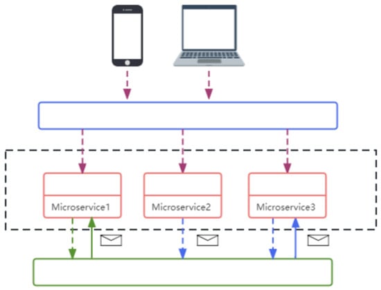
Figure 1. Overview of microservice architecture.

In contrast to monolithic architectures, where all functions are tightly integrated, microservices provide clear advantages. In a monolithic system, a fault in one function may affect the entire application. The evolution of architectures has moved from monolithic designs to Service-Oriented Architecture, which introduced partial modularization but retained shared dependencies, and ultimately to microservices, which emphasize stronger modular independence.

3.2. Challenges in Microservice Anomaly Detection

With the increasing scale and complexity of microservices, the volume and heterogeneity of monitoring data have made anomaly detection a critical challenge. Microservices deployed on distributed infrastructures such as containers and virtual machines form highly dynamic systems with complex interdependencies. Detecting anomalies requires analyzing diverse data sources, including service calls, thread-pool metrics, messages, and logs, to prevent fault propagation and ensure system reliability.

Traditional machine-learning methods can perform well in simpler environments but often fail to capture the spatial and temporal structures inherent in microservices. Consequently, there is a need for models that can jointly analyze spatial relationships and temporal dynamics to achieve robust anomaly detection in such environments.

3.3. GNNs in Microservice Anomaly Detection

Recent advancements in deep learning have introduced GNNs as effective tools for capturing spatial dependencies in graph-structured data. GNNs are well suited to scenarios where node counts vary, data formats are irregular, and adjacency relationships are complex. They have demonstrated strong performance in tasks such as node classification and link prediction [19], motivating their application to microservice anomaly detection.

The input to a GNN typically consists of a node-feature matrix, which captures node attributes, and an adjacency matrix, which encodes graph structure [20]. The output is a multi-dimensional representation of nodes that can be used for downstream tasks. In microservices, each service can be modeled as a node, with edges representing inter-service interactions. After training, GNNs generate latent feature vectors that characterize behavioral patterns of services. Normal operations form regular patterns, while anomalies manifest as deviations from these patterns, enabling effective detection.

Despite progress, several challenges remain. Nguyen et al. [18] emphasized that research on spatiotemporal GNNs and dynamic GNNs for microservice anomaly detection is still limited. Existing studies often neglect temporal dynamics, which are essential for accurately modeling the time-varying nature of microservice systems.

3.4. CPU Usage as a Feature

CPU usage is a fundamental metric for monitoring microservices, directly reflecting computational load at the hardware level. Under normal conditions, CPU usage remains relatively stable, while anomalies often cause significant deviations [13]. Compared with higher-level indicators, CPU usage offers a more direct and less noisy measure of system performance.

In microservice deployments, where computational resources are managed through CPU cores in containers or virtual machines, CPU usage provides a precise measure of resource consumption [14]. Its sensitivity to fluctuations makes it particularly useful for detecting abnormal states and supporting resource optimization.

Focusing solely on CPU usage minimizes redundancy and avoids the noise introduced by multiple correlated metrics. Unlike traditional approaches that rely on diverse monitoring signals, this study adopts CPU usage as a single indicator and integrates it with dynamic neural models. The proposed framework leverages temporal modeling through LSTMs and structural learning through GNNs to improve anomaly detection in microservice systems.

4. Data Processing

4.1. Data Introduction

The experiments are based on ChaosStarBench, an open-source benchmark for fault injection in cloud microservices. ChaosStarBench extends DeathStarBench, originally developed by the Packets and Complex Systems and Networks Labs at the University of Sussex [21]. The dataset covers four hours of operation. One hour after the start, a fault is injected into a single microservice instance and kept active for 45 min. During this period, three kinds of information were collected:

• Deployment: mapping of service instances to physical containers (e.g., service a-1, a-2, a-3 on containers m1–m5);
• CPU usage: utilization of each instance, sampled every 5 s;
• Call relationships and latency: invocation chains and response times (converted to milliseconds) at each sampling step.

To improve the clarity of the experimental setup, the following table will summarize the key parameters of the ChaosStarBench dataset:

Parameter	Description
Number of Services	26 services, 48 instances
Number of Containers	5 containers, each hosting multiple service instances
Fault Injection Types	Service crash, resource exhaustion, deadlock, service hang
Anomaly Types	CPU saturation, latency spikes, service crashes, resource exhaustion
Fault Injection Duration	Fault injected 1 h after system start, lasting for 45 min

Fault Injection Details: Fault injection occurs in the first hour after the start of data collection, targeting a single microservice instance. The fault types include service crash, resource exhaustion, deadlock, or service hang, among others. These faults cause significant fluctuations in performance metrics such as CPU utilization. The duration of the anomaly after fault injection is 45 min, during which the normal operation of the system is disrupted, and CPU utilization may experience a sharp increase or decrease. The 4 h dataset, which includes 45 min of error, proved sufficient for validating our method’s effectiveness. It captured typical service behavior and anomaly patterns without introducing excessive noise from larger datasets, making it representative for this study and demonstrating promise for real-world applications.

4.1.1. System Overview

The system consists of four layers: client, load balancer/front end, microservices, and storage. Our analysis focuses on the microservice layer. Figure 2 shows the deployment.

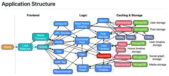
Figure 2. Node deployment overview.

4.1.2. Data Preparation

Monitoring gaps occasionally led to missing records, so resampling was necessary to obtain complete time series [22]. Three metrics were retained for further use:

• CPU usage (with timestamps),
• call duration (milliseconds),
• deployment status of each node.

Because anomalous samples were far fewer than normal ones, the data exhibited strong imbalance. To mitigate this, we used the Synthetic Minority Over-sampling Technique  [23] to generate additional minority-class samples before training.

4.2. Processing for Main Experiments

CPU usage. This was used as the main feature. Under normal conditions, values fluctuate within a narrow range. During faults they may rise sharply (extra resource demand) or collapse (service crash or hang), often coinciding with slow responses or restarts.

Resampling. The original sampling rate was 5 s, which might lead to missing or incomplete data in certain time periods. To ensure data integrity and improve temporal resolution, we resampled the data using a scheme of 5 s → 1 s → 500 ms, enhancing the model’s ability to capture temporal dynamic changes. The choice of a 1 s sampling interval strikes a balance between capturing rapid fluctuations in CPU usage and avoiding excessive data redundancy. A longer interval, such as 5 s, may miss important short-term changes, while a shorter interval (e.g., 500 ms) could introduce noise and increase computational complexity. Therefore, the 1 s interval was selected to provide sufficient temporal precision for anomaly detection without introducing unnecessary computational burdens. For missing values, we applied interpolation to fill them, ensuring continuity in the data. When the missing data rate exceeded 30 percent, the corresponding time period data were discarded to prevent significant impacts on the model training. After inspection, the missing value ratio was found to be generally within 5 percent. Figure 3 compares the results before and after resampling.

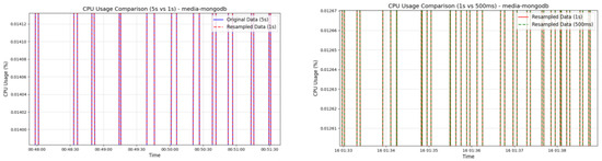
Figure 3. Zoomed-in comparison before and after resampling.

SMOTE. To address the class imbalance problem in the dataset, we adopted the Synthetic Minority Over-sampling Technique (SMOTE). SMOTE generates new samples by interpolating between minority class samples and their K nearest neighbors. These new samples are linear combinations of the original samples and their neighbors, which effectively increases the number of minority class samples in the training data and reduces the model’s bias toward the majority class.

Application of SMOTE in Time-Series Data:

Since SMOTE can lead to issues such as blurring of the time structure and information leakage between training and test sets, we applied the following measures:

SMOTE was applied only to the training set, after the initial data split. This ensured that synthetic samples were generated exclusively within the training data, preventing any leakage of information between the training and testing sets.

SMOTE was applied to minority class instances in the training set to balance the distribution of normal and anomalous states. Synthetic samples were generated before model training began, which improved the model’s ability to detect anomalies.

Temporal Integrity: SMOTE was applied carefully to maintain temporal dependencies. We avoided applying SMOTE to overlapping windows or windows where temporal continuity was essential, thus preserving the sequence of events in the time-series data.

Information Leakage: No synthetic data were introduced into the test set, maintaining its role as an unseen dataset for model evaluation. A stratified split was used to ensure consistent distributions of anomalies and normal states across training, validation, and test sets.

These steps ensured that the application of SMOTE did not introduce artifacts into the time-series data or compromise the evaluation process.

4.3. Processing for Comparison Experiments

Call duration. This feature records the time from request to completion. It is stable under normal conditions and increases once anomalies occur.

Aggregation. Raw data in milliseconds produced excessive volume. To make it usable, values were aggregated into fixed windows. Tests with 250 ms, 500 ms, and 1 s intervals showed that 250 ms created unnecessary overhead. A 1 s window was therefore adopted, which also aligned with the resampled CPU data.

5. Graph Construction

5.1. Principles of Graph Construction

The aim of this study is to construct a model that reflects both spatial and temporal patterns of microservice behavior. To achieve this, graphs are generated in a dynamic fashion: each time window produces a snapshot that records the system state. This approach enables temporal changes to be modeled alongside structural information, making it possible to trace how microservices evolve over time.

5.2. Graph Building Process

Graph quality has a direct influence on GNN performance, and the design here follows how microservices operate in practice. After several rounds of trial and error, we adopted a hierarchical structure with three main layers and additional temporal extensions.

As shown in Figure 4, service types form the top layer, deployment containers form the second, and individual service instances form the third. Containers are linked to the instances they host, and instances are linked back to their service type. From the fourth layer onward, time-slice nodes are added, recording CPU usage for each instance at every step in the window. This design keeps both the service hierarchy and the temporal dynamics in a single structure.

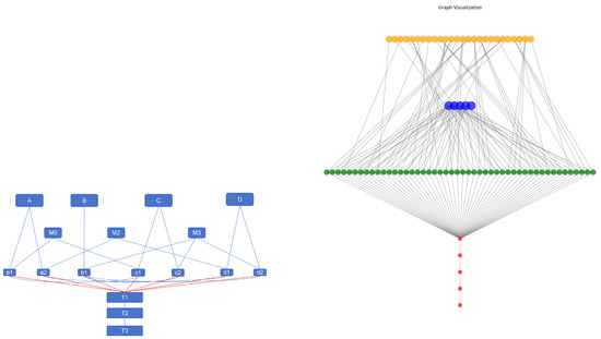
Figure 4. (Left): simplified sketch of the composition. (Right): Network visualization of the graph-construction scheme.

In this study, snapshots were generated every 5 s. This interval provided a balance: short enough to capture transient changes but long enough to avoid redundant information. Compared with static graphs, the dynamic setting was more effective in capturing how workloads and faults propagate across the system [24].

5.3. Dynamic Graph Construction

CPU usage data were first segmented into windows of length $T_w$. Each window was then expanded into a layered graph: service types, deployment containers, service instances, and time-slice nodes (one for each instance and each step within the window).

Edges connect types to their instances, containers to the instances they host, and each instance to its time-slice nodes. Consecutive time-slice nodes of the same instance are linked to preserve continuity. The resulting graphs are processed sequentially. Five consecutive snapshots are passed through the GCN encoder, and their outputs are then fed into an LSTM to capture longer temporal patterns. In practice, each snapshot is treated as an independent graph in the batch, while the LSTM handles the ordering.

To convert CPU utilization data into a dynamic graph structure, each microservice is represented as a node, with edges representing interactions between services. CPU utilization is used as the node attribute, and each time window corresponds to a graph snapshot. These snapshots capture the topological changes and interactions among services over time. Once the dynamic graphs are constructed, they are processed by the D-GNN component to capture spatial dependencies, and the outputs are passed to an LSTM for temporal modeling, thus capturing spatiotemporal dependencies in the data.

5.4. Computational Complexity and Scalability

The addition of time slices introduces a significant number of nodes to the graph, which can lead to higher computational costs, especially in large-scale microservices environments where there may be hundreds or thousands of instances. The graph construction process scales linearly with the number of microservices, instances, and time slices.

Computational Complexity Analysis: For each time window, a graph is generated with nodes representing the service instances and time-slice nodes for each instance at each time step. The number of nodes in each graph is proportional to:

$$\mathrm{Number}\mathrm{of}\mathrm{Nodes}\mathrm{per}\mathrm{Time}\mathrm{Window}=N\times M+N\times M\times W$$

(1)

where

• N is the number of microservices,
• M is the number of instances per microservice,
• W is the number of time steps per window.

The total number of edges in each graph depends on the relationships between service instances and time slices. The computational complexity of constructing the graph for one time window is approximately:

$$O\left(\right(N\times M)\times W)$$

(2)

For T snapshots (across multiple time windows), the total complexity would be:

$$O(T\times (N\times M)\times W)$$

(3)

This highlights that the time complexity grows linearly with the number of instances M, the number of time slices W, and the number of snapshots T.

Scalability Considerations: For large-scale systems, dynamically constructing time-sliced graphs becomes more computationally expensive. Here are some potential strategies for optimizing scalability:

• Window Size Reduction: Adjusting the window size W can control the number of time-slice nodes. Smaller window sizes will reduce the number of nodes per graph, but the trade-off is a potential loss of important temporal dynamics for anomaly detection.
• Graph Sparsity: In practice, service interactions are often sparse, so using sparse adjacency matrices can help reduce both memory usage and computational load.
• Parallelization and Distributed Computing: To handle large-scale systems, parallel computation methods can be employed to build and process graphs for different service instances or time windows concurrently, reducing computation time.

Model Efficiency:

Although constructing dynamic graphs can be computationally intensive, subsequent graph convolution and LSTM processing steps can be parallelized to efficiently handle large-scale data. Techniques like batched processing and optimized sparse matrix operations can improve memory usage and computational efficiency.

5.5. Design Considerations

Faults in microservices usually appear first at the instance level and then affect other components. For this reason, instances were kept as explicit nodes rather than aggregated, which increased sensitivity to local anomalies. Adding time-slice nodes allowed the model to track second-level fluctuations in CPU usage.

Experiments confirmed the importance of these dynamic steps. Static graphs that ignored time performed markedly worse. The dynamic formulation, by contrast, highlighted large deviations in CPU usage within a window and improved anomaly-detection accuracy.

5.6. Feature Extraction

CPU usage was chosen as the key feature. It measures the share of CPU capacity consumed by each instance over time. Under normal conditions, usage remains relatively stable, indicating spare computational headroom. During faults, usage may spike when processes demand excessive resources or fall sharply if services crash or hang. Such shifts often coincide with delays or restarts, making CPU usage a direct and reliable indicator.

Although other features were explored in comparison experiments, CPU usage alone proved sufficient when combined with the proposed dynamic graph framework.

6. Methodology

We propose a hybrid framework for anomaly detection in microservices that integrates dynamic graph neural networks with LSTM networks. The model is designed to capture both the evolving inter-service structure and the temporal variation in CPU usage. The overall workflow consists of graph construction, preprocessing and resampling, spatiotemporal representation learning, and anomaly classification.

6.1. Problem Formulation

Let ${\mathcal{G}}_t=({\mathcal{V}}_t,{\mathcal{E}}_t,{\mathbf{X}}_t)$ denote the microservice graph snapshot at time t, where ${\mathcal{V}}_t$ is the set of instances, ${\mathcal{E}}_t$ the set of invocation links, and ${\mathbf{X}}_t$ the node-feature matrix. Each node has a single feature, $f_{\mathrm{cpu}}$, representing CPU usage at time t.

Given a sequence of graphs $\{{\mathcal{G}}_1,\dots ,{\mathcal{G}}_T\}$, the objective is to learn node-level representations ${\mathbf{H}}_t$ that encode both spatial dependencies within ${\mathcal{G}}_t$ and temporal dependencies across snapshots. Each node is then classified as normal or anomalous.

6.2. Data Processing

Resampling. The original CPU usage was recorded at 5 s intervals. To better capture short-term variations, the series was resampled to 1 s, which provided finer temporal resolution without excessive data expansion.

Balancing. Because anomalies are rare, the dataset was highly imbalanced. To address this, the Synthetic Minority Over-sampling Technique [23] was applied during preprocessing.

6.3. Graph Construction

For each time window, a dynamic graph is created with three main components: service types, deployment containers, and service instances. Instances are linked both to their containers and to the corresponding service type. To capture the underlying structural symmetry, we embed these components to reflect how normal microservice behavior follows consistent spatiotemporal patterns. To capture temporal evolution, additional nodes are added for each instance at every time step within the window, annotated with CPU usage. We recognize that adding “time-slice” nodes will increase the graph size, but this design allows the model to capture finer-grained temporal changes in CPU utilization, which enhances anomaly detection accuracy. Graphs are generated sequentially, forming the dynamic input to the model.

All graphs are stored in serialized format containing node features, adjacency matrices, and labels, which facilitates parameter tuning and repeated experiments. Labels are assigned by majority voting within each window: if abnormal states dominate, the window is marked anomalous.

6.4. Graph Convolution Layers

Each snapshot is processed by graph convolution. Self-loops are added to retain node information, and adjacency matrices are normalized to avoid bias from high-degree nodes. Message passing then aggregates neighborhood information, producing updated node features. A linear transformation and ReLU activation follow, enabling the network to learn nonlinear structural patterns.

Pooling. To generate a compact graph-level representation, we adopt a mixed pooling strategy that combines mean and max pooling. Mean pooling preserves global context, while max pooling emphasizes strong local signals. Empirical testing showed this combination yielded the most stable performance.

6.5. Spatiotemporal Model

To capture sequential dynamics, the pooled graph embeddings from consecutive snapshots are passed to an LSTM. In our experiments, the sequence length was set to 5 graphs (equivalent to 25 s), which balanced detection accuracy with computational cost. The D-GNN component captures the structural symmetry in the service interaction graph, while the LSTM module identifies temporal deviations from this symmetry. This model effectively detects anomalies by recognizing “symmetry-breaking events,” where deviations from the normal spatiotemporal patterns occur.

The full model consists of three GCN layers, one LSTM layer, a fully connected classifier, dropout regularization, and a sigmoid output. Graphs are first encoded by GCNs, pooled, and reshaped. The resulting sequence is then processed by the LSTM to capture temporal patterns. The final hidden states are passed through the classifier for anomaly prediction.

6.6. Training and Evaluation

The dataset was split into training, validation, and test sets in a 50:25:25 ratio with stratified sampling. Binary cross-entropy was used as the loss function. Optimization was performed with Adam, which adaptively adjusts learning rates and converged reliably in our experiments.

Splitting by Time:

Since the dataset involves time-series data, we performed the data split by time rather than randomly splitting the instances. This approach ensures that the model is trained on past data and tested on future data, which is a more realistic scenario in real-world anomaly detection, where future anomalies are unknown and cannot be predicted in advance. The time-series split was performed as follows:

• The training set consists of the first 50% of the time window data.
• The validation set consists of the next 25%.
• The test set consists of the last 25% of the time window.

This temporal split ensures that the model is evaluated on unseen future data, helping prevent data leakage from the training set into the test set.

Ensuring No Overlap in Fault Injection Periods:

To ensure that fault injection periods do not overlap between the train/test sets, we carefully isolated the fault injection events in time. The fault injection occurs one hour after normal data collection begins, and we made sure that the anomalous periods from the fault injections were contained within a single train/test split. This separation ensures that no anomalies from the test set were seen by the model during training. By organizing the data this way, the test set represents unseen anomalies that the model has not been exposed to during training, which enhances the validity of the evaluation and mitigates the risk of overestimating the model’s performance.

K-Fold Cross-Validation:

To further improve the robustness and reliability of the results, we performed k-fold cross-validation on the training set. This allows the model to be trained and evaluated on different subsets of the data, reducing the possibility of overfitting to any particular subset and providing a more reliable estimate of the model’s performance. During each fold, the training and validation sets were again split temporally to avoid any overlap of fault injection periods between the folds. This also ensured that the model was exposed to a diverse set of data distributions, including various anomaly types. In summary, the data was split based on time, ensuring that the fault injection periods did not overlap between the training and test sets. Stratified sampling was used to maintain class balance, and k-fold cross-validation was applied to improve the robustness of the model evaluation. These steps ensure that the reported 98% accuracy values are not overly optimistic and reflect a more reliable performance estimate. Binary cross-entropy was used as the loss function. Optimization was performed with Adam, which adaptively adjusts learning rates and converged reliably in our experiments.

Threshold selection is important in binary anomaly detection. Following [25], we tested values in the range $[0.47, 0.52]$ to calibrate the classifier, which improved the balance between precision and recall. The detection threshold of 0.5 was chosen based on our experimental results, where it provided a good balance between precision and recall. In the context of this study, a fixed threshold effectively reduced false alarms and worked well for the dataset and environment tested. While we understand that in real-time systems an adaptive threshold may be more appropriate, for the scope of this paper, using a fixed threshold allowed us to simplify the model and demonstrate its core functionality effectively. The threshold was selected to balance performance and practical deployment.

6.7. Model Formulation

For each snapshot ${\mathcal{G}}_t$, the graph encoder ${\mathcal{F}}_G$ produces node embeddings:

$${\mathbf{H}}_t={\mathcal{F}}_G\left({\mathcal{G}}_t\right)=DGNN({\mathcal{V}}_t,{\mathcal{E}}_t,{\mathbf{X}}_t).$$

(4)

The temporal encoder ${\mathcal{F}}_T$ is an LSTM that consumes a sequence of embeddings:

$${\mathbf{z}}_t={\mathcal{F}}_T\left([{\mathbf{H}}_{t-k},\dots ,{\mathbf{H}}_t]\right).$$

(5)

The final classifier predicts the anomaly label with binary cross-entropy loss:

$$\mathcal{L}=-\sum _{t=1}^T\sum _{i=1}^{N_t}\left(y_i^{t}log{\widehat{y}}_i^t+(1-y_i^t)log(1-{\widehat{y}}_i^t)\right).$$

(6)

7. Experiments

This section presents the experimental evaluation of the proposed anomaly-detection framework. We first conduct a comparative study on feature selection to analyze different system metrics. We then proceed to the final experiment using the D-GNN–LSTM architecture with only cpu.usage, followed by ablation studies comparing different model variants. Finally, we provide a summary of the findings.

In our experiments, we focused on comparing different variants of our proposed model (such as CPU-only vs. CPU+Call Duration and LSTM vs. no LSTM) to clearly demonstrate the advantages of our approach in terms of simplicity and efficiency. These experiments aim to verify our core hypothesis: that using only a single high-quality feature (CPU utilization) combined with D-GNN and LSTM can achieve competitive performance compared to more complex multi-feature methods. By focusing on internal comparisons, we were able to demonstrate that our model not only performs well but also reduces complexity and improves deployability. While we acknowledge the value of comparing against state-of-the-art frameworks, the current design aims to show the baseline effectiveness of our approach.

7.1. Experiments on Feature Selection

To assess the role of feature design in anomaly detection, two settings were considered. The first relies exclusively on fine-grained cpu.usage data, while the second reduces this detail and incorporates call duration as an additional feature. However, based on our analysis of real-world microservice data, we found that CPU utilization alone effectively reflects performance fluctuations and is highly sensitive to various anomaly types (such as resource overload, deadlocks, crashes, etc.). Our comparative experiments demonstrate that using only cpu.usage achieves comparable or even better performance than models using multiple features, while maintaining simplicity and interpretability and avoiding the redundancy and noise that may arise from additional features. Therefore, we believe that using CPU utilization as the sole feature is both a reasonable and effective choice for anomaly detection in microservices.

Setup A: Using onlycpu.usage. In this configuration, graphs are constructed directly from detailed cpu.usage. Figure 5 illustrates the construction procedure: the left panel provides a schematic overview, and the right panel presents the corresponding implementation. Nodes M1–M5 denote the deployed microservice instances, A1–C2 correspond to instances within a selected time window, and T1–T(1+n) represent temporal states across consecutive steps.

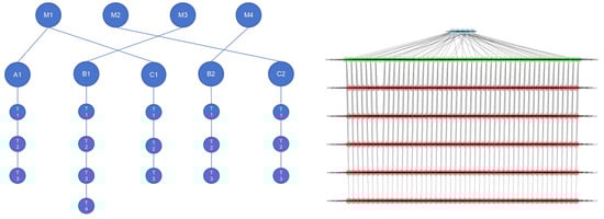
Figure 5. Graph construction and composition when only cpu.usage is used. (Left): simplified schematic. (Right): visualization of the composition code.

Setup B: Incorporating call duration. The second setup reduces part of the cpu.usage detail in each snapshot and adds call duration as an edge feature. Figure 6 shows the revised design. Compared with Setup A, this approach sacrifices some temporal and spatial resolution of cpu.usage to introduce communication-latency information. To ensure comparability and avoid confounding complexity, only GCNs are used in this comparison, with LSTMs excluded.

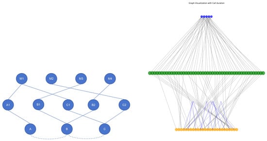
Figure 6. Graph construction and composition when both cpu.usage and call duration are used. (Left): simplified schematic. (Right): visualization of the composition code.

In this design, M1–M5 denote microservice deployments, A1–C2 represent instances within the time window, and A–C indicate service categories. Edge features E1 and E2 correspond to call duration between services.

Feature-selection results. Table 1 and Figure 7 compare the training results of the two setups. The model trained with only cpu.usage consistently outperforms the model that includes call duration. Figure 8, adapted from Giles [21], highlights the intuition: in the left panel, anomalies are clearly marked in cpu.usage (red interval), while in the right panel the corresponding call duration exhibits sharp spikes. To evaluate this effect, part of the fine-grained cpu.usage (from the third to nth-layer instances) was removed and replaced with call duration as edge attributes.

Table 1. Comparison of classification reports.

Class/Metric	CPU Only			CPU + Call Duration
	Precision	Recall	F1-Score	Precision	Recall	F1-Score
0	0.89	0.94	0.92	0.87	0.89	0.88
1	0.94	0.89	0.91	0.89	0.87	0.88
Accuracy	0.91			0.88
Macro avg	0.92	0.91	0.91	0.88	0.88	0.88
Weighted avg	0.92	0.91	0.91	0.88	0.88	0.88

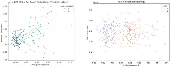
Figure 7. Comparison of PCA results: (Left) using only cpu.usage, with clear separation between classes; (Right) using cpu.usage with call duration, with weaker separation.

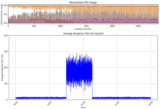
Figure 8. Illustration of anomalies in raw metrics. (Upper): cpu.usage with the anomalous interval marked in red. (Bottom): call duration with the corresponding anomalous spike.

Table 1 shows the cpu.usage-only model achieves higher precision, recall, and F1-score, especially for Class 0, where the precision and recall are 0.89 and 0.94, respectively. In contrast, the model with call duration shows lower precision and recall, particularly in the weighted averages. This suggests that the additional feature (call duration) introduces some noise that affects the model’s stability and performance.

PCA results, shown in Figure 7, further confirm the superiority of the cpu.usage-only model. On the left panel, the cpu.usage-only model demonstrates clear separation between normal and anomalous states, indicating better discriminability. On the other hand, the right panel, which includes call duration, shows weaker separation, reflecting the model’s reduced ability to distinguish between the two classes effectively. The cpu.usage-only model thus provides more informative features, leading to better performance in classification tasks.

Distinction Between Separated GNN-LSTM and Integrated D-GNN-LSTM:

To clarify the distinction between the separated GNN-LSTM and the integrated D-GNN-LSTM models, we describe their structural differences below.

7.2. Comparison with Literature Baselines

While the previous sections provided comparisons between different variants of our proposed approach, it is also crucial to compare our method with established baselines from the literature. In this section, we provide a comparison between our CPU-only D-GNN-LSTM model and existing methods, such as DeepTraLog (a log-oriented GNN method) and DBSCAN-based RPC methods like Informer (Table 2).

Table 2. Performance comparison with representative anomaly detection methods (higher is better).

Approach	Precision	Recall	F1-Score
TraceAnomaly	0.742	0.205	0.321
MultimodalTrace	0.591	0.776	0.671
DeepLog	0.608	0.948	0.741
LogAnomaly	0.415	0.977	0.582
GRU-based DeepSVDD	0.864	0.776	0.818
DeepTraLog	0.930	0.978	0.954
Our Method	0.980	0.980	0.980

7.2.1. Comparison with DeepTraLog and Log/Trace-Oriented GNN Approaches

DeepTraLog is a representative log and trace driven anomaly detection approach for microservice systems. It embeds span and log events, constructs a trace event graph (TEG) for each trace, and then performs graph-level anomaly detection using a GGNN-based Deep SVDD objective [26]. By leveraging rich observability signals, DeepTraLog reports strong detection performance (Precision = 0.930, Recall = 0.978, F1 = 0.954) [26].

In contrast, our method deliberately targets a metric-only setting and uses CPU utilization as the sole input signal. Despite the substantially reduced instrumentation and data requirements, our approach achieves competitive and even higher performance in the same evaluation protocol (Precision = 0.980, Recall = 0.980, F1 = 0.980). This comparison suggests that high-quality anomaly detection can be attainable under weaker observability assumptions, which is particularly valuable for production environments where logs and traces are incomplete, noisy, or costly to maintain.

Practical Advantages over DeepTraLog

• Lower observability and integration burden: DeepTraLog relies on both tracing and logging pipelines, whereas our method only requires CPU utilization, reducing deployment friction and improving applicability when only coarse-grained metrics are available.
• Time-varying interaction modeling: Our framework models microservice interactions with a dynamic graph that evolves over time, enabling the detector to capture temporal changes in service dependencies and workload conditions.
• Efficiency and scalability: Avoiding log parsing, event embedding, and per-trace graph construction substantially reduces computational overhead, making our approach easier to scale and operate under resource constraints.

7.2.2. Comparison with DBSCAN-Based RPC Methods (Informer)

Informer uses DBSCAN to detect anomalies based on RPC invocation chains, requiring complete and accurate log data, which can be challenging to obtain. In contrast, our CPU-only D-GNN-LSTM model simplifies data collection by relying solely on CPU utilization, making it more scalable and efficient.

Key Advantages of Our Method Over DBSCAN-based RPC Methods:

• Simplicity and Scalability: DBSCAN-based methods like Informer require extensive log data, while our method is simpler and more scalable, using only CPU utilization.
• Dynamic Adaptation: DBSCAN is a static clustering method, while our D-GNN and LSTM model dynamically adapts to evolving microservice interactions, capturing both temporal and structural dependencies.

By comparing our model with both DeepTraLog and DBSCAN-based methods like Informer, we demonstrate that our approach is not only simpler but also more scalable, efficient, and interpretable. The single-metric anomaly detection based solely on CPU utilization offers a lightweight solution for real-time anomaly detection in large-scale microservice environments.

7.3. Experiments on Our Method

Based on the above findings, the final experiment employs only cpu.usage as input to the D-GNN–LSTM framework. Raw data collected at 5 s intervals were resampled to 1 s intervals to enhance temporal resolution. Dynamic graphs were then constructed following the methodology described earlier, enabling the model to capture both spatial and sequential dependencies.

Experimental parameters. Hyperparameter Sensitivity Analysis We tested several hyperparameters to optimize the anomaly detection model. The following experiments were conducted to assess the impact of key hyperparameters and determine the best configuration for the model: In this study, we conducted a hyperparameter sensitivity analysis to assess the impact of key hyperparameters on the model’s performance. We tested three hyperparameters: sampling interval, window size, and LSTM sequence length. First, for the sampling interval, we experimented with 5 s, 1 s, and 500 ms, and found that a 1 s interval provided the best balance between capturing system behavior fluctuations and computational efficiency. The 500 ms interval introduced too much noise, impairing model stability, while the 5 s interval failed to capture fine-grained temporal changes. Next, for the window size, we tested 3 s, 5 s, and 10 s. The 5 s window offered sufficient context for accurate anomaly detection, while the 3 s window lacked enough context and the 10 s window caused data over-smoothing, reducing short-term anomaly detection capability. Finally, for the LSTM sequence length, we tested sequences of 3, 5, 8, and 10 snapshots. The 5-snapshot sequence provided the best trade-off between capturing temporal dependencies and avoiding overfitting, while shorter sequences (3) missed important temporal patterns, and longer sequences (8–10) led to overfitting and longer training times. Based on these experiments, we selected the optimal hyperparameter values to ensure the model captures significant system behavior fluctuations while maintaining both efficiency and stability.

The final configuration adopted a 1 s sampling interval, a 5 s window size, and an LSTM sequence length of 5. Hyperparameter analysis indicated that the window size was critical: performance degraded outside the range of 5–10 s. After balancing, the dataset covered approximately 6.5 h of runtime data. Optimal results were achieved with sequence lengths of 5–8, hidden dimensions of 96–128, batch sizes of 8–16, and 16–32 LSTM units. Training stabilized after 30–40 epochs, and the detection threshold was set to 0.5.

Results and analysis. Figure 9, Figure 10, Figure 11, Figure 12, Figure 13 and Figure 14 report the results of the final experiment. Training and validation losses decrease steadily with minimal overfitting (Figure 9), and accuracy improves consistently across epochs. The confusion matrix (Figure 13) confirms that most predictions are correct. The PCA projection further shows that embeddings of normal and anomalous states are clearly separated after training. The classification report (Table 3) and ROC curve (Figure 14) indicate strong and stable discriminative capability. Overall, the D-GNN–LSTM model using only cpu.usage achieves highly accurate anomaly detection, outperforming approaches that rely on larger sets of generalized features.

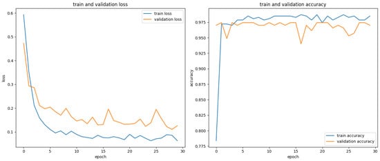
Figure 9. Training process of the final model. (Left): training and validation loss curves, showing gradual convergence with minimal overfitting. (Right) training and validation accuracy curves, indicating stable improvement over epochs.

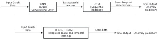
Figure 10. Distinction Between Two Model.

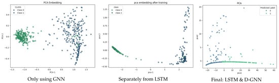
Figure 11. PCA embedding comparison across model variants.

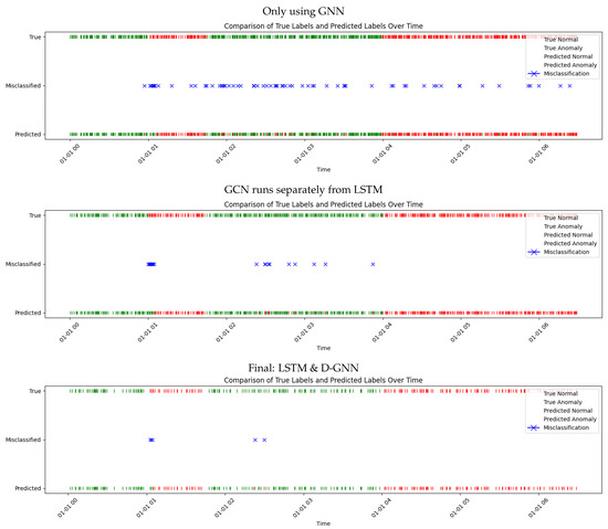
Figure 12. Label visualization over time for different model variants.

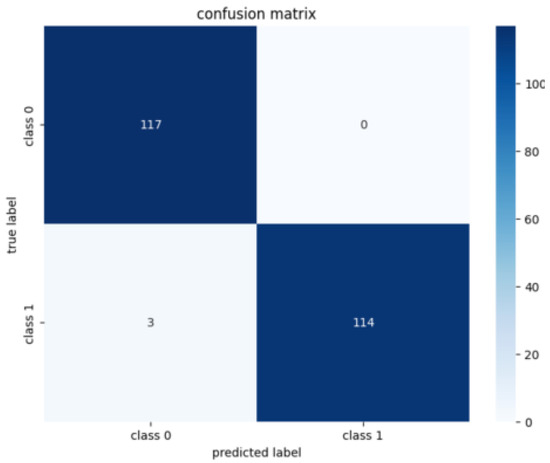
Figure 13. Confusion matrix of the final model. Most predictions align with ground truth, indicating strong classification performance.

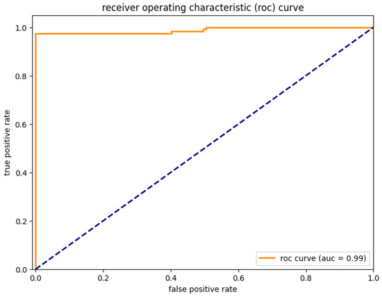
Figure 14. ROC curve and AUC of the final model, showing robust discriminative ability.

Table 3. Classification report of the final model, demonstrating balanced performance across normal and anomalous classes.

	Precision	Recall	F1-Score
Class 0	0.96	1.00	0.98
Class 1	1.00	0.96	0.98
Accuracy	0.98
Macro Avg	0.98	0.98	0.98
Weighted Avg	0.98	0.98	0.98

7.4. Further Analysis on Model Selection

To further investigate the role of temporal modeling, three configurations were compared: (i) a GCN-only model without LSTM, (ii) a separated GNN–LSTM model where spatial and temporal dependencies are processed independently, and (iii) the integrated D-GNN–LSTM model (Table 4).

Table 4. Classification report comparison across model variants.

Metric	Only Using GNN	GCN Separate from LSTM	Final: LSTM & D-GNN
Class 0 Precision	0.91	0.96	0.97
Class 0 Recall	0.90	0.96	0.98
Class 0 F1-score	0.91	0.96	0.98
Class 1 Precision	0.90	0.96	0.98
Class 1 Recall	0.91	0.96	0.97
Class 1 F1-score	0.91	0.96	0.98
Accuracy	0.91	0.96	0.98
Macro avg (P/R/F1)	0.91/0.91/0.91	0.96/0.96/0.96	0.98/0.98/0.98
Weighted avg (P/R/F1)	0.91/0.91/0.91	0.96/0.96/0.96	0.98/0.98/0.98

The GCN-only model captures spatial structure but fails to exploit sequential dependencies: predicted labels exhibit frequent misclassifications, and PCA separation is limited. By contrast, the separated GNN–LSTM model improves considerably, revealing clearer class boundaries, fewer misclassifications, and better alignment of predicted and true labels. Nevertheless, the integrated D-GNN–LSTM model remains superior, confirming that spatial and temporal dependencies are best captured jointly.

Summary of model comparison. The comparative experiments reveal a clear trajectory of improvement: the GCN-only model achieves the lowest accuracy, the separated GNN–LSTM model performs better, and the integrated D-GNN–LSTM model delivers the best results. PCA embeddings illustrate this progression, with increasingly distinct clustering of normal and anomalous states. These results confirm that microservice anomaly detection benefits most from the joint modeling of dynamic spatial and temporal dependencies.

7.5. Discussion and Reflection

On graph construction. Graph construction begins with microservice deployment and layering, producing a hierarchical structure. Edges are designed to highlight relationships that differ between normal and abnormal states. Capturing these differences over time proves more effective than analyzing static snapshots, hence the adoption of a 5 s dynamic window.

From a practical perspective, merging multiple instances into single nodes can simplify the model but at the cost of sensitivity. By focusing on cpu.usage, we balance simplicity with discriminative power, which is advantageous for deployment.

On feature selection. The experiments consistently show that fine-grained cpu.usage is more informative than additional metrics such as call duration. This reinforces the idea that a single, high-quality metric, when modeled carefully, may outperform multiple less-informative features. In our experiments, we observed that incorporating ‘Call Duration’ as an additional edge feature slightly reduced performance due to suboptimal integration of this feature. However, this does not imply that adding multiple features always introduces noise. We focused on cpu.usage as the sole feature because it directly and reliably reflects system performance, making it sufficient for detecting most anomalies. By simplifying the feature set to focus on CPU utilization, we improved both model accuracy and interpretability. The finding also aligns with neural-network practice, where selecting and refining core variables often yields better generalization.

On model choice. As illustrated in Table 2, the proposed D-GNN–LSTM model outperforms all baselines, reaching 98% accuracy with only cpu.usage. The integration of spatial and temporal representations is the key driver of this improvement.

7.6. Reflection on Findings

The results confirm that combining D-GNNs with LSTMs yields a precise and stable anomaly-detection framework. The approach demonstrates that careful modeling of a single feature, coupled with dynamic graph construction and sequential encoding, provides more reliable outcomes than more complex feature sets.

7.7. Limitations

Despite its strong performance, the model is sensitive to specific service instances and may require retraining when applied to unseen microservice types. Microservice architectures are inherently dynamic, with service instances exhibiting diverse load patterns, configurations, and resource requirements. These differences can make it challenging for the model to immediately adapt to new instances, especially when their CPU utilization patterns deviate significantly from those seen during training. For instance, services handling high-frequency requests might display different CPU utilization fluctuations, which could affect the model’s performance. Additionally, the CPU utilization of each microservice depends on a variety of factors, including its own resource demands, load patterns, and inter-service dependencies. Variations in deployment environments (e.g., containers, virtual machines, or physical hosts) can lead to differences in CPU utilization patterns, which may further impact the model’s ability to generalize across various service instances.

While some anomalies, such as deadlocks or service configuration errors, may not significantly affect CPU utilization, we chose CPU utilization as the primary metric due to its reliability as a low-level, high-frequency indicator that reflects system load and health. CPU load fluctuations are commonly associated with performance bottlenecks and resource consumption anomalies, making it an effective and intuitive metric for anomaly detection in microservices. By focusing on CPU utilization, we avoid the complexity and potential noise introduced by multiple features, ensuring both model simplicity and efficiency. This design makes the model highly practical for real-world applications where CPU-related anomalies are predominant.

The model’s sensitivity to specific service instances means that new services may require retraining. This is a typical challenge in anomaly detection systems, particularly in dynamic environments where service instances frequently change. However, for most common service types, our model provides reliable anomaly detection, making it effective across a wide range of microservice environments. The need for retraining is a reasonable trade-off, considering the model’s accuracy and simplicity. Expanding the training dataset with more diverse anomaly patterns could further enhance its robustness. Another limitation is that LSTM-based sequence modeling may reduce temporal granularity, suggesting that future work could explore localized detection strategies to complement the current approach.

On dynamic service topologies. Microservices often evolve in response to factors such as load balancing, scaling, and failures. Our D-GNN-LSTM model is designed to adapt to such dynamic changes in service topology by leveraging the D-GNN component to capture evolving structural dependencies. However, when drastic changes occur—such as the addition or removal of services—the model may experience temporary performance degradation until it can adjust to the new topology. To address this, we suggest exploring online learning or incremental updates, which could allow the model to continuously adapt without requiring full retraining.

On adaptability to other metrics. Although our model currently uses CPU utilization, it can easily be extended to other metrics, such as memory usage or response time, by modifying the feature extraction pipeline and adjusting the graph construction process. This flexibility makes the model adaptable to various monitoring metrics commonly used in microservice environments, allowing it to scale across different types of system data.

On vulnerability to latency or log-based anomalies. While the CPU-only approach is effective for detecting CPU-related anomalies, it may struggle with anomalies that manifest in latency or logs but do not significantly impact CPU usage. For example, latency-induced performance degradation or log anomalies might not be captured effectively by our current model. Future work could explore integrating multiple metrics, such as latency or log data, to improve robustness and provide a more comprehensive anomaly detection framework. Alternatively, a hybrid model could be developed to combine CPU utilization with other signals, ensuring the model remains both efficient and flexible for various types of anomalies.

8. Conclusions

This study introduces a microservice anomaly-detection framework that relies solely on cpu.usage as the input feature, integrating dynamic graph neural networks with long short-term memory networks. Extensive experiments demonstrate that this design achieves excellent detection performance, reaching 98% in both accuracy and F1-score. The findings confirm that CPU utilization, as a fundamental system metric, provides sufficient information to distinguish between normal and anomalous service states.

Comparative analyses further show that detailed modeling of cpu.usage often surpasses approaches that incorporate additional features such as call duration. This observation suggests that carefully refining a single informative feature can sometimes yield better anomaly-detection outcomes than combining multiple heterogeneous inputs. Moreover, the integrated D-GNN–LSTM architecture consistently outperforms alternative model variants, including GCN-only and separated GCN–LSTM baselines, highlighting the advantage of jointly capturing spatial dependencies and temporal dynamics in microservice systems.

The results also carry methodological implications. They demonstrate that effective anomaly detection does not necessarily require complex feature sets; instead, it can be achieved through precise construction of dynamic graphs and the integration of spatiotemporal representations. In practice, this reduces reliance on broad monitoring metrics while maintaining high detection reliability, offering a more efficient path for real-world deployment in complex microservice environments.

Looking ahead, future work will aim to enhance the generalization ability of the model by refining graph-construction strategies, incorporating additional temporal descriptors to capture richer sequential patterns, and investigating cross-system transferability to strengthen robustness under diverse anomaly types and deployment scenarios.

References

- Jamshidi, P.; Pahl, C.; Mendonça, N.C.; Lewis, J.; Tilkov, S. Microservices: The journey so far and challenges ahead. IEEE Softw. 2018, 35, 24–35. [Google Scholar] [CrossRef]
- Sampaio, A.R.; Kadiyala, H.; Hu, B.; Steinbacher, J.; Erwin, T.; Rosa, N.; Beschastnikh, I.; Rubin, J. Supporting microservice evolution. In Proceedings of the 2017 IEEE International Conference on Software Maintenance and Evolution (ICSME), Shanghai, China, 17–22 September 2017; pp. 539–543. [Google Scholar]
- Yang, H.; Zhou, Y. Ida-gan: A novel imbalanced data augmentation gan. In Proceedings of the 2020 25th International Conference on Pattern Recognition (ICPR), Milan, Italy, 10–15 January 2021; pp. 8299–8305. [Google Scholar]
- Dragoni, N.; Giallorenzo, S.; Lafuente, A.L.; Mazzara, M.; Montesi, F.; Mustafin, R.; Safina, L. Microservices: Yesterday, today, and tomorrow. In Present and Ulterior Software Engineering; Springer: Cham, Switzerland, 2017; pp. 195–216. [Google Scholar]
- Wang, M.; Yang, H.; Cheng, Q. Gcl: Graph calibration loss for trustworthy graph neural network. In Proceedings of the 30th ACM International Conference on Multimedia, Lisboa, Portugal, 10–14 October 2022; pp. 988–996. [Google Scholar]
- Wang, M.; Yang, H.; Huang, J.; Cheng, Q. Moderate message passing improves calibration: A universal way to mitigate confidence bias in graph neural networks. In Proceedings of the AAAI Conference on Artificial Intelligence, Vancouver, BC, Canada, 26–27 February 2024; Volume 38, pp. 21681–21689. [Google Scholar]
- Zhang, K.; Zhang, C.; Peng, X.; Sha, C. Putracead: Trace anomaly detection with partial labels based on gnn and pu learning. In Proceedings of the 2022 IEEE 33rd International Symposium on Software Reliability Engineering (ISSRE), Charlotte, NC, USA, 31 October–3 November 2022; pp. 239–250. [Google Scholar]
- Groh, F.; Ruppert, L.; Wieschollek, P.; Lensch, H.P. Ggnn: Graph-based gpu nearest neighbor search. IEEE Trans. Big Data 2022, 9, 267–279. [Google Scholar] [CrossRef]
- Yi, J.; Yoon, S. Patch svdd: Patch-level svdd for anomaly detection and segmentation. In Proceedings of the Asian Conference on Computer Vision, Kyoto, Japan, 30 November–4 December 2020. [Google Scholar]
- Chen, J.; Huang, H.; Chen, H. Informer: Irregular traffic detection for containerized microservices RPC in the real world. In Proceedings of the 4th ACM/IEEE Symposium on Edge Computing, Washington, DC, USA, 7–9 November 2019; pp. 389–394. [Google Scholar]
- Schubert, E.; Sander, J.; Ester, M.; Kriegel, H.P.; Xu, X. DBSCAN revisited, revisited: Why and how you should (still) use DBSCAN. ACM Trans. Database Syst. (TODS) 2017, 42, 1–21. [Google Scholar] [CrossRef]
- Zhou, J.; Yu, Q. Dcrnn: A deep cross approach based on rnn for partial parameter sharing in multi-task learning. arXiv 2023, arXiv:2310.11777. [Google Scholar] [CrossRef]
- Chen, S.; Shen, Y.; Zhu, Y. Modeling conceptual characteristics of virtual machines for CPU utilization prediction. In Proceedings of the International Conference on Conceptual Modeling, Xi’an, China, 22–25 October 2018; Springer: Berlin/Heidelberg, Germany, 2018; pp. 319–333. [Google Scholar]
- Erikson, W.J. The value of CPU utilization as a criterion for computer system usage. ACM SIGMETRICS Perform. Eval. Rev. 1974, 3, 180–187. [Google Scholar] [CrossRef]
- Greff, K.; Srivastava, R.K.; Koutník, J.; Steunebrink, B.R.; Schmidhuber, J. LSTM: A search space odyssey. IEEE Trans. Neural Netw. Learn. Syst. 2016, 28, 2222–2232. [Google Scholar] [CrossRef] [PubMed]
- Feng, Z.; Wang, R.; Wang, T.; Song, M.; Wu, S.; He, S. A comprehensive survey of dynamic graph neural networks: Models, frameworks, benchmarks, experiments and challenges. arXiv 2024, arXiv:2405.00476. [Google Scholar] [CrossRef]
- Zheng, Y.; Yi, L.; Wei, Z. A survey of dynamic graph neural networks. Front. Comput. Sci. 2025, 19, 196323. [Google Scholar] [CrossRef]
- Nguyen, H.X.; Zhu, S.; Liu, M. A survey on graph neural networks for microservice-based cloud applications. Sensors 2022, 22, 9492. [Google Scholar] [CrossRef] [PubMed]
- Zhou, J.; Cui, G.; Hu, S.; Zhang, Z.; Yang, C.; Liu, Z.; Wang, L.; Li, C.; Sun, M. Graph neural networks: A review of methods and applications. AI Open 2020, 1, 57–81. [Google Scholar] [CrossRef]
- Meng, C.; Song, S.; Tong, H.; Pan, M.; Yu, Y. Deepscaler: Holistic autoscaling for microservices based on spatiotemporal gnn with adaptive graph learning. In Proceedings of the 2023 38th IEEE/ACM International Conference on Automated Software Engineering (ASE), Luxembourg, 11–15 September 2023; pp. 53–65. [Google Scholar]
- Gan, Y.; Zhang, Y.; Cheng, D.; Shetty, A.; Rathi, P.; Katarki, N.; Bruno, A.; Hu, J.; Ritchken, B.; Jackson, B.; et al. An open-source benchmark suite for microservices and their hardware-software implications for cloud & edge systems. In Proceedings of the Twenty-Fourth International Conference on Architectural Support for Programming Languages and Operating Systems, Providence, RI, USA, 13–17 April 2019; pp. 3–18. [Google Scholar]
- Burnaev, E.; Erofeev, P.; Papanov, A. Influence of resampling on accuracy of imbalanced classification. In Proceedings of the Eighth International Conference on Machine Vision (ICMV 2015), Barcelona, Spain, 19–21 November 2015; SPIE: Bellingham, WA, USA, 2015; Volume 9875, pp. 423–427. [Google Scholar]
- Chawla, N.V.; Bowyer, K.W.; Hall, L.O.; Kegelmeyer, W.P. SMOTE: Synthetic minority over-sampling technique. J. Artif. Intell. Res. 2002, 16, 321–357. [Google Scholar] [CrossRef]
- Kazemi, S.M.; Goel, R.; Jain, K.; Kobyzev, I.; Sethi, A.; Forsyth, P.; Poupart, P. Representation learning for dynamic graphs: A survey. J. Mach. Learn. Res. 2020, 21, 1–73. [Google Scholar]
- Powers, D.M. Evaluation: From precision, recall and F-measure to ROC, informedness, markedness and correlation. arXiv 2020, arXiv:2010.16061. [Google Scholar] [CrossRef]
- Zhang, C.; Peng, X.; Sha, C.; Zhang, K.; Fu, Z.; Wu, X.; Lin, Q.; Zhang, D. Deeptralog: Trace-log combined microservice anomaly detection through graph-based deep learning. In Proceedings of the 44th International Conference on Software Engineering, Pittsburgh, PA, USA, 25–27 May 2022; pp. 623–634. [Google Scholar]
Disclaimer/Publisher’s Note: The statements, opinions and data contained in all publications are solely those of the individual author(s) and contributor(s) and not of MDPI and/or the editor(s). MDPI and/or the editor(s) disclaim responsibility for any injury to people or property resulting from any ideas, methods, instructions or products referred to in the content. |
© 2026 by the authors. Licensee MDPI, Basel, Switzerland. This article is an open access article distributed under the terms and conditions of the Creative Commons Attribution (CC BY) license.