A High-Performance Stochastic Framework for Landslide Uncertainty Analysis Using the Material Point Method and Random Field Theory

Abstract

This study proposes a novel high-performance computational framework to address the computational challenges in probabilistic large-deformation landslide analysis. By integrating a GPU-accelerated material point method (MPM) solver with a parallelized covariance matrix decomposition (CMD) algorithm for decomposing symmetric matrices, the framework achieves exceptional efficiency, demonstrating speedups of up to 532× (MPM solver) and 120× (random field generation) compared to traditional serial methods. Leveraging this efficiency, extensive Monte Carlo simulations (MCSs) were conducted to quantify the effects of spatial variability in soil properties on landslide behaviors. Quantitative results indicate that runout and influence distances follow normal distributions, while sliding mass volume exhibits log-normal characteristics. Crucially, deterministic analysis was found to systematically underestimate the hazard; the probabilistic mean sliding volume significantly exceeded the deterministic value, with 73–80% of stochastic realizations producing larger failures. Furthermore, sensitivity analyses reveal that increasing the coefficient of variation (COV) and the cross-correlation coefficient (from −0.5 to 0.5) leads to a monotonic increase in both the mean and standard deviation of large-deformation metrics. These findings confirm that positive parameter correlation amplifies failure risk, providing a rigorous physics-based basis for conservative landslide hazard assessment.

1. Introduction

Landslides are among the most widespread and destructive geological hazards worldwide. They not only pose a direct threat to human lives and infrastructure, but the resulting debris accumulation can also trigger secondary disasters. Historical events illustrate their devastating potential: in 1963, a landslide of over 270 million m³ from the Vaiont Dam reservoir in Italy generated a 220 m high wave, claiming more than 2000 lives downstream [1]; in 2003, the Qianjiangping landslide in China produced impulsive waves with amplitudes up to 40 m, collapsing 1100 structures and causing 14 fatalities [2]; in 2014, the Oso landslide (USA) engulfed 2.6 km², killing 43 people and destroying 49 homes [3]; and in 2020, a landslide in Kerala, India, traveled approximately 1200 m, affecting over 70,000 m² and resulting in 66 deaths [4]. These cases highlight that casualties and structural damage are often closely related to the large-deformation characteristics of slopes [5], including runout distance, collapse extent, and failure volume. Thus, accurately modeling large deformation behavior is critical for assessing hazard impact.

The spatial variability of mechanical parameters of soils arises primarily from long-term geological sedimentation, weathering cycles, hydraulic erosion, and anthropogenic disturbances, which collectively lead to heterogeneous material properties across different spatial locations. In order to capture and characterize the spatial variability of soils, autocorrelation functions (ACFs) are generally used to quantify soil parameter information gathered from in situ and laboratory tests [6,7,8]. Using ACFs, various deposited fabric patterns of spatially variable soils can be theoretically reproduced [9,10]. In stochastic analysis, several techniques are commonly employed, including the Karhunen–Loève (KL) expansion [11], local average subdivision (LAS) [12], and CMD [13]. The advantages and disadvantages of different methods are summarized in Table 1.

Table 1. Summary of the discrete technology of random fields used in geotechnics.

Discrete Technology of Random Fields	Advantages	Disadvantages
K-L	Efficient and accurate [11]	Accuracy depends on the value of the truncation term [14]
LAS	Efficient and accurate [15]	Has a systematic bias in the variance field [15] and is difficult to implement [16]
CMD	Simple to implement and accurate [16]	Relatively time-consuming for simulating large-scale random fields [16,17]

As shown in Table 1, compared to other random field generation methods, CMD is easier to use, which has led to its widespread application in non-deterministic analysis in geotechnical engineering. However, due to the substantial computational cost and time required, decomposing a significantly large multidimensional autocorrelation matrix using this method remains challenging. Therefore, it is necessary to highlight an improved approach to enhance the computational efficiency of CMD.

In recent years, probabilistic research has primarily aimed to characterize slope instability and the corresponding probability of failure using methods such as the limit equilibrium method (LEM) [18,19,20], finite element method (FEM) [21,22,23], and finite difference method (FDM) [24,25,26]. However, probabilistic analysis of post-failure slope behavior remains relatively limited, mainly due to (i) the rigid-body assumption inherent in the limit equilibrium method and (ii) computational instabilities induced by mesh distortion in mesh-based methods, both of which restrict the application of conventional approaches to large-deformation problems in slope engineering.

Recent developments in advanced numerical techniques such as Smoothed Particle Hydrodynamics (SPHs) [27,28,29], the MPM [30,31], and the Coupled Eulerian–Lagrangian (CEL) method [32,33] allow for robust simulation of large deformations in geotechnical materials. Random field theory combined with the large deformation numerical method has been adopted under the framework of MCSs to investigate the influence of soil spatial variability on slope post-failure analysis. Wang et al. (2019) [34] proposed a probabilistic analysis method for the post-failure behavior of soil slopes, integrating SPHs and MCSs. Liu et al. (2023) [35] conducted a study on the effects of spatial variability and strain softening on the occurrence, evolution, and dynamic behavior of landslides induced by earthquakes using the CEL method. Liu et al. [36] applied the MPM and cross-correlated random fields; the probability of failure and post-failure consequences are evaluated via MCSs, with comparative analyses conducted against the FEM. Ma et al. [37] employed a random field (considering the negative cross-correlation between cohesion c and friction angle φ) and the Generalized Interpolation Material Point (GIMP) method; this study analyzes the run-out distance under different autocorrelation structures (isotropic, transversely anisotropic, and rotated anisotropic); and Liu et al. [38] explored the influence of soil cohesion non-stationarity with depth on large deformation characteristics of slope post-failure using the random field MPM. While existing studies have considered the large deformation behavior of slopes after failure, the solvers currently used to generate random field samples in research predominantly rely on CPU computation, resulting in low computational efficiency—a limitation that becomes particularly pronounced when conducting uncertainty analysis within an MCS framework. Therefore, it is necessary to develop a more efficient stochastic MPM to systematically investigate the influence of soil spatial variability parameters (i.e., fluctuation scale, COV, and cross-correlation coefficients) on the large-deformation characteristics of slopes after failure.

To address these challenges, this study develops a high-performance computational framework for simulating large-deformation slope failures with spatially variable soils. The framework integrates:

(i)

A GPU-accelerated MPM solver for efficient computation;

(ii)

Utilizing a parallel strategy to improve the CMD method for generating random field models;

(iii)

The Drucker–Prager constitutive model is used to model soil mechanical behavior.

The proposed framework’s capabilities are validated through three numerical examples. In the first example, the accuracy of the proposed parallel algorithm for random fields was validated by comparing sample data with theoretical values. In the second example, the reliability of the MPM solver for large deformation problems in soils was corroborated through comparisons between experimental data from a collapse test and numerical simulations. The third example confirmed the convergence of the MPM model by investigating the effects of mesh size on the large-deformation behavior of a slope. The proposed framework was applied to quantify the effects of the uncertainty of soil parameters (i.e., horizontal fluctuation scale, COV, and the cross-correlation between cohesion and internal friction angle) on large-deformation slope behavior.

2. Methodology

This study aims to develop an efficient simulation method for the probabilistic analysis of large-deformation behavior in slopes, with particular emphasis on the effect of spatial variability in soil strength parameters. Within an MCS framework, random field theory is employed to characterize the spatial variability and uncertainty of soil strength parameters. To improve computational efficiency, a GPU-accelerated MPM is implemented. When the MPM is coupled with the random field, spatially varying soil strength properties are assigned to the discretized particles representing the slope. For each MCS realization, the impact distance, runout distance, and volume of the sliding mass are computed using the MPM. Statistical methods are then applied to obtain the distribution characteristics of these large-deformation indices. As illustrated in Figure 1, the impact distance is defined as the horizontal distance from the original slope crest to the rear edge of the failure surface; the runout distance refers to the horizontal distance from the original slope toe to the front edge of the failure surface; and in the two-dimensional slope model, the volume of the sliding mass is represented by its cross-sectional area. This section discusses the methodologies for generating random fields and the fundamental principles of the MPM, followed by a detailed description of the procedures for integrating the random field with the MPM.

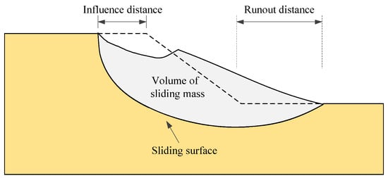
Figure 1. Large deformation characteristics of a slope.

2.1. Governing Equations of MPM

The MPM is a coupled Eulerian–Lagrangian approach that represents the continuum state using a set of Lagrangian particles while solving the governing equations on a fixed Eulerian background grid. This hybrid formulation effectively mitigates mesh distortion issues that commonly affect conventional grid-based numerical methods in large-deformation solid mechanics. The MPM governing equations for mass and momentum conservation can be expressed as follows:

$${\displaystyle \frac{\mathrm{d}\rho }{\mathrm{d}t}}+\rho \cdot \nabla \mathit{v}=0$$

(1)

$$\rho {\displaystyle \frac{\mathrm{d}\mathit{v}}{\mathrm{d}t}}=\nabla \cdot \mathit{\sigma }+\rho \mathit{b}$$

(2)

where $\rho$ is the current density, v is the velocity vector, $\mathit{\sigma }$ is the Cauchy stress tensor, and b is the body force vector, ∇(·) is the gradient operator, and t is the time. It is worth noting that Equations (1) and (2) assume the material is a continuum. In the MPM computational framework, it is not feasible to solve the governing equations directly. Instead, they must be transformed into a weak form and discretized into a finite set of particles. The numerical solution for the model’s state is then obtained by computing the motion state of each individual particle. In the whole domain Ω, the weak form of linear momentum is obtained by taking the virtual displacement $\delta \mathit{u}$ as an arbitrary test function and applying Green’s theorem:

$$\underset{\mathsf{\Omega }}{\int }\delta \mathit{u}\rho {\displaystyle \frac{\mathrm{d}\mathit{v}}{\mathrm{d}t}}\mathrm{d}\mathsf{\Omega }=-\underset{\mathsf{\Omega }}{\int }\nabla \left(\delta \mathit{u}\right)\sigma \mathrm{d}\mathsf{\Omega }+\underset{\mathsf{\Omega }}{\int }\delta \mathit{u}\rho \mathit{b}\mathrm{d}\mathsf{\Omega }+\underset{\mathrm{s}}{\int }\delta \mathit{u}\mathit{\tau }\mathrm{d}\mathrm{S}$$

(3)

where $\mathit{\tau }$ is the prescribed surface traction, and n is the outward unit normal of the body boundary surface S.

The computation process of the MPM is shown in Figure 2. The deformed body is discretized into particles, and Equation (3) is transformed into a particle integral. Thus, the mass density is defined as follows:

$$\rho \left({\mathit{x}}_i\right)=\sum _{p=1}^{n_p}{m}_p\delta \left({\mathit{x}}_i-{\mathit{x}}_p\right)$$

(4)

where m_p is the mass of particles, δ(·) is the Dirac delta function, and n_p is the total number of particles, ${\mathit{x}}_i$ and ${\mathit{x}}_p$ are the coordinates of mesh nodes and particles, respectively. Substituting Equation (4) into Equation (3), the integral form of the momentum equation can be written as follows:

$$\sum _{p=1}^{n_p}{m}_p{a}_i\delta {\mathit{u}}_{ip}+\sum _{p=1}^{n_p}{m}_p{\sigma }_p\delta {\mathit{u}}_{i,jp}-\sum _{p=1}^{n_p}{m}_p{\mathit{b}}_p\delta {\mathit{u}}_{ip}-\sum _{p=1}^{n_p}{m}_p{\mathit{\tau }}_p{h}^{-1}\delta {\mathit{u}}_{ip}=0$$

(5)

where ${\mathit{a}}_i$ is the acceleration vector of mesh nodes, and h represents the introduced fictitious boundary layer thickness.

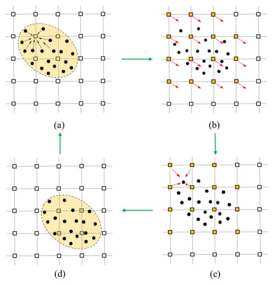
Figure 2. Illustrations of the computational process of MPM. (a) Particle to background mesh; (b) solution on the background mesh; (c) update particle; (d) mesh to particle. Red arrows represent physical quantity mapping calculations, and green arrows represent transformations of computational steps.

In Figure 2a, at the beginning of each time step, the mass and momentum of each particle are mapped onto the background mesh using the shape functions. To prevent dissipation of angular momentum, we adopt the Taylor Particle-In-Cell (TPIC) scheme proposed by Nakamura et al. [39], which is defined as follows:

$$m_i=\sum _{p=1}^{n_p}{S}_{ip}{m}_p$$

(6)

$${\mathit{p}}_i=\sum _{p=1}^{n_p}{S}_{ip}{m}_p\left[{\mathit{v}}_p+\nabla {\mathit{v}}_p\cdot \left({\mathit{x}}_i-{\mathit{x}}_p\right)\right]$$

(7)

$${\mathit{\nu }}_i={\displaystyle \frac{{\mathit{p}}_i}{m_i}}$$

(8)

where $m_i$ is the mass of the mesh nodes, $S_{ip}$ is the shape function. In the traditional MPM, the shape function is typically a linear interpolation function, which can cause discontinuities when particles cross element boundaries, leading to cell-crossing instabilities. In this study, a quadratic B-spline interpolation function is employed to mitigate such errors and enhance solution smoothness.

After the information of the particle is mapped onto the background mesh, the momentum equation can be simply expressed as follows:

$$m_i{\mathit{a}}_i={\mathit{f}}_i^{ext}+{\mathit{f}}_i^{int}$$

(9)

where ${\mathit{f}}_i^{ext}$ and ${\mathit{f}}_i^{int}$ are the external and internal forces at the mesh nodes, respectively, which are defined as:

$${\mathit{f}}_i^{ext}=\sum _{p=1}^{n_p}{S}_{ip}{m}_p{\mathit{b}}_p+\sum _{p=1}^{n_p}{S}_{ip}{\mathit{\tau }}_p{h}^{-1}{V}_p$$

(10)

$${\mathit{f}}_i^{int}=-\sum _{p=1}^{n_p}\nabla S_{ip}{\mathit{\sigma }}_p{V}_p$$

(11)

where $\nabla S_{ip}$ is the gradient of the shape function.

As shown in Figure 2b, Equation (9) is solved on the background mesh, and the current nodal velocities are obtained using the central difference method. The state variables of the particles (i.e., strain, stress, and velocity gradient) are then updated, where the particle velocity gradient ${\mathit{L}}_p$ is defined as follows:

$${\mathit{L}}_p^{t+1}=\sum _{i=1}^{n_n}\nabla S_{ip}{\mathit{v}}_i^{t+1}$$

(12)

where $n_n$ is the number of nodes, ${\mathit{v}}_i^{t+1}$ is the updated velocity vector at node i. This study focuses on simulating large-deformation slope failure.

According to Hooke’s law, the relationship between the stress increment Δσ and the strain increment Δε can be expressed as follows:

$$\Delta \mathit{\sigma }={\mathit{D}}^e\Delta {\mathit{\epsilon }}^{\mathit{e}}={\mathit{D}}^e\left(\Delta \mathit{\epsilon }-\Delta {\mathit{\epsilon }}^p\right)$$

(13)

where ${\mathit{D}}^e$ is the elastic stiffness matrix of the material, $\Delta {\mathit{\epsilon }}^p$ is the plastic strain increment. According to the plastic potential rule:

$$\Delta {\mathit{\epsilon }}^p={\displaystyle \frac{\partial Q}{\partial \mathit{\sigma }}}$$

(14)

where Λ is the plastic multiplier, given by the following:

$$\mathrm{\Lambda }={\displaystyle \frac{\frac{\partial F}{\partial \mathit{\sigma }}{\mathit{D}}^e\Delta \mathit{\epsilon }}{-\frac{\partial F}{\partial \mathit{H}}\frac{\partial \mathit{H}}{\partial A}\frac{\partial Q}{\partial \mathit{\sigma }}+\frac{\partial F}{\partial \mathit{\sigma }}{\mathit{C}}^e\frac{\partial Q}{\partial \mathit{\sigma }}}}$$

(15)

here H is the hardening parameter, and A is a state variable. Substituting Equations (14) and (15) into Equation (13) yields the following:

$$\Delta \mathit{\sigma }=\left({\mathit{D}}^e-{\displaystyle \frac{{\mathit{D}}^e\frac{\partial Q}{\partial \mathit{\sigma }}\frac{\partial F}{\partial \mathit{\sigma }}{\mathit{D}}^e}{-\frac{\partial F}{\partial \mathit{H}}\frac{\partial \mathit{H}}{\partial A}\frac{\partial Q}{\partial \mathit{\sigma }}+\frac{\partial F}{\partial \mathit{\sigma }}{\mathit{D}}^e\frac{\partial Q}{\partial \mathit{\sigma }}}}\right)\Delta \mathit{\epsilon }$$

(16)

For elastoplastic materials, the material stiffness matrix ${\mathit{C}}^{ep}$ can be obtained:

$${\mathit{C}}^{ep}={\mathit{D}}^e-{\displaystyle \frac{{\mathit{D}}^e\frac{\partial Q}{\partial \mathit{\sigma }}\frac{\partial F}{\partial \mathit{\sigma }}{\mathit{D}}^e}{-\frac{\partial F}{\partial \mathit{H}}\frac{\partial \mathit{H}}{\partial A}\frac{\partial Q}{\partial \mathit{\sigma }}+\frac{\partial F}{\partial \mathit{\sigma }}{\mathit{D}}^e\frac{\partial Q}{\partial \mathit{\sigma }}}}$$

(17)

In numerical computations, the strain increment is defined as the derivative of the displacement increment with respect to coordinates:

$$\Delta \mathit{\epsilon }={\displaystyle \frac{1}{2}}\left[{\displaystyle \frac{\partial \mathit{u}}{\partial \mathit{x}}}+{\left({\displaystyle \frac{\partial \mathit{u}}{\partial \mathit{x}}}\right)}^T\right]$$

(18)

In this study, the strain increment is obtained by forward time integration of the velocity gradient:

$$\Delta \mathit{\epsilon }={\displaystyle \frac{1}{2}}\left[{\displaystyle \frac{\partial \mathit{v}}{\partial \mathit{x}}}+{\left({\displaystyle \frac{\partial \mathit{v}}{\partial \mathit{x}}}\right)}^T\right]\Delta t$$

(19)

Substituting Equation (12) into the above expression gives the strain increment for each particle:

$$\Delta {\mathit{\epsilon }}_p^{t+1}={\displaystyle \frac{1}{2}}[{\mathit{L}}_p^{t+1}+{\left({\mathit{L}}_p^{t+1}\right)}^T]\Delta t$$

(20)

The objective stress rate (i.e.,${\mathit{\sigma }}_p^{\nabla }={\mathit{\sigma }}_p-\Delta W_p\cdot {\mathit{\sigma }}_p+{\mathit{\sigma }}_p\cdot \Delta {\mathit{W}}_p$) is used to eliminate the numerical impact from the rigid body rotation on stress. The incremental Cauchy stress can be computed by integrating over time as follows:

$${\mathit{\sigma }}_p^{t+1}={\mathit{\sigma }}_p^t+C^{ep}\Delta {\mathit{ϵ}}^{t+1}+\Delta t\left({\mathit{W}}_p^{t+1}\cdot {\mathit{\sigma }}_p^t-{\mathit{\sigma }}_p^t\cdot {\mathit{W}}_p^{t+1}\right)$$

(21)

$${\mathit{W}}_p^{t+1}={\displaystyle \frac{1}{2}}\left[{\mathit{L}}_p^{t+1}-{\left({\mathit{L}}_p^{t+1}\right)}^T\right]$$

(22)

After solving the momentum Equation (9) on the background mesh, the updated nodal information is mapped back to the material points to update their positions and velocities. The particle velocity is then updated as follows:

$${\mathit{v}}_p^{t+1}=\alpha {\mathit{v}}_{\mathrm{P}\mathrm{I}\mathrm{C}}^{t+1}+\left(1-\alpha \right){\mathit{v}}_{\mathrm{F}\mathrm{L}\mathrm{I}\mathrm{P}}^{t+1}$$

(23)

$${\mathit{v}}_{PIC}^{t+1}=\Delta t\sum _{i=1}^n{S}_{ip}{\mathit{v}}_i^{t+1}$$

(24)

$${\mathit{v}}_{FLIP}^{t+1}={\mathit{v}}_p^t+\Delta t\sum _{i=1}^n{S}_{ip}{\mathit{a}}_i^{t+1}$$

(25)

where ${\mathit{v}}_{PIC}$ and ${\mathit{v}}_{FLIP}$ are the updated velocity vector of particles using the PIC and FLIP schemes, respectively. $\alpha$ represents the proportionate contribution from the updated velocity of PIC scheme.

As shown in Figure 2d, the positions of particle are updated based on the updated velocity of the nodes:

$${\mathit{x}}_p^{t+1}={\mathit{x}}_p^t+\Delta t\sum _{i=1}^n{S}_{ip}{\mathit{v}}_i^{t+1}$$

(26)

2.2. Constitutive Model

In this study, the mechanical behavior of geomaterials is characterized with the elastic-perfectly plastic Drucker–Prager (D-P) model [40]. The yield function of the DP model is expressed as follows:

$$f=\left\{\begin{array}{cc}{f}^s=\sqrt{J_2}+q_{\phi }{I}_m-k_{\phi }\hspace{0.17em}\hfill & \mathrm{if} I_m\le {\sigma }^t\hfill \\ f^t=I_m-{\sigma }^t\hfill & \mathrm{if} I_m>{\sigma }^t\hfill \end{array}\right.$$

(27)

where $J_2$ is the second invariant of the deviatoric stress tensor, $I_m$ is the mean stress and ${\sigma }^t$ is the tensile strength (${\sigma }^t$ is set to zero in this study). The constitutive parameters $q_{\phi }$ and $k_{\phi }$ can be calculated as follows:

$$q={\displaystyle \frac{3\tan \phi }{\sqrt{9+12{\tan }^2\phi }}},k={\displaystyle \frac{3c}{\sqrt{9+12{\tan }^2\phi }}}$$

(28)

where c and φ are the cohesion and internal friction, respectively. In accordance with the non-associated plastic flow assumption, the plastic potential function g is as follows:

$$g=\left\{\begin{array}{cc}{g}^s=\sqrt{J_2}+q_{\phi }{I}_m-k_{\phi }\hspace{0.17em}\hfill & \mathrm{if} I_m\le {\sigma }^t\hfill \\ g^t=I_m\hfill & \mathrm{if} I_m>{\sigma }^t\hfill \end{array}\right.$$

(29)

where the expression of $q_{\varphi }$ is consistent with that of $q_{\mathrm{\phi }}$ except that the dilatancy angle $\varphi$ is used instead of φ.

2.3. Random Field Method

The autocorrelation function is a key quantity for characterizing the spatial correlation of soil properties [6]. In this work, the single exponential (SNX) autocorrelation function is used, which is expressed as follows:

$$\rho \left(d_h,d_v\right)=\exp \left[-2\left({\displaystyle \frac{d_h}{l_h}}+{\displaystyle \frac{d_v}{l_v}}\right)\right]$$

(30)

where $d_h$ and $d_v$ are the distances between two spatial coordinates of points in horizontal and vertical directions, respectively. $l_h$ and $l_v$ are scales of fluctuation in horizontal and vertical directions.

Based on the autocorrelation function defined in Equation (24), the autocorrelation matrix ${\mathit{C}}_{\mathrm{N}\times \mathrm{N}}$ is symmetric matrix, can be written as follows:

$${\mathit{C}}_{N\times N}=\left[\begin{array}{cccc}1& \rho \left({\tau }_{x12},{\tau }_{y12}\right)& \dots & \rho \left({\tau }_{x1N},{\tau }_{y1N}\right)\\ \rho \left({\tau }_{x21},{\tau }_{y21}\right)& 1& \dots & \rho \left({\tau }_{x2N},{\tau }_{y2N}\right)\\ \dots & \dots & \dots & \dots \\ \rho \left({\tau }_{xN1,}{\tau }_{yN1}\right)& \rho \left({\tau }_{xN2,}{\tau }_{yN2}\right)& \dots & 1\end{array}\right]$$

(31)

Assuming there is cross-correlation coefficient between c and φ, denoted as $r_{c,\phi }$, we can construct a cross-correlation coefficient matrix to quantify the relationship between these two parameters. The cross-correlation matrix is a two-dimensional symmetric matrix, which is defined as follows:

$${\mathit{R}}_{c,\phi }=\left[\begin{array}{cc}{r}_{c,\phi }& 1\\ 1& r_{c,\phi }\end{array}\right]$$

(32)

The autocorrelation matrix ${\mathit{C}}_{\mathrm{N}\times \mathrm{N}}$ and the cross-correlation matrix ${\mathit{R}}_{c,\phi }$ are decomposed into the product of a lower triangular matrix and its transpose matrix using CMD. The Cholesky decomposition is as follows:

$${\mathit{C}}_{N\times N}={\mathit{L}}_1{\mathit{L}}_1^T$$

(33)

$${\mathit{R}}_{c,\phi }={\mathit{L}}_2{\mathit{L}}_2^T$$

(34)

where ${\mathit{L}}_1$ and ${\mathit{L}}_2$ are lower triangular matrices of ${\mathit{C}}_{N\times N}$ and ${\mathit{R}}_{c,\phi }$, respectively.

A stochastic sampling approach is employed to generate standard normally distributed sample matrices $\mathit{\xi }$ of dimension $N\times 2$. The corresponding standard normal random field is then obtained as follows:

$${\mathit{H}}_s={\mathit{L}}_1\mathit{\xi }{\mathit{L}}_2^T=\left[{\mathit{H}}_s^c,{\mathit{H}}_s^{\phi }\right]$$

(35)

where ${\mathit{H}}_s$ is a standard normal random field matrix, which includes the random field of cohesion ${\mathit{H}}_s^c$ and ${\mathit{H}}_s^{\phi }$ is internal friction. Under the assumption of an independent standard normal random field, the cohesion and internal friction angle may take non-physical (negative) values. To avoid this issue, both parameters are assumed in this study to follow a log-normal distribution, as expressed below:

$${\mathit{H}}_l^i=\exp \left[{\mu }_{\ln \left(i\right)}\mathit{\Lambda }+{\sigma }_{\ln \left(i\right)}{\mathit{H}}_s^i\right], i=c,\phi$$

(36)

$${\sigma }_{\ln \left(i\right)}=\sqrt{\ln \left(1+{\left({\sigma }_i/{\mu }_i\right)}^2\right)}$$

(37)

$${\mu }_{\ln \left(i\right)}=\ln {\mu }_i-{\sigma }_{\ln \left(i\right)}^2/2$$

(38)

where ${\mu }_{\mathrm{i}}$ and ${\sigma }_i$ represent the mean and standard deviation of the normal random variable i, respectively. ${\mu }_{\ln \left(i\right)}$ and ${\sigma }_{\ln \left(i\right)}$ represent the mean and standard deviation of the normal random variable $\mathrm{l}\mathrm{n}\left(i\right)$, respectively. $\mathbf{\Lambda }$ represents a matrix of dimensions, N × 1, in which all elements are equal to 1.

3. Workflow of Method

To overcome these challenges, the proposed framework incorporates a parallel optimization algorithm to accelerate the generation of random field samples and leverages the GPU parallel computing of the GeoTaichi MPM solver [41] to significantly enhance the computational efficiency of slope simulations. The overall workflow of the framework is illustrated in Figure 3, comprising three main stages:

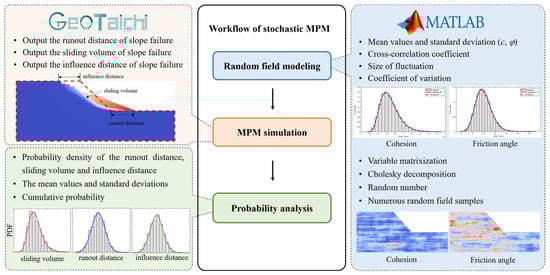
Figure 3. Workflow of stochastic MPM frame.

3.1. Random Field Generation

The generation of a random field is subdivided into three core phases: (1) the initial phase, (2) assembly and decomposition of the autocorrelation matrix, and (3) subsequent random field matrix operations.

Initial phase: First, the coordinate information of the background grid nodes occupied by the slope model is extracted. Then, the centroid coordinates of each element in the slope model are calculated based on the nodal coordinates. This approach aims to reduce the dimension of the autocorrelation matrix. For example, in the model, each element initially contains four particles. Calculating the autocorrelation matrix based on element centroid coordinates, compared to the method based on particle coordinates, can reduce memory consumption by a factor of four, thereby achieving a reduction in the dimension of the autocorrelation matrix.

Autocorrelation matrix assembly and decomposition: In this phase, the coordinates matrix of element centroids is subdivided into blocks. The autocorrelation matrix for each block is computed using highly parallelized processing. To mitigate communication bottlenecks inherent in data transfer, the global autocorrelation matrix is assembled using asynchronous data transfer protocols. The subsequent decomposition of the final autocorrelation matrix is also executed in a parallel algorithm.

Random field matrix operations: The computation of the standard random field matrix, governed by Equation (35), involves matrix L1 and the sample matrices ξ. In models with a high particle count, the dimensions of these matrices become exceedingly large. The traditional serial algorithm is extremely time-consuming when performing vector multiplication calculations. To overcome this problem, the pagetimes function is used to perform batched matrix multiplications on the vectorized matrices, resulting in a substantial increase in computational efficiency.

Finally, a nodal averaging algorithm [42] is employed to map the soil parameter information from the element centers to each material point, as shown in Figure 4, thereby obtaining a material point-based random field model.

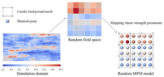
Figure 4. Schematic diagram of the mapping of the spatial variables with the random field elements and material points.

3.2. MPM Simulation and Data Extraction

A GPU-accelerated MPM solver is used to efficiently perform batch simulations of slope models with the generated random fields. To reduce particle cell-crossing errors, quadratic B-spline basis functions are employed. Post-processing is carried out using custom Python 3.10 version scripts within ParaView 5.9.1 version to extract large-deformation landslide behavior data for subsequent probabilistic analysis.

3.3. Probabilistic Statistical Analysis

The collected large deformation behavior data are statistically analyzed to reveal the underlying influence of spatial variability in soil properties on landslide behavior. These analyses provide scientific evidence for slope stability assessment and landslide risk management. All numerical simulations are conducted on a workstation equipped with an Intel Xeon Gold 6238 CPU, NVIDIA GEFORCE RTX 5000 GPU, 256 GB RAM, and a Windows operating system.

4. Validation of Proposed Method

The validation of the computation framework comprises two components: the validation of geotechnical random field generation and the MPM solver.

4.1. Validation of Random Field Method

To validate the applicability of the random field method used in this study, a stratigraphic model was constructed with the dimensions shown in Figure 5. The model has a height of 20 m and a width of 50 m and is discretized into 4000 grid cells and 16,000 particles. The soil properties and corresponding statistical parameters are listed in Table 1. Three grid-center locations are selected as monitoring points: A (24.75, 9.75), B (24.75, 19.75), and C (24.75, 0.25). Using the CMD approach, 10,000 random field realizations for both cohesion and internal friction angle are generated, and the values at the monitoring points are subsequently analyzed to verify the accuracy of the proposed method.

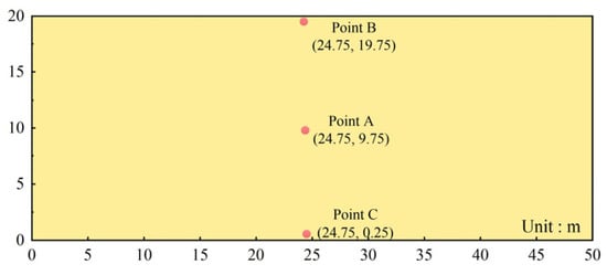
Figure 5. Stratigraphic model for the validation of the random field theory.

Figure 6a illustrates a typical spatial distribution of the random field for cohesion, which exhibits clear position-dependent variability. Figure 6b–d show the probability density functions (PDFs) of cohesion at monitoring points A, B, and C, respectively. The blue curves represent log-normal distribution functions defined by the mean and standard deviation listed in Table 2, while the red curves are fitted to the sampled random field data. The close agreement between the fitted PDFs and the theoretical log-normal distributions at all three points confirms that the autocorrelation structure of the cohesion random field is well preserved.

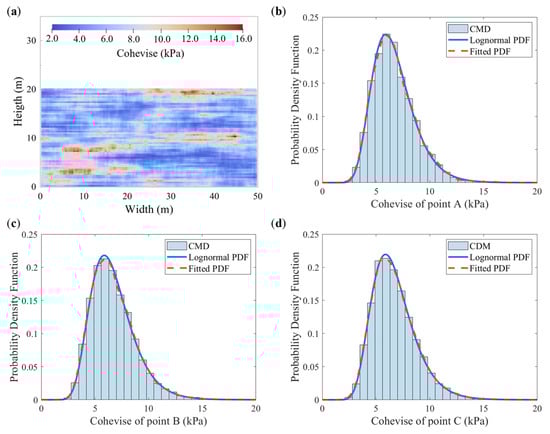
Figure 6. Cohesion random field sample illustration and prescribed probability density functions. (a) Sample example of a cohesion random field; (b) point A; (c) point B; (d) point C.

Table 2. Soil parameters for the validation of the random field method.

Parameter	Mean Value, μ	COV	Fluctuation Length, lh and lv (m)	Cross-Correlation Coefficient	Probability Distribution
Cohesion	6.7 kPa	0.3	20, 2	−0.5	Log-normal
Friction angle	20°	0.2			Log-normal

Figure 7a shows the spatial distribution of the internal friction angle for the same random field sample presented in Figure 6, which also demonstrates pronounced spatial variability. Figure 7b–d display the probability density functions (PDFs) of the internal friction angle at monitoring points A, B, and C, respectively. The blue curves represent log-normal distributions defined by the mean and standard deviation provided in Table 2, while the red curves correspond to fitted distributions based on the random field sample data. The close agreement between the fitted PDFs and the theoretical log-normal curves validates that the autocorrelation structure of the internal friction angle field is well preserved.

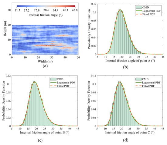
Figure 7. Friction angle random field sample illustration, monitoring point histograms, and prescribed probability density functions. (a) Sample example of a friction angle random field; (b) point A; (c) point B; (d) point C.

Furthermore, the distribution in Figure 7a exhibits a clear negative correlation with the cohesion distribution in Figure 6a; regions of higher cohesion correspond to lower internal friction angles, and vice versa. This observation aligns with the predefined cross-correlation coefficient of −0.5 between the two parameters, confirming that the proposed random field approach effectively captures the interdependence between cohesion and internal friction angle.

The Kolmogorov–Smirnov (KS) test [43] is employed to evaluate whether the model predictions follow a log-normal distribution. In this test, the p-value represents the probability of obtaining the current sample, or a more extreme one, under the assumption that the hypothesis is true. Table 3 presents the p-values obtained from the KS test at different points. All p-values substantially exceed the 0.05 significance threshold, indicating that the generated sample data are consistent with a log-normal distribution.

Table 3. The obtained p-values of different points with the KS test.

Parameters	Point A	Point B	Point C
Cohesion	0.685	0.398	0.722
Friction angle	0.876	0.864	0.797

To quantify the accuracy of the proposed random field method, a verification framework employing three statistical metrics (such as the coefficient of determination (R²), absolute error, and root mean square error (RMSE)) was implemented. Table 4 and Table 5 show that three metrics are used to quantitatively assess the agreement between the model predictions and theoretical expectations. The obtained R² values all exceed 0.997, indicating that the random field method explains more than 99.7% of the variance in the observed data. Absolute errors remain consistently low (below 0.0022), reflecting minimal deviation between the predicted and theoretical distributions. Furthermore, the root mean square error is below 0.0037 across all measurement points, confirming the high predictive accuracy of the method. Collectively, these statistical results demonstrate that the predictions generated by the random field method are in excellent agreement with theoretical benchmarks, thereby validating its high accuracy and reliability.

Table 4. Validation of the random field method for cohesion.

Cohesion	R2	Absolute Errors	RMSE
Point A	0.9983	0.001656	0.002842
Point B	0.9973	0.002133	0.003671
Point C	0.9988	0.001522	0.002429

Table 5. Validation of the random field method for the friction angle.

Friction Angle	R2	Absolute Errors	RMSE
Point A	0.9991	0.000690	0.001090
Point B	0.9989	0.000808	0.001238
Point C	0.9983	0.001032	0.001554

4.2. Validation of MPM

This section presents a simulation of column collapse, with model accuracy verified through comparison to experimental results reported by Nguyen et al. [44], using identical material properties: elastic modulus of E = 5.84 MPa, Poisson’s ratio of μ = 0.3, density ρ = 2040 kg/m³, friction angle φ = 21.9°, and a cohesion of c = 0.0 kPa for the column of aluminum rods. The collapse behavior of the column under gravity was simulated using the MPM. In the model, the base is fully constrained, while horizontal movement on the right boundary is restricted.

The experimental and numerical results are compared in Figure 8. The stable state of the column in the experiment is shown in Figure 8a. The MPM simulation successfully reproduced the free-surface profile of the column, and the predicted distribution of stable regions showed excellent agreement with experimental observations (Figure 8b). The experimental result shows a sliding distance of 30 cm, while the simulated data is 28.4 cm, with a relative error of only 5.3% between them. This comparison confirms that the employed MPM solver can accurately capture the behavior of granular soil materials under large deformation conditions.

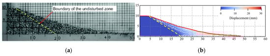
Figure 8. Final state of column (a) experiment result (b) simulation result. The red line represents the final outer surface profile of the granular pile in the experiment, while the yellow line indicates the boundary of the undisturbed region.

4.3. Deterministic Analysis of Large Deformation of Slope

This section examines the large-deformation behavior of a slope simulated using the GPU-accelerated MPM model, along with a computational efficiency analysis to further optimize performance. The slope geometry consists of a height of 20 m, a length of 50 m, and an inclination of 45° to the horizontal. The model boundaries are fully constrained at the base, while horizontal displacements are restricted along both lateral sides, as shown in Figure 9. This study focuses on slope failure under self-weight, which belongs to a quasi-static problem. The fixed boundaries effectively can prevent rigid body motion and are widely used and accepted in the literature [31,37,40]. Soil properties are listed in Table 6. In line with the study’s focus on large-deformation behavior, only simulation cases exhibiting landslide displacements greater than 0.4 m are included in the analysis dataset to minimize the influence of minor deformations on the results.

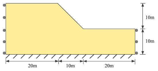
Figure 9. Geometry of a slope.

Table 6. Soil properties for deterministic analysis.

Parameters	Unit	Value
Soil weight, γ	kN/m3	2000.0
Elastic modulus, E	MPa	100.0
Poisson’s ratio, ν		0.3
Cohesion, c	kPa	6.7
Friction angle, φ	°	20.0
Dilatancy angle, ψ	°	0.0

Figure 10 presents the initial stress distribution and the final displacement field from the deterministic slope analysis. The simulation procedure consisted of two sequential steps. First, the initial stress state of the slope model was computed using an elastic constitutive relationship. Subsequently, the large-deformation behavior of the slope under self-weight conditions was analyzed with the Drucker–Prager constitutive model. As shown in Figure 10b, post-failure motion ceased at approximately 8 s, yielding a runout distance of 6.10 m, an influence distance of 6.26 m, and a sliding mass volume of 56.76 m². The latter was computed by multiplying the number of moving particles (displacement greater than 0.4 m) by the volume of each particle.

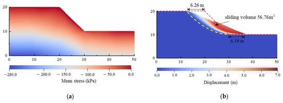
Figure 10. Initial and final state of slope by deterministic analysis: (a) mean stress field at initial state; (b) displacement field at final state.

The appropriate selection of simulation time is crucial for achieving computational efficiency in landslide analyses. Figure 11 shows the temporal evolution of the slope’s large-deformation characteristics. Both the runout distance and the influence distance increase rapidly during the initial stages and then progressively slow, with the runout distance continuing to grow slightly over time. The deformation characteristics stabilize at approximately 4.6 s. To ensure numerical stability and consistency across all cases, the simulation duration for each random field realization is conservatively set to 8 s in this study. The convergence of the large-deformation response was determined based on the decay of the system’s total kinetic energy [45]. Specifically, the deformation is considered to have stabilized when the kinetic energy diminishes and remains below a specified threshold (e.g., 1% of its peak value), indicating a quasi-static state. As shown in Figure 11b, this criterion is met at 4.6 s, after which the kinetic energy plateaus at a negligible level. Furthermore, the influence of floating-point precision on the simulation results of slope failure involving large deformations in the GPU-accelerated MPM is discussed, with a comparative analysis provided in the first case of Appendix A.

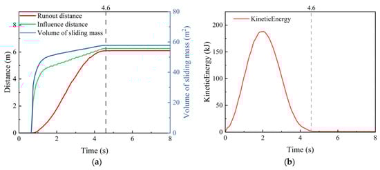
Figure 11. Variation curve of the slope failure response. (a) Variation in the large deformation characteristics of the slope, (b) variation in kinetic energy with large deformation of the slope.

To examine the effect of background mesh size on the large-deformation behavior of slopes and the associated computational time, five mesh sizes—0.125 × 0.125 m, 0.2 × 0.2 m, 0.25 × 0.25 m, 0.5 × 0.5 m, and 1.0 × 1.0 m—were used to discretize the slope model, while the incremental time size Δt can be obtained by the Courant condition.

$$\Delta t=\mathrm{C}\mathrm{F}\mathrm{L}{·L}_e·\sqrt{{\displaystyle \frac{\rho \left(1+v\right)\left(1-2v\right)}{E\left(1-v\right)}}}$$

(39)

where L_e is the size of the mesh, ρ is the density, ν is Poisson’s ratio, E is the Young’s modulus, and CFL is the Courant-Friedrichs-Lewy Constant. The incremental times corresponding to the grid sizes of each model are shown in Table 7. To ensure the objectivity of the comparison of computational efficiency and keep the incremental step size consistent, the incremental time was unified as 3 × 10⁻⁴ s.

Table 7. The incremental times corresponding to the grid sizes of each model by the Courant condition.

Background Mesh Size (m)	0.125	0.2	0.25	0.5	1.0
Incremental time size (s)	4.82 × 10−4	7.71 × 10−4	9.64 × 10−4	1.93 × 10−3	3.85 × 10−3

As shown in Figure 12a, both runout distance and influence distance increase as the mesh size decreases below 0.25 m. Convergence is essentially reached for mesh sizes of 0.20 m and 0.125 m. However, the corresponding computational times are 58.71 s and 93.25 s, respectively, as illustrated in Figure 12b. Considering the substantial savings in runtime with minimal loss of accuracy, a mesh size of 0.20 m is adopted for the subsequent probabilistic analyses. Figure 13 illustrates the variation in runout distance and influence distance when the mesh size is 0.2 m. As the time increment step size decreases, the stable value of the runout distance exhibits minor fluctuations but generally stabilizes overall, while the impact of this variation on the influence distance remains relatively limited.

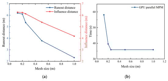
Figure 12. The impact of background mesh size. (a) The runout and influence distance with mesh size, and (b) the computational time with mesh size.

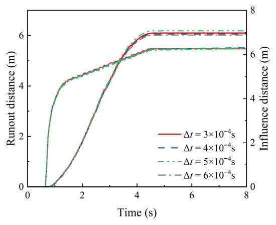
Figure 13. The variation in runout and influence distance with time during slope failure.

4.4. Computational Efficiency

Monte Carlo analysis of landslide deformation characteristics typically requires 10³ to 10⁶ realizations to obtain stable statistical results, which presents significant computational challenges for both random field sample generation and MPM simulations. In this study, the efficiency of the proposed parallelization strategy is verified; we generated 1500 random field samples for the slope model shown in Figure 9. Figure 14a compares the computation times of the serial and parallel algorithms of random field generation. Across all cases, the serial method required substantially longer runtime than the parallel approach. For instance, with 3020 particles, the serial computation time was 6.48 s compared with only 0.11 s for the parallel method; for 75,100 particles, the serial execution took 52.68 min, whereas the parallel computation required just 0.44 min, a speedup of approximately 120×. These results clearly demonstrate that the optimized parallel algorithm dramatically improves the efficiency of random field sample generation.

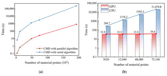
Figure 14. Random field MPM computation time. (a) Time of random field sample generation, and (b) MPM computation time.

To further reduce computation time, a GPU-parallel-accelerated MPM solver is employed for landslide modeling. The slope model described in Section 4.3 is computed using both CPU-based and GPU-based MPM solvers for comparison. Figure 14b presents the computation time for varying particle counts. As the number of particles increases, the runtime of the CPU-based MPM [46] rises sharply, whereas the GPU-based MPM exhibits minimal fluctuation and remains relatively stable. For small particle counts, the computational load is insufficient to fully exploit the GPU’s processing capacity; however, the performance gains achieved with the GPU-based approach remain significant. At 75,100 particles, the GPU solver is 532 times faster than the CPU solver, reducing computation time by approximately 5.8 h per single run. Given that this study required 1500 realizations per variable, amounting to a total of 19,500 random field samples, the aggregate time savings from GPU acceleration are substantial.

By integrating CMD with a parallelized sample-generation algorithm and the GPU-accelerated MPM solver, the proposed stochastic field simulation framework achieves exceptional computational efficiency, enabling large-scale Monte Carlo analyses to be conducted within practical timeframes.

5. Probabilistic Analysis and Discussions

In this section, the random field MPM is employed to investigate the post-failure behavior of the slope model (Figure 9) arising from the spatial variability of soil parameters, namely cohesion and internal friction angle. This approach integrates MPM with random field theory within an MCS framework. Uncertainty analyses using MCSs typically require 10³–10⁶ simulations to obtain statistically reliable results. While a higher number of simulations can improve accuracy, it also significantly increases computational cost.

To determine an adequate sample size for statistical convergence, a representative case of non-deterministic large-deformation slope analysis is examined, with the statistical properties of soil parameters provided in Table 2. It is important to note that the soil parameters used in all models in this section are listed in Table 6. For the deterministic models, the soil strength parameters (cohesion and friction angle) were assigned the mean values of their corresponding random fields. Figure 15 shows the convergence behavior of the mean and standard deviation for the large-deformation indicators (runout distance, influence distance, and volume of sliding mass) as the number of random field samples increases. A total of 1500 spatially variable random field realizations are generated and analyzed. At low sample counts, both the mean and standard deviation of post-failure metrics fluctuate substantially. Stabilization occurs beyond approximately 620 simulations. Based on this observation, the MCS sample size is set to 1500 per case in this study to ensure statistical convergence.

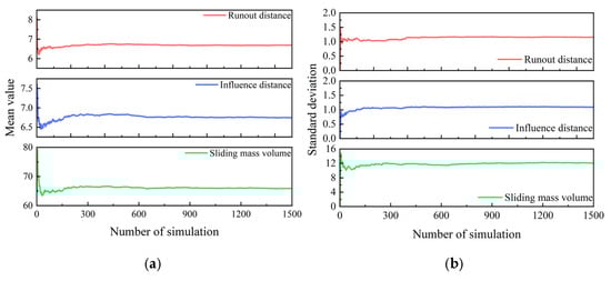
Figure 15. The convergence of MCSs: (a) mean value of slope post-failure behavior with the number of simulations; (b) standard deviation of slope post-failure behavior with the number of simulations.

5.1. The Influence of Horizontal Fluctuation Scale

To clearly demonstrate the influence of the horizontal fluctuation scale on the post-failure behavior of the slope, five cases with different horizontal fluctuation scales (l_h = 2, 4, 6, 8, 10 m) are analyzed, while all other computational parameters are as listed in Table 2 and Table 6. For each fluctuation scale, 1500 random field realizations are generated and modeled.

Figure 16a shows the probability density histogram of runout distance obtained from the MCS analysis for the case with horizontal anisotropy (l_h = 10.0 m). The data are fitted with both normal (red line) and log-normal (blue line) distribution functions. Comparison with the histogram and probability density curves indicates that the normal distribution provides a better fit. The KS goodness-of-fit test further confirms that, at the 5% significance level, the runout distances in all cases are well represented by a normal distribution. Figure 16b shows the normal distribution probability density curves for runout distances with different horizontal fluctuation scales. In addition, the runout distances corresponding to both the 1–99% and 25–75% quantile ranges increase with horizontal fluctuation length. A comparative analysis of the five anisotropic cases reveals that in each case, more than 70% of the simulated values exceed the deterministic runout distance of 6.10 m. This finding suggests that deterministic analysis may underestimate failure risk, highlighting the importance of incorporating spatial heterogeneity of soil properties in landslide hazard assessments.

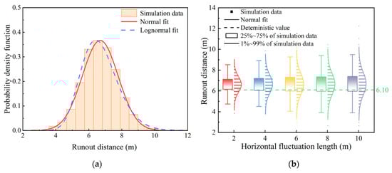
Figure 16. Histogram, probability density functions, and box diagram of the runout distance under different l_h. (a) l_h = 10.0 m; (b) effect of l_h on the box diagram.

Figure 17a shows the probability distribution variations in influence distance with horizontal anisotropy (l_h = 10.0 m). It can be seen that the normal distribution probability density function is a better fit to the histogram of the influence distance, which is mostly in the range of 5.97–7.50 m, and the maximum runout distance can reach up to 10.28 m; the mean value is 6.70 m, in contrast to 6.26 m as determined by deterministic analysis. This discrepancy might result in an underestimation of the potential risk to buildings situated near the top of the slope. The normal distribution probability density curves for l_h values of 2.0, 4.0, 6.0, 8.0, and 10.0 m are shown in Figure 17b. The range of influence distance within the 25–75% intervals rises and expands with the increasing horizontal fluctuation scale.

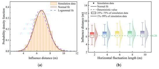
Figure 17. Histogram, probability density functions, and box diagram of the influence distance under different l_h values. (a) l_h = 10.0 m; (b) Effect of l_h on the box diagram.

Figure 18a presents the histogram and probability distribution of sliding mass volume for the case with horizontal anisotropy (l_h = 10.0 m). Unlike the two deformation characteristics analyzed previously, the volume distribution aligns more closely with a log-normal distribution, consistent with findings obtained using the SPH method [47]. Most values fall within the range of 56.00–72.84 m², with a mean volume of 66.65 m² exceeding the 57.76 m² obtained from deterministic analysis.

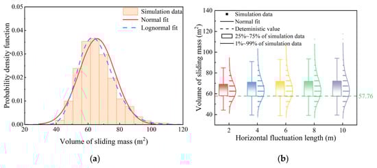
Figure 18. Histogram, probability density functions, and box diagram of the volume of sliding mass under different l_h. (a) l_h = 10.0 m; (b) the effect of l_h on the box diagram.

Figure 18b shows the box plots and corresponding log-normal probability density functions for cases with l_h = 2 m, 4 m, 6 m, 8 m, and 10 m. Comparative analysis reveals that in all five cases, more than half of the simulated volumes exceeded the deterministic result, accounting for 80.46%, 76.88%, 74.66%, 74.07%, and 73.53% of the realizations, respectively. These findings indicate that deterministic analysis may systematically underestimate sliding volumes, potentially leading to non-conservative and unsafe risk assessments for infrastructure located near the slope. It is worth noting that the large deformation data of the slope models in all cases have been validated by the KS goodness-of-fit test, with p-values significantly above the critical threshold at the 5% significance level.

Figure 19 illustrates the variation in the mean and standard deviation of the large-deformation characteristics with changes in the horizontal fluctuation scale. As the fluctuation scale increases, both the mean and standard deviation of the influence distance and the sliding mass volume show a gradual upward trend. In contrast, the mean runout distance fluctuates but exhibits an overall slow increase.

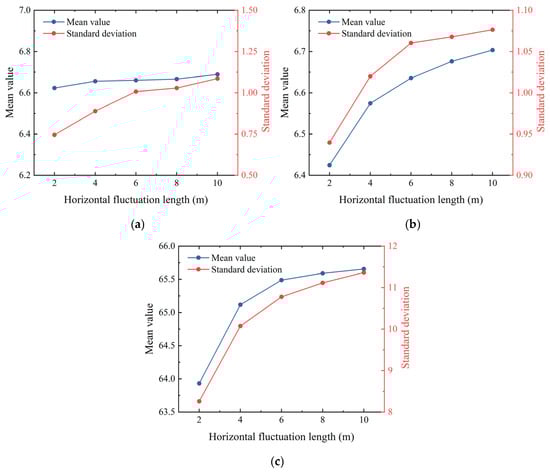
Figure 19. The variation in the mean and standard deviation of the large deformation characteristics. (a) Runout distance; (b) influence distance; (c) volume of sliding mass.

The preceding analysis indicates that the horizontal fluctuation scale significantly affects the large-deformation characteristics of landslides. In heterogeneous slopes, shear bands tend to develop within zones of lower soil shear strength [48]. When the horizontal fluctuation scale is small, it is easier for failure paths to traverse continuous weak soil zones. As a result, the distribution of deformation characteristics becomes relatively concentrated, yielding a lower standard deviation in the statistical results. Conversely, as the fluctuation scale increases, localized regions of higher soil strength appear within the slope. These stronger zones may force shear bands to deviate or prevent them from propagating continuously, producing a more dispersed distribution of deformation characteristics and, consequently, larger standard deviations.

5.2. The Influence of Coefficient of Variation

This subsection investigates the influence of the COV of cohesion and internal friction angle on the large-deformation characteristics of slopes modeled with random fields. All other parameters remain as given in Table 6, while the COV values for cohesion and internal friction angle are varied across five cases, as listed in Table 8.

Table 8. Soil properties for uncertainty analysis.

Parameter	Case 1	Case 2	Case 3	Case 4	Case 5
COVc	0.2	0.25	0.3	0.35	0.4
COVφ	0.1	0.15	0.2	0.25	0.3

Figure 20a–c present the probability density functions (PDFs) and box plots for the large-deformation characteristics of the slope samples. The runout distance and influence distance follow a normal distribution, whereas the sliding volume conforms more closely to a log-normal distribution. With increasing COV_c,φ, the spread of the results widens across both the 1–99% and 25–75% quantile ranges. Simultaneously, the proportion of slopes with large-deformation characteristics exceeding the deterministic analysis results increases markedly. Higher COV_c and COV_φ values result in broader, flatter, and more skewed probability distributions, indicating that the post-failure behavior of landslides exhibits more extreme outcomes, with deformation characteristics showing either substantially greater or considerably smaller values.

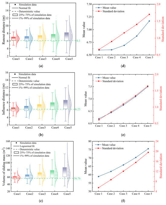
Figure 20. Probability density function, box diagram, and cumulative density function of the large deformation characteristics of the slope under different COVs. (a–c) Probability density function, box diagram, and cumulative density function of the runout distance, influence distance, and the volume of sliding mass; (d–f) the mean value and standard deviation of the runout distance, influence distance, and the volume of sliding mass.

Figure 20d–f show the variation in the mean and standard deviation of the large-deformation characteristics with changes in COV_c,φ. As COV_c,φ increases, both the mean and standard deviation of the runout distance, influence distance, and sliding mass volume rise, demonstrating a positive correlation between the uncertainty in large-deformation characteristics and the COV_c,φ of shear strength parameters.

To further illustrate the influence of COV_c,φ on the large-deformation characteristics of the slope, two representative simulation results are selected for detailed analysis: Case 1 (COV_c = 0.2, COV_φ = 0.1) and Case 5 (COV_c = 0.4, COV_φ = 0.3). Previous studies [31,38] have shown that spatial fluctuations in shear strength parameters become more pronounced with increasing COV_c,φ. Figure 21(a1–a3,b1–b3) confirm this trend, as the distribution of shear strength parameters in Case 5 (higher COV_c,φ) exhibits considerably greater dispersion compared to Case 1. This enhanced variability results in higher uncertainty in the large-deformation response and a larger standard deviation in the statistical outcomes.

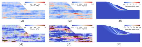
Figure 21. Two typical examples of random fields. (a1) Cohesion field of case 1; (a2) friction angle field of case 1; (a3) equivalent plastic strain field of case 1; (b1) cohesion field of case 5; (b2) friction angle field of case 5; (b3) equivalent plastic strain field of case 5.

When low-strength zones are located near the potential sliding surface, the post-failure behavior of the landslide becomes more violent and complex, as illustrated in Figure 21(a3,b3). This effect is primarily reflected in the increased mean values and standard deviations of the statistical distributions of the slope’s large-deformation characteristics.

5.3. The Influence of the Cross Correlation Coefficient

To examine the influence of the correlation between cohesion and internal friction angle on the post-failure behavior of slopes, five different cross-correlation coefficients (R_c,φ = −0.5, −0.25, 0.0, 0.25, 0.5) were adopted to generate random field samples, consistent with previous studies [49,50]. All other computational parameters were taken from Table 6. To ensure statistical stability, the proposed computational framework was used to generate and analyze 1500 random field realizations for each case.

Figure 22a–c depict the statistical distributions of runout distance, influence distance, and sliding volume. The first two parameters follow normal distributions, whereas the sliding volume is better described by a log-normal distribution. As the correlation coefficient between cohesion and internal friction angle increases, the corresponding probability density curves progressively broaden, flatten, and shift rightward. In all cases, the mean values exceed those obtained from deterministic analysis, suggesting that relying solely on deterministic results may significantly underestimate failure risk. To further verify this finding, a series of simulations with varying soil cohesion values were conducted for the large-deformation slope failure analysis. The results consistently demonstrate that the deterministic approach systematically underestimates the landslide risk. The comparative data from these parametric studies are presented in the second case of Appendix A.

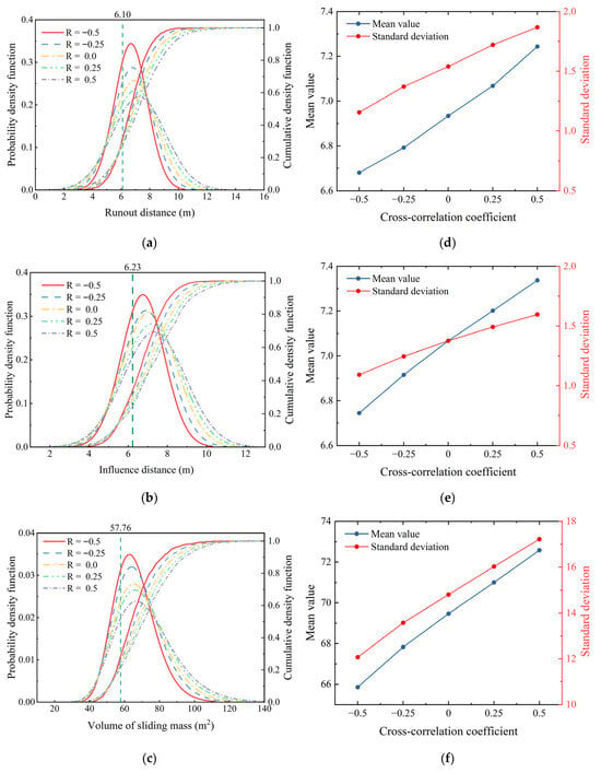
Figure 22. Probability density function, cumulative density function and the variation of mean value and standard deviation of the large deformation characteristics of slope under different cross correlation coefficient. (a–c) The probability density function and cumulative density function of the runout distance, influence distance and the volume of sliding mass; (d–f) The mean value and standard deviation of the runout distance, influence distance and the volume of sliding mass.

Figure 22d–f further show that both the mean and standard deviation of all large-deformation characteristics increase consistently with higher positive correlation. This trend can be explained by the fact that, under negative (R < 0) or zero (R = 0) correlation, spatial variability in shear strength is effectively moderated: zones of low cohesion (c) or low friction angle (φ) tend to be adjacent to zones of higher strength (high c or high φ), which provide additional confinement and reduce the continuous development of slip bands. In contrast, a stronger positive correlation diminishes these compensating strength patterns, allowing shear bands to propagate more freely and thereby increasing both the extent and variability of large-deformation responses.

Figure 23(a1–a5,b1–b5) show the distributions of cohesion and internal friction angle for five representative specimens under different cross-correlation coefficients. While the cohesion distribution remains essentially unchanged, the internal friction angle distribution varies noticeably. This difference arises from the use of identical random seeds to generate the samples, thereby minimizing interference from other stochastic factors.

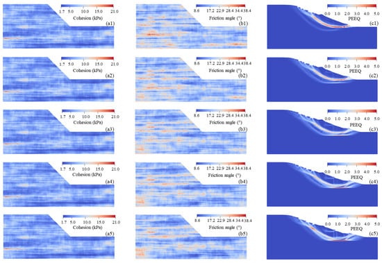
Figure 23. Typical realizations of random fields of cohesion, friction angle, and equivalent plastic strain fields. (a1–c1) Random field of cohesion, friction angle, and equivalent plastic strain fields with R _c,φ = −0.5, (a2–c2) Random field of cohesion, friction angle, and equivalent plastic strain fields with R _c,φ = −0.25, (a3–c3) Random field of cohesion, friction angle, and equivalent plastic strain fields with R _c,φ = 0.0, (a4–c4) Random field of cohesion, friction angle, and equivalent plastic strain fields with R _c,φ = 0.25, (a5–c5) Random field of cohesion, friction angle, and equivalent plastic strain fields with R _c,φ = 0.5.

Figure 23c1 reveals that the primary shear band extends from the slope toe to the crest. When the cohesion at the slope toe is low, an increase in R_c,φ leads to a downward shift in the shear band, accompanied by an expansion of the affected area and landslide volume. This phenomenon indicates that under conditions of low cohesion at the slope toe, a stronger positive correlation induces a systematic reduction in the internal friction angle at corresponding locations (Figure 23(b1–b5)), thereby forming a persistently weak path. This mechanism renders the slope more susceptible to large-deformation failure along the critical potential slip surface. In contrast, when the cohesion at the slope toe is high, an increase in R_c,φ results in an elevation of the internal friction angle at the toe, which effectively suppresses slope deformation. As illustrated in Figure 22a–c, both the mean and standard deviation of the large-deformation characteristics of the slope exhibit a significant increase with rising R_c,φ. This trend demonstrates that the proposed framework effectively captures the elevated risk associated with positive correlation, underscoring its robustness in probabilistic landslide assessment.

5.4. Hazard Zoning of Landslides

The proposed framework enables a practical hazard zonation analysis for common structures located at the slope crest or toe that are susceptible to post-failure landslide impacts. To reduce the impact of landslide disasters. To reduce the impact of landslide disasters, it is very necessary to classify the potential disaster levels. We adopted the event likelihood classification method proposed by Lacasse and Nadim [37] and computed the exceedance probabilities for large-deformation characteristics (i.e., runout distance R and influence distance I) of the random field slope. A limit state function G can be written as follows:

$$G_R=R_T-R$$

(40)

$$G_R=I_T-I$$

(41)

where R_T and I_T are the threshold values of the runout and influence distance for the landslide. When G is less than zero, the runout and influence distance exceed the threshold values. The exceedance probability function P of the runout and influence distance for the landslide can be formulated as follows:

$$P\left(R>R_T\right)=P\left[G_R\left(r\right)\le 0\right]={\int }_{G_R\left(r\right)\le 0}{f}_r\left(r\right)\mathrm{d}r$$

(42)

$$P\left(I>I_T\right)=P\left[G_I\left(i\right)\le 0\right]={\int }_{G_I\left(i\right)\le 0}{g}_i\left(i\right)\mathrm{d}i$$

(43)

where the f_r(r) is the corresponding joint probability density function of the runout distance, g_i(i) is the corresponding joint probability density function of the influence distance. Classification of potential landslide hazard levels is achieved through the exceedance probability of the slope’s deformation characteristics.

A set of parameters was adopted for the instance analysis of spatial variability: COVs for soil cohesion and internal friction angle of 0.3 and 0.2, respectively, a horizontal fluctuation scale of 20, a vertical fluctuation scale of 2, and R_c,φ between the two parameters varying across −0.5, −0.25, 0.0, 0.25, and 0.5. Figure 24 illustrates the exceedance probability curves for the landslide runout and influence distance corresponding to the random field slope. The figure simultaneously highlights the potential hazard zones based on the classification standards. Each curve approximately represents the exceedance probability of the landslide failure impacting structures at different distances from the slope crest (I_s) or slope toe (R_s). The results indicate that the probability P (I > I_s) decreases with increasing distance from the crest, and P (R > R_s) decreases with increasing distance from the toe. Notably, the slope failure tends to form a wider influence zone and constitute a higher hazard level when the soil cohesion and internal friction angle exhibit a positive correlation, which is evidenced by the higher exceedance probabilities observed at the same I_s or R_s distances.

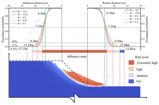
Figure 24. Illustration of the influence zone associated with exceedance probability in the partial slope model.

Considering R_c,φ = 0.5 as the most unfavorable scenario, the risk areas are delineated based on exceedance probabilities of 50%, 10%, 1%, and 0.1%. Regions where I_s < 7.33 m and R_s < 7.21 m are classified as the extreme hazard zone. Subsequently, as the exceedance probabilities P(I > I_s) and P(R > R_s) decrease from 50% to 10%, the hazard zone transitions to the high hazard zone (light-shaded area in Figure 24), covering the distance ranges 7.33 m < I_s < 9.28 m and 7.21 m < R_s < 9.59 m. In this most unfavorable case, distances of I_s = 11.25 m and R_s = 12.08 m are established as the boundary separating the medium- and low-risk zones (corresponding to an approximate 1% exceedance probability).

This study validates that the integration of the proposed random field MPM framework with probabilistic statistics enables the quantitative assessment of post-failure influence zones. By explicitly accounting for the spatial variability of soil parameters, the method effectively overcomes the limitation of traditional deterministic analyses, which may severely underestimate the large-deformation failure impact area, thereby providing a more accurate assessment of the threat posed to human life and infrastructure. Furthermore, on an engineering practice level, this quantitative assessment offers a more rigorous and reliable basis for building planning and disaster mitigation decisions in slope-adjacent areas compared to conventional deterministic approaches.

6. Conclusions

This study establishes a high-performance stochastic computational framework designed to quantify the impact of spatial variability on large-deformation slope failures. To address the significant computational costs associated with traditional probabilistic methods, the methodology operationalizes a streamlined workflow integrating three core steps: (i) the efficient generation of spatially variable soil models using a parallelized CMD algorithm; (ii) the rapid simulation of post-failure behaviors using a GPU-accelerated MPM solver; and (iii) the comprehensive statistical quantification of landslide indicators via MCSs. This integrated approach effectively overcomes the computational bottlenecks of uncertainty analysis, enabling extensive probabilistic sampling within practical timeframes. Using the proposed approach, numerical simulations of benchmark slope failures from the literature were conducted, leading to the following conclusions:

(1)

Computational Efficiency: The framework achieves substantial performance gains. The GPU-accelerated MPM solver demonstrates speedups ranging from 7 to 532 compared to CPU-based methods, depending on particle count. Concurrently, the modified parallel algorithm for random field generation delivers speedups of 59 to 120 times over conventional serial algorithms. These enhancements confirm the framework as a highly efficient tool for large-scale probabilistic analysis.

(2)

Probabilistic Characterization: The study identifies distinct statistical distributions for key deformation metrics. Runout distance and influence distance typically follow normal distributions, whereas the sliding mass volume is more accurately described by a log-normal distribution. These findings provide a robust theoretical basis for quantitatively assessing the severity and impact range of landslide events.

(3)

Importance of Spatial Variability: Neglecting the spatial variability of soil properties leads to a systematic underestimation of landslide hazards. The probabilistic results demonstrate that the magnitude and variability of deformation increase progressively with a larger horizontal fluctuation scale, higher coefficients of variation, and stronger positive cross-correlation between cohesion and internal friction angle.

To enhance the practical value of the research and guide future investigations, this study will proceed along the following pathways: advancing the application of existing techniques to real-world engineering projects and extending the models from two-dimensional to three-dimensional frameworks to better capture the complex topographic features of actual landslides. Furthermore, multi-field coupling algorithms will be incorporated to account for hydrological effects, with a particular focus on the mechanisms of rainfall infiltration and seepage forces in slope instability and failure evolution. Additionally, to address the computational efficiency challenges associated with low-probability failure events, machine learning-based surrogate models will be developed, aiming to substantially reduce computational costs while maintaining high accuracy in risk assessment under extreme conditions.

References

- Del Ventisette, C.; Gigli, G.; Bonini, M.; Corti, G.; Montanari, D.; Santoro, S.; Sani, F.; Fanti, R.; Casagli, N. Insights from Analogue Modelling into the Deformation Mechanism of the Vaiont Landslide. Geomorphology 2015, 228, 52–59. [Google Scholar] [CrossRef]
- Jian, W.; Xu, Q.; Yang, H.; Wang, F. Mechanism and Failure Process of Qianjiangping Landslide in the Three Gorges Reservoir, China. Environ. Earth Sci. 2014, 72, 2999–3013. [Google Scholar] [CrossRef]
- Iverson, R.M.; George, D.L.; Allstadt, K.; Reid, M.E.; Collins, B.D.; Vallance, J.W.; Schilling, S.P.; Godt, J.W.; Cannon, C.M.; Magirl, C.S.; et al. Landslide Mobility and Hazards: Implications of the 2014 Oso Disaster. Earth Planet. Sci. Lett. 2015, 412, 197–208. [Google Scholar] [CrossRef]
- Abdul Rahaman, S.; Jegankumar, R.; Dhanabalan, S.P. An Integrated Assessment of Landslide: Type, Causes, Pre-Post Scenario and Risk Impact of the Pettimudi Incident in Idukki District, India. Results Earth Sci. 2024, 2, 100050. [Google Scholar] [CrossRef]
- Wang, L.; Zhu, L.; Xue, Y.; Cao, X.; Liu, G. Multiphysics modeling of thermal–fluid–solid interactions in coalbed methane reservoirs: Simulations and optimization strategies. Phys. Fluids 2025, 37, 076649. [Google Scholar] [CrossRef]
- Vanmarcke, E.H. Probabilistic Modeling of Soil Profiles. J. Geotech. Eng. Div. 1977, 103, 1227–1246. [Google Scholar] [CrossRef]
- Vanmarcke, E.; Saunders, H. Random Fields: Analysis & Synthesis. J. Vib. Acoust. 1985, 107, 270–271. [Google Scholar] [CrossRef]
- Mousavi Nezhad, M.; Javadi, A.A.; Abbasi, F. Stochastic Finite Element Modelling of Water Flow in Variably Saturated Heterogeneous Soils. Int. J. Numer. Anal. Methods Geomech. 2010, 35, 1389–1408. [Google Scholar] [CrossRef]
- Zhu, H.; Zhang, L.M. Characterizing geotechnical anisotropic spatial variations using random field theory. Can. Geotech. J. 2013, 50, 723–734. [Google Scholar] [CrossRef]
- Zhu, H.; Zhang, L.M.; Xiao, T. Evaluating stability of anisotropically deposited soil slopes. Can. Geotech. J. 2018, 56, 753–760. [Google Scholar] [CrossRef]
- Bong, T.; Son, Y. Probabilistic analysis of weathered soil slope in South Korea. Adv. Civ. Eng. 2018, 2018, 2120854. [Google Scholar] [CrossRef]
- Hicks, M.A.; Samy, K. Influence of heterogeneity on undrained clay slope stability. Q. J. Eng. Geol. Hydrogeol. 2002, 35, 41–49. [Google Scholar] [CrossRef]
- Deng, Z.P.; Li, D.Q.; Qi, X.H.; Cao, Z.J.; Phoon, K.K. Reliability evaluation of slope considering geological uncertainty and inherent variability of soil parameters. Comput. Geotech. 2017, 92, 121–131. [Google Scholar] [CrossRef]
- Zhu, B.; Hiraishi, T.; Pei, H.; Yang, Q. Efficient reliability analysis of slopes integrating the random field method and a Gaussian process regression-based surrogate model. Int. J. Numer. Anal. Methods Geomech. 2021, 45, 478–501. [Google Scholar] [CrossRef]
- Fenton, G.A. Error evaluation of three random-field generators. J. Eng. Mech. 1994, 120, 2478–2497. [Google Scholar] [CrossRef]
- Fenton, G.A.; Griffiths, D.V. Risk Assessment in Geotechnical Engineering; John Wiley & Sons: New York, NY, USA, 2008. [Google Scholar] [CrossRef]
- Li, D.Q.; Xiao, T.; Zhang, L.M.; Cao, Z.J. Stepwise covariance matrix decomposition for efficient simulation of multivariate large-scale three-dimensional random fields. Appl. Math. Model. 2019, 68, 169–181. [Google Scholar] [CrossRef]
- Cho, S.E. Effects of Spatial Variability of Soil Properties on Slope Stability. Eng. Geol. 2007, 92, 97–109. [Google Scholar] [CrossRef]
- Javankhoshdel, S.; Cami, B.; Chenari, R.J.; Dastpak, P. Probabilistic Analysis of Slopes with Linearly Increasing Undrained Shear Strength Using RLEM Approach. Transp. Infrastruct. Geotechnol. 2020, 8, 114–141. [Google Scholar] [CrossRef]
- Sun, J.; Guan, H.; Sun, B.; Wan, Y. Investigating the Impact of Random Field Element Size on Soil Slope Reliability Analysis. Appl. Sci. 2024, 14, 9237. [Google Scholar] [CrossRef]
- Griffiths, D.V.; Fenton, G.A. Probabilistic Slope Stability Analysis by Finite Elements. J. Geotech. Geoenviron. Eng. 2004, 130, 507–518. [Google Scholar] [CrossRef]
- Ng, C.W.W.; Qu, C.; Cheung, R.W.M.; Guo, H.; Ni, J.; Chen, Y.; Zhang, S. Risk Assessment of Soil Slope Failure Considering Copula-Based Rotated Anisotropy Random Fields. Comput. Geotech. 2021, 136, 104252. [Google Scholar] [CrossRef]
- Jiang, S.-H.; Li, D.-Q.; Zhang, L.-M.; Zhou, C.-B. Slope Reliability Analysis Considering Spatially Variable Shear Strength Parameters Using a Non-Intrusive Stochastic Finite Element Method. Eng. Geol. 2014, 168, 120–128. [Google Scholar] [CrossRef]
- Dou, H.; Han, T.; Gong, X.; Qiu, Z.; Li, Z. Effects of the Spatial Variability of Permeability on Rainfall-Induced Landslides. Eng. Geol. 2015, 192, 92–100. [Google Scholar] [CrossRef]
- Cheng, H.; Chen, J.; Chen, R.; Chen, G.; Zhong, Y. Risk Assessment of Slope Failure Considering the Variability in Soil Properties. Comput. Geotech. 2018, 103, 61–72. [Google Scholar] [CrossRef]
- Chen, L.; Zhang, W.; Chen, F.; Gu, D.; Wang, L.; Wang, Z. Probabilistic Assessment of Slope Failure Considering Anisotropic Spatial Variability of Soil Properties. Geosci. Front. 2022, 13, 101371. [Google Scholar] [CrossRef]
- Huang, Y.; Zhang, W.; Xu, Q.; Xie, P.; Hao, L. Run-out Analysis of Flow-like Landslides Triggered by the Ms 8.0 2008 Wenchuan Earthquake Using Smoothed Particle Hydrodynamics. Landslides 2011, 9, 275–283. [Google Scholar] [CrossRef]
- Zhang, W.; Ji, J.; Gao, Y.; Li, X.; Zhang, C. Spatial Variability Effect of Internal Friction Angle on the Post-Failure Behavior of Landslides Using a Random and Non-Newtonian Fluid Based SPH Method. Geosci. Front. 2020, 11, 1107–1121. [Google Scholar] [CrossRef]
- Bui, H.H.; Fukagawa, R.; Sako, K.; Wells, J.C. Slope stability analysis and discontinuous slope failure simulation by elasto-plastic smoothed particle hydrodynamics (SPH). Geotechnique 2011, 61, 565–574. [Google Scholar] [CrossRef]
- Yerro, A.; Alonso, E.E.; Pinyol, N.M. Run-out of Landslides in Brittle Soils. Comput. Geotech. 2016, 80, 427–439. [Google Scholar] [CrossRef]
- Ma, G.; Rezania, M.; Mousavi Nezhad, M.; Hu, X. Uncertainty Quantification of Landslide Runout Motion Considering Soil Interdependent Anisotropy and Fabric Orientation. Landslides 2022, 19, 1231–1247. [Google Scholar] [CrossRef]
- Xu, H.; He, X.; Shan, F.; Niu, G.; Sheng, D. 3D Simulation of Debris Flows with the Coupled Eulerian–Lagrangian Method and an Investigation of the Runout. Mathematics 2023, 11, 3493. [Google Scholar] [CrossRef]
- Ren, S.-P.; Li, Y.; Chen, X.-J.; Cheng, P.; Liu, F.; Yao, K. Large-Deformation Analyses of Seismic Landslide Runout Considering Spatially Random Soils and Stochastic Ground Motions. Bull. Eng. Geol. Environ. 2025, 84, 136. [Google Scholar] [CrossRef]
- Wang, Y.; Qin, Z.; Liu, X.; Li, L. Probabilistic analysis of post-failure behavior of soil slopes using random smoothed particle hydrodynamics. Eng. Geol. 2019, 261, 105266. [Google Scholar] [CrossRef]
- Liu, Y.; Chen, X.; Hu, M. Three-dimensional large deformation modeling of landslides in spatially variable and strain-softening soils subjected to seismic loads. Can. Geotech. J. 2023, 60, 426–437. [Google Scholar] [CrossRef]
- Liu, K.; Wang, Y.; Huang, M.; Yuan, W.-H. Postfailure Analysis of Slopes by Random Generalized Interpolation Material Point Method. Int. J. Geomech. 2021, 21, 04021015. [Google Scholar] [CrossRef]
- Ma, G.; Rezania, M.; Nezhad, M.M. Stochastic Assessment of Landslide Influence Zone by Material Point Method and Generalized Geotechnical Random Field Theory. Int. J. Geomech. 2022, 22, 04022002. [Google Scholar] [CrossRef]
- Liu, L.-L.; Liang, C.-Q.; Huang, L.; Wang, B. Parametric Analysis for the Large Deformation Characteristics of Unstable Slopes with Linearly Increasing Soil Strength by the Random Material Point Method. Comput. Geotech. 2023, 162, 105661. [Google Scholar] [CrossRef]
- Nakamura, K.; Matsumura, S.; Mizutani, T. Taylor Particle-in-Cell Transfer and Kernel Correction for Material Point Method. Comput. Methods Appl. Mech. Eng. 2023, 403, 115720. [Google Scholar] [CrossRef]
- Huang, P.; Li, S.; Guo, H.; Hao, Z. Large Deformation Failure Analysis of the Soil Slope Based on the Material Point Method. Comput. Geosci. 2015, 19, 951–963. [Google Scholar] [CrossRef]
- Shi, Y.H.; Guo, N.; Yang, Z.X. GeoTaichi: A Taichi-Powered High-Performance Numerical Simulator for Multiscale Geophysical Problems. Comput. Phys. Commun. 2024. 301, 109219. Erratum in Comput. Phys. Commun. 2024, 301, 109492. https://doi.org/10.1016/j.cpc.2024.109492.
- Sang, Q.Y.; Xiong, Y.L.; Zheng, R.Y.; Bao, X.H.; Ye, G.L.; Zhang, F. An implicit coupled MPM formulation for static and dynamic simulation of saturated soils based on a hybrid method. Comput. Mech. 2025, 75, 1033–1060. [Google Scholar] [CrossRef]
- Moscovich, A. Fast calculation of p-values for one-sided Kolmogorov-Smirnov type statistics. Comput. Stat. Data Anal. 2023, 185, 107769. [Google Scholar] [CrossRef]
- Nguyen, C.T.; Nguyen, C.T.; Bui, H.H.; Nguyen, G.D.; Fukagawa, R. A New SPH-Based Approach to Simulation of Granular Flows Using Viscous Damping and Stress Regularisation. Landslides 2016, 14, 69–81. [Google Scholar] [CrossRef]
- Bagheri, M.; Malidarreh, N.R.; Ghaseminejad, V.; Asgari, A. Seismic resilience assessment of RC superstructures on long–short combined piled raft foundations: 3D SSI modeling with pounding effects. Structures 2025, 81, 110176. [Google Scholar] [CrossRef]
- Sang, Q.; Xiong, Y.; Zheng, R.; Bao, X.; Ye, G.; Zhang, F. A Hybrid Contact Approach for Modeling Soil-Structure Interaction Using the Material Point Method. J. Rock Mech. Geotech. Eng. 2024, 16, 1864–1882. [Google Scholar] [CrossRef]
- Bi, Z.; Wu, W.; Zhang, L.; Peng, C. Uncertainty Analysis of Post-Failure Behavior in Landslides Based on SPH Method and Generalized Geotechnical Random Field Theory. Comput. Geotech. 2024, 171, 106363. [Google Scholar] [CrossRef]
- Jiang, S.-H.; Li, J.-P.; Ma, G.-T.; Rezania, M. Probabilistic Assessment of 3D Slope Failures in Spatially Variable Soils by Cooperative Stochastic Material Point Method. Comput. Geotech. 2024, 172, 106413. [Google Scholar] [CrossRef]
- Cho, S.E. Probabilistic Assessment of Slope Stability That Considers the Spatial Variability of Soil Properties. J. Geotech. Geoenviron. Eng. 2010, 136, 975–984. [Google Scholar] [CrossRef]
- Qu, C.; Wang, G.; Feng, K.; Xia, Z. Large Deformation Analysis of Slope Failure Using Material Point Method with Cross-Correlated Random Fields. J. Zhejiang Univ.-Sci. A 2021, 22, 856–869. [Google Scholar] [CrossRef]
Disclaimer/Publisher’s Note: The statements, opinions and data contained in all publications are solely those of the individual author(s) and contributor(s) and not of MDPI and/or the editor(s). MDPI and/or the editor(s) disclaim responsibility for any injury to people or property resulting from any ideas, methods, instructions or products referred to in the content. |
© 2026 by the authors. Licensee MDPI, Basel, Switzerland. This article is an open access article distributed under the terms and conditions of the Creative Commons Attribution (CC BY) license.