Abstract
Traffic data sequence imputation plays a crucial role in maintaining the integrity and reliability of transportation analytics and decision-making systems. With the proliferation of sensor technologies and IoT devices, traffic data often contain missing values due to sensor failures, communication issues, or data processing errors. It is necessary to effectively interpolate these missing parts to ensure the correctness of downstream work. Compared with other data, the monitoring data of traffic flow shows significant temporal and spatial correlations. However, most methods have not fully integrated the correlations of these types. In this work, we introduce the Temporal–Spatial Fusion Neural Network (TSFNN), a framework designed to address missing data recovery in transportation monitoring by jointly modeling spatial and temporal patterns. The architecture incorporates a temporal component, implemented with a Recurrent Neural Network (RNN), to learn sequential dependencies, alongside a spatial component, implemented with a Multilayer Perceptron (MLP), to learn spatial correlations. For performance validation, the model was benchmarked against several established methods. Using real-world datasets with varying missing-data ratios, TSFNN consistently delivered more accurate interpolations than all baseline approaches, highlighting the advantage of combining temporal and spatial learning within a single framework.
1. Introduction
In the realm of modern transportation systems, the significance of accurate and comprehensive traffic flow data cannot be overstated. The availability of reliable traffic information serves as the bedrock for informed decision making, operational efficiency, and, most critically, ensuring the safety of commuters and travelers. However, the integrity and completeness of traffic data can often be compromised due to various factors such as sensor failures, network disruptions, or incomplete coverage. In such scenarios, the process of traffic data interpolation emerges as a vital tool. Through advanced computational techniques, interpolation fills in gaps in datasets, providing a cohesive and continuous flow of information crucial for optimizing traffic management strategies and enhancing overall road safety. This article focuses on researching how to more efficiently and stably interpolate traffic monitoring data.
When discussing monitoring data interpolation, typically two primary methods are employed: static interpolation and dynamic interpolation. Static approaches overlook the inherent temporal dynamics present in time series, instead processing monitoring records as uniform sequences without explicitly modeling their sequential dependencies.
Traditional static interpolation approaches often rely on simple statistical or pattern-based strategies, such as last observation carried forward, or replacing missing entries with the mean, median, or values derived from recurring patterns [1]. Other widely used techniques include linear [2], polynomial [3], and spline interpolation [4], which are straightforward to implement for traffic monitoring datasets. However, these methods inherently assume that the data remain stable over time, limiting their applicability when faced with highly dynamic traffic conditions. In related work, Ref. [5] applied matrix decomposition and reconstruction to recover missing entries in monitoring datasets that resemble tunnel measurements, and similar strategies have been explored in subsequent studies [6,7,8].
Static interpolation approaches fail to account for the dynamic nature of traffic monitoring data, making them incapable of accurately reflecting the evolving patterns underlying data fluctuations. Given the pronounced variability that often characterizes such datasets, these methods have been shown to fall short of delivering the level of interpolation accuracy required under these conditions.
Dynamic interpolation explicitly targets the time-varying characteristics of monitoring data, encompassing both spatial and temporal dimensions. It is therefore commonly categorized into spatial and temporal interpolation. In the temporal domain, the emphasis lies in extracting and leveraging the intrinsic temporal dependencies present in monitoring sequences. Classical approaches such as the Autoregressive Moving Average (ARMA) and the Autoregressive Integrated Moving Average (ARIMA) models [9] operate under the assumption of linear trends in the data. This assumption, however, restricts their effectiveness when confronted with monitoring datasets exhibiting nonlinear temporal patterns. In the spatial domain, a range of statistical and machine learning techniques have been applied, including random forests [10,11], support vector machines (SVM) [12], and multiple imputation approaches [11,13]. The K-nearest neighbor (KNN) algorithm [11] estimates missing entries by measuring the similarity of neighboring samples within the dataset’s spatial context. Nonetheless, many of these methods perform only limited exploration of spatial feature representations. Since then, Recurrent Neural Networks (RNNs) [14,15,16] have been considered more suitable for time interpolation tasks because they can capture the inherent complex time dependencies in data. In addition, some neural network architectures, designed with time information in mind, have a simple structure [17,18], and due to its limited structural complexity, its therapeutic effect is often not ideal. The existing methods do not pay enough attention to spatial dimension features. In summary, methods in the field of traffic monitoring data interpolation are usually divided into two categories, static-based methods and dynamic methods, and the modeling ability for spatio-temporal correlations is limited.
Traffic monitoring data, as typical spatio-temporal data, have obvious spatial and temporal dependence characteristics. As mentioned earlier, existing research either overlooks these dual features or selectively focuses on one aspect while ignoring another. In addition to the practical challenges posed by missing data, traffic flow datasets also exhibit intrinsic symmetry characteristics in both temporal and spatial dimensions. Temporally, traffic patterns typically exhibit symmetry that follows a certain duration, such as diurnal or weekly cycles, while spatially, the influence relationship between different sensors is mutual. In this study, we explicitly leverage these symmetric properties by designing a spatio-temporal framework that jointly models temporal dependencies via bidirectional recurrent networks and spatial dependencies via symmetric sensor relationships. In this study, we introduce the Temporal–Spatial Fusion Neural Network (TSFNN), an architecture that augments conventional RNN-based frameworks by explicitly incorporating spatial relationship modeling. We used Bi-LSTM to model temporal dependencies and MLP to model spatial dependencies. Afterward, we conducted data imputation experiments using real-world datasets affected by missing data, aiming to determine the effectiveness of tailored methods for such situations. The following are the contributions of this study:
- A spatio-temporal model for interpolating traffic monitoring data. The TSFNN architecture incorporates dedicated temporal and spatial components, enabling the extraction of spatio-temporal features and their subsequent integration within a unified framework.
- A spatial module based on Multilayer Perception. TSFNN uses an MLP with self-masking parameters for spatial information mining.
- High interpolation accuracy has been demonstrated on real traffic monitoring datasets with different missing rates.
2. Related Work
The imputation of missing traffic data has been a long-standing problem, and numerous solutions have been proposed based on machine learning, statistical modeling, and more recently, deep learning techniques. In this section, we review representative work in two categories: traditional machine learning and statistical methods and deep learning-based approaches.
2.1. Traditional Machine Learning and Statistical Methods
Early-stage methods are primarily static, which treat the traffic data as regular sequences and fill missing values based on local observations. Common techniques include the last observation carried forward, as well as mean, median, and pattern-based imputation [1]. Analytical approaches such as linear interpolation [2], polynomial interpolation [3], and spline interpolation [4] also fall into this category. More advanced statistical methods leverage low-rank matrix completion and reconstruction [5,6,7,8] to approximate missing values by uncovering global latent structures. These approaches, while effective in stable environments, often fail under dynamic traffic conditions due to their assumption of data stationarity.
To capture real-world variability, dynamic interpolation methods consider the temporal or spatial context of missing values. Spatial modeling techniques include random forests [10,11], support vector machines [12], and K-Nearest Neighbors (KNN) [11], which use feature similarity to estimate missing entries. Multiple imputation has also been explored in spatial settings [13]. Temporal methods, such as ARIMA models [9], rely on historical trends but are limited by linearity assumptions. Hybrid statistical methods [19] include Bayesian Maximum Entropy (BME) models, which estimate values under uncertainty by leveraging spatial and temporal distributions, especially in sensor-based IoT environments. Least Squares SVM (LS-SVM) [20] has also been adapted for predictive modeling directly with missing inputs, bypassing explicit imputation. Additionally, some works [21] explore deploying KNN and missForest on embedded devices like Raspberry Pi, enabling in situ data imputation for edge-based traffic monitoring applications.
2.2. Deep Learning-Based Methods
Deep learning has emerged as a powerful alternative for traffic data imputation, making it particularly effective in capturing complex temporal and spatial correlations. Recurrent Neural Networks (RNNs) and their variants, particularly LSTM-based models, have been widely applied to interpolate missing sequences by modeling long-term dependencies [14,15,16]. While effective, their performance may be constrained by limited structural complexity, as seen in early designs [17,18]. More recently, TIDER [22] has been proposed to decouple time series into trend, periodicity, and residual, improving imputation fidelity by separating dynamic components. To fully utilize both temporal and spatial information, researchers have proposed joint spatio-temporal models: GRIN [23] introduces a bidirectional graph recurrent architecture, in which forward and backward graph RNNs extract direction-aware features, followed by a refinement module for final imputation. TimesNet [24] transforms one-dimensional sequences into two-dimensional structures and models inter-cycle and intra-cycle variations using modular components. DLinear [25] simplifies imputation by decomposing sequences into trend and seasonal parts, which are modeled through independent linear layers. These models significantly outperform traditional techniques, especially under high missing rates, due to their ability to learn deep representations of spatio-temporal correlations. With the advancement of edge computing, deep learning models are also being adapted for low-resource settings, including on-device deployment for real-time imputation. This is particularly relevant for smart transportation systems, where data quality must be ensured even under communication or computation constraints.
3. Framework and Methodology
This section presents a formal definition of the traffic flow data imputation problem, encompassing scenarios with continuously missing segments as well as the requisite preliminary materials.
3.1. Problem Formalization and Preliminaries
Firstly, traffic flow data typically include readings collected from predefined sensor arrays at regular intervals during specific time periods.
Let T represent the total monitoring period and D the number of sensors. As shown in Figure 1, the collected data can be structured as a multivariate time series . At each time step , the associated sensor measurements are denoted as . Moreover, can be expressed as , where D indicates the dimensionality of the time series, which is equivalent to the number of sensors deployed.
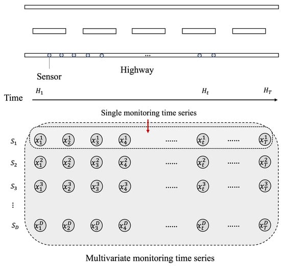
Figure 1.
Schematic illustration of the process for converting traffic flow data into a multivariate time series. With D sensors recording data over T time points, aligning the measurements by timestamp produces a set of multivariate sequences. Formally, if denotes the monitoring sequence of the d-th sensor; the resulting multivariate time series can be expressed as .
In practice, unexpected factors such as sensor malfunctions frequently lead to incomplete traffic flow datasets, resulting in the loss of certain observations. Such missing intervals are often continuous in nature (e.g., as illustrated by the blue-highlighted region in Figure 2, which shows three consecutive missing time steps). To allow the model to process sequences containing missing entries, we assign whenever the measurement is unavailable. However, this strategy risks conflating absent values with genuine zero readings. To address this, we introduce a masking vector to explicitly indicate the presence or absence of each measurement in . Denoting the d-th element of as , the vector is defined as
Write as a mask matrix.
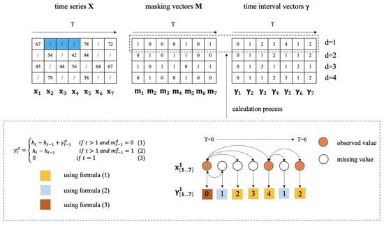
Figure 2.
Example of a multivariate time series with four dimensions and a sequence length of seven, containing several missing entries. The two sequences on the right correspond to the masking vector and the time interval vector . The computation of is based on the observation times of to , which are given by . The lower panel illustrates the derivation of the interval vector for the second dimension.
We introduce to denote the elapsed time since the most recent valid observation for a given feature. This variable serves to capture historical patterns of data absence, which can provide valuable contextual information for the downstream model. Let denote the timestamp at step t and the missing indicator of the d-th sensor at time t. The value of can then be formulated as
where is used to represent the d-th element in . Write as the attenuation matrix.
Consider the case where, at timestamp t, the reading from sensor d is unavailable, i.e., is unobserved. The goal is to estimate as an approximation to the true value. In most existing approaches for traffic flow data imputation, is inferred using other measurements from the same sensor , where . Such strategies rely solely on the temporal continuity of the individual monitoring sequence, neglecting spatial information from other sensors. Conversely, some methods draw upon readings from different sensors () at the same timestamp, yet they disregard temporal dependencies from other time steps. As noted earlier, traffic flow data exhibit pronounced spatio-temporal dependencies—both within a single stream (intra-flow) and across different streams (cross-flow). Existing interpolation techniques struggle to simultaneously account for both aspects. To address this limitation, we propose TSFNN, a framework that generates an estimate by jointly leveraging intra-stream and inter-stream correlations, thereby capturing both temporal and spatial dependencies in a unified manner.
The aim of the TSFNN framework is to define a mapping function capable of accurately interpolating missing entries such that the predicted values are consistent with the underlying distribution of the original dataset. This objective can be formulated as minimizing the interpolation error. In this work, the absolute error is adopted as the loss metric. Let denote the ground-truth value for sensor d at time t, which is unobserved in the dataset, and let represent the corresponding estimate derived from the available observations. The absolute loss is then expressed as . The interpolation task can thus be reframed as finding a function that satisfies
where represents the averaging operator.
3.2. Framework of TSFNN
As shown in Figure 3, the TSFNN framework is composed of two main interpolation components: the Temporal Module and the Spatial Module. The temporal module aims to extract temporal patterns from the data streams of individual sensors, thereby modeling their dynamics over time. In contrast, the spatial module is responsible for capturing inter-sensor dependencies—especially among sensors operating in similar environments—and for refining the predictions produced by the temporal module. The detailed architecture of the proposed framework is presented in Figure 4.
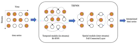
Figure 3.
Framework of TSFNN. White circles denote missing values, black lines indicate the connections between observed and missing values within each layer, and blue lines depict the links between interpolation results.
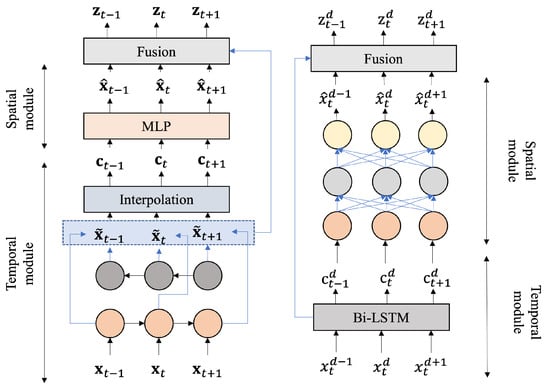
Figure 4.
Architecture of TSFNN. The diagram on the left depicts the component responsible for capturing temporal features, while the diagram on the right illustrates the component dedicated to capturing spatial features.
In the proposed framework, the temporal module is implemented using a Recurrent Neural Network (RNN)-based architecture, while the spatial module is constructed with an enhanced Multilayer Perceptron (MLP). Next, we introduce the temporal module in detail in Section 3.2.1, spatial module in Section 3.2.2, the combination method in Section 3.2.3, and the error/loss in Section 3.2.4.
3.2.1. Temporal Module
The temporal module is implemented through a function operating within each data stream. In our framework, is realized using a Long Short-Term Memory (LSTM) network. The structure of LSTM is shown in Figure 5.
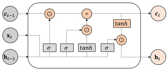
Figure 5.
Architecture of LSTM unit. In the figure, represents hidden state, indicates data, stands for cell state, means sigmoid function, stands for tanh function, and ⊙ represents the element-wise multiplication.
The LSTM [26] is designed to model sequential data and capture long-range temporal dependencies. By incorporating gating mechanisms, it mitigates the vanishing gradient problem commonly observed in conventional RNNs. An LSTM unit contains a memory cell, denoted as , along with three gates: the input gate , the forget gate , and the output gate . The memory cell retains or discards information depending on the signals from these gates, while the gates regulate the flow of information through the sequence. This process can be described as
where represents the sigmoid function, stands for the tanh function, and ⊙ indicates the element-wise multiplication. The trainable parameters of the model include the weight matrices and , as well as the bias vector .
To comprehensively capture temporal dependencies in the data, a bidirectional LSTM (Bi-LSTM) [27] is employed in constructing the temporal module. In this configuration, the forward hidden state at time t receives input from step , while the backward hidden state receives input from step . This design ensures that is not directly used when estimating . The mathematical formulation of the Bi-LSTM model is given as follows:
Here, the arrows indicate the forward and backward directions of information flow. The operator ⊙ denotes element-wise multiplication, while ∘ represents the concatenation operation. The variables and correspond to the hidden states from the preceding time step in the forward and backward passes, respectively. The parameters , , and represent the trainable weight matrices and bias vectors.
Equation (9) functions as the regression component, mapping the forward hidden state and the backward hidden state to the predicted vector . In Equations (10) and (12), two temporal decay factors, and , are applied to attenuate and , respectively. Conceptually, as or increases—signifying a longer interval since the last observation—the associated decay factor or decreases, thereby intensifying the attenuation of the hidden states. In other words, as the current time step becomes more distant from the nearest observed value, the impact of or on estimating diminishes. These decay factors represent the temporal missing patterns inherent in the sequence, which are essential for achieving accurate interpolation [14]. Equations (11) and (13) update the forward and backward hidden states, respectively, using the corresponding decayed hidden state from the prior step. At this stage, only intra-stream temporal relationships are captured, and the resulting estimates serve as intermediate outputs rather than the final interpolation results.
3.2.2. Spatial Module
The spatial module aims to model inter-flow dependencies, interpreted as spatial correlations between sensors. In real-world scenarios, sensors situated in similar environments frequently display analogous data patterns, which can appear as either positive or negative correlations. Therefore, estimation can be influenced by ( represents the monitoring data which have been preliminarily imputed by ). Moreover, the strength of the mutual dependency between two sensors is generally inversely related to the physical distance separating them. In practice, spatial relationships are implicitly encoded within the multiple data streams originating from monitoring datasets. Such latent structures can be identified and learned through appropriate computational techniques.
The spatial module implements a cross-stream interpolation function U. We define
where denotes the data vector at timestamp , which includes the in-stream estimates obtained at this step. This formulation ensures that the estimation leverages information from other data streams at the same time step, thereby eliminating the direct influence of its own prior estimation. The function U is realized using a Multilayer Perceptron (MLP). Let represent the spatial estimation vector, whose mathematical expression is given by
where and are parameters, and perform as sigmoid functions. The diagonal value of the parameter matrix is set to 0 to ensure that the estimated value is not affected by . Note that in this design, we do not explicitly use a spatial distance matrix or sensor adjacency graph. Instead, spatial relationships are implicitly learned through the MLP layer, which captures co-occurrence patterns across sensors. The diagonal masking of ensures that the imputation for each sensor is influenced only by other sensors, allowing the model to learn asymmetric but structured dependencies directly from data.
3.2.3. Spatial–Temporal Fusion Module
Figure 4 illustrates the full architecture of the TSFNN model. The two intermediate estimates generated within the framework have distinct emphases: the left one focuses on temporal dependencies within each individual flow, whereas the right one models spatial correlations among different flows. To merge these complementary outputs, we employ a weighting factor that fuses the temporal estimate with the spatial estimate , guided by the temporal gap indicators and . Let represent the final result of the interpolation process, which is expressed as
Here, the weight vector satisfies . In Equation (16), the spatial estimate is derived from , where each element of may correspond either to an actual observation or to a temporally interpolated value. To adaptively learn the weighting coefficients, we incorporate the time interval vectors and together with the masking vector , as formulated in Equation (17).
3.2.4. Loss Function
Our goal is to reduce estimation errors while preserving a distribution of interpolated data that aligns closely with that of the original dataset. Since all missing entries are masked during training, the true distribution of unobserved values is inaccessible. To address this, we promote distributional consistency by matching the estimated values within observed segments to the corresponding actual data points, thereby approximating the overall distribution of the complete dataset. Thus, we use the observed values to calculate the error, that is, the error between the estimated and the observed values. The absolute error is used as the loss for the estimate above, and the mean absolute error (MAE) is employed as the total loss for the entire dataset. This loss can be defined as
The model is updated by minimizing the loss .
3.3. Evaluation Metrics
Interpolation accuracy was assessed using the mean absolute error (MAE) and root mean square error (RMSE), two standard metrics for regression tasks. Regression models estimate mathematical relationships by analyzing associations between features and targets. The MAE reflects the average absolute deviation between predictions and ground truth in the same units as the data, making it straightforward to interpret. The RMSE has a similar formulation but penalizes larger deviations more heavily due to the squaring operation.
Let be the estimated value for a missing entry in dimension d at time t, the corresponding ground truth, and the mask indicating whether the entry is included in evaluation. The MAE and RMSE are computed as
4. Experiment
4.1. Datasets
We evaluated our model’s performance on four widely used real-world traffic datasets, PeMS03, PeMS04, PeMS07, and PeMS08, all sourced from the Caltrans Performance Measurement System (https://pems.dot.ca.gov/ (accessed on 12 February 2024)). Each dataset records the volume of vehicles passing through each sensor at 5-min intervals, resulting in 288 time steps per day per sensor.
4.1.1. Dataset Missing Value Manufacturing
To assess TSFNN’s ability to interpolate multivariate time series under various defect rates, we introduced controlled missingness into the dataset. Specifically, continuous temporal gaps were created to mimic consecutive missing segments, while additional values were removed following a Missing Completely at Random (MCAR) scheme. This process produced a hybrid missing pattern that combines sequential and random deletions, enabling a thorough evaluation of the model’s performance.
4.1.2. Data Normalization
To ensure fair comparison and minimize the influence of scale differences among features, a standard normalization step was applied in preprocessing. In particular, zero-mean normalization [28] was used, with each feature standardized based on its mean and variance computed from the original dataset.
4.2. Experimental Settings
4.2.1. Reproducibility
The dimension of the hidden state was fixed to 64. The temporal module, spatial module, and the LSTM and MLP layers contained within them all only had a single layer. We adopted ReLU as the activation function in the MLP components and tanh/sigmoid (inherent to LSTM) for the temporal module. The model was trained using the Adam optimizer with an initial learning rate of , which was adaptively adjusted during training. A learning rate scheduler with a patience of 10 epochs and a decay factor of was employed. The training used a batch size of 64 for up to 1000 epochs, with the sampling window size n fixed at 10.
Our model contains a total of 313,401 trainable parameters, corresponding to a memory size of approximately 1.20 MB under 32-bit floating point precision. On average, each training epoch took 7 s, and the full inference process required around 10 s on the CPU i7-12700H (Intel, Santa Clara, CA, USA), with a frequency of 2.30 GHz and GPU RTX 3090 (NVIDIA, Santa Clara, CA, USA).
4.2.2. Baselines
We selected ten widely used baselines to evaluate the performance of TSFNN. The traditional machine learning and statistical methods included the following:
- (1)
- Mean [1]: This method replaces missing values (with 0 for observations that are missing) by averaging the preceding and succeeding observations.
- (2)
- This approach identifies the k-nearest neighbors of a given sample and computes their mean value to perform interpolation. For the dataset used in this study, the best performance was obtained with .
- (3)
- MissRandomForest (MRF) [10]: This method is a widely adopted strategy for handling missing data, leveraging the random forest algorithm to predict and impute missing values iteratively.
The deep learning-based methods included the following:
- (1)
- RNN [14]: This method utilizes an LSTM-based architecture to model temporal dependencies, with the specific aim of imputing missing values.
- (2)
- Bi-RNN [27]: This method extends the RNN method to bidirectional and uses bidirectional LSTM for more complete learning of temporal information.
- (3)
- TIDER [22]: A deep learning model for multivariate time series imputation, which enhances the imputation effect by decoupling time dynamic factors such as trend, periodicity, and residual.
- (4)
- GRIN [23]: A bidirectional graph Recurrent Neural Network consisting of two unidirectional GRIN sub-modules that perform two-stage interpolation for each direction, thereby processing the input sequence progressively in both forward and backward directions over time.
- (5)
- TimesNet [24]: This model employs a modular architecture to decompose complex temporal dynamics into multiple cycles and achieves unified modeling of both intra-cycle and inter-cycle variations by transforming the original one-dimensional time series into a two-dimensional representation.
- (6)
- Transformer: Directly uses an attention mechanism for imputation.
- (7)
- DLinear [25]: Decomposes the original sequence into two parts, trend and seasonality, typically through simple methods such as moving averages. It models the trend and seasonal components separately using independent linear layers and then combines the output results to obtain the final prediction value.
4.3. Main Result
As shown in Table 1 and Table 2, the MEAN method consistently produce the lowest accuracy across all tested missing rates. This limitation arises from its simplistic strategy of interpolating by averaging the values immediately before and after the gap, which performs poorly when faced with long sequences of missing data or pronounced nonlinear patterns. In contrast, the two traditional machine learning approaches, KNN and MRF, achieved markedly better results. KNN identified the nearest neighbors of a missing point based on the Euclidean distance and imput its value using their mean, enabling more relevant reference points than the MEAN method, thus yielding higher accuracy. The MRF, on the other hand, estimated missing entries by iteratively building decision trees, focusing on modeling the dataset’s overall trend rather than depending solely on local information, which enhanced its interpolation effectiveness. The RNN adopted a unidirectional architecture to learn temporal information, which can better capture temporal features than previous methods and thus deduce the overall trend of the data. However, due to the temporal nature of the sequence, the information learned from one-way learning often could not cover the complete information of the data well, so there are certain limitations in its interpolation. Bi-RNN adopted a bidirectional RNN architecture to learn the temporal information of data from both positive and negative directions, striving to comprehensively capture temporal relationships. When the missing rate is relatively low, RNN-based methods may not be as effective as the previous machine learning algorithms. When the missing rate increases, the advantages of RNN methods become reflected. TIDER and DLinear relied on explicit decomposition of temporal components (e.g., trend and seasonality), which helped under regular patterns but limited their flexibility in complex traffic data. GRIN modeled bidirectional temporal and graph structures but was sensitive to high missing ratios due to accumulated errors. TimesNet captured periodicity effectively but lacked spatial modeling. Transformer performed moderately but suffered from disrupted attention when missing rates are high. TSFNN exhibited the best performance at different missing rates due to its combination of spatial features. We selected four datasets with 70% missing values to illustrate, as depicted in Figure 6. As shown in the figure, the filling curve of our method closely aligns with the true values, demonstrating the effectiveness of our model. The performance of these methods deteriorates as the missing rate increases. This is partly due to the remaining data becoming increasingly sparse and the need to extract fewer feature information.

Table 1.
Results of MAE (lower is better). The best result is indicated in bold.
Table 2.
Results of RMSE (lower is better). The best result is indicated in bold.
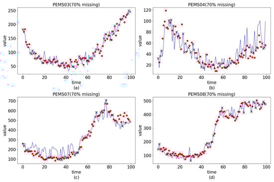
Figure 6.
The black crosses denote the observed values, the red circles indicate the ground-truth targets for imputation, and the blue curve illustrates the interpolation results.
4.4. Ablation Experiment
In contrast to standard RNN frameworks, TSFNN integrates a spatial interpolation module in addition to its temporal interpolation component. Furthermore, the temporal module adopts a bidirectional interpolation design, setting it apart from conventional RNN-based methods. To evaluate the role of each architectural element, we conducted ablation studies in which specific modules were removed or altered. The resulting model variants are outlined as follows:
- TSFNN-t: This variant removes the temporal module from TSFNN, thereby relying solely on the spatial module to capture spatial dependencies without modeling temporal correlations.
- TSFNN-s: This variant removes the spatial interpolation module from TSFNN, thereby relying solely on the temporal module to capture temporal dependencies without modeling spatial correlations.
- TSFNN-bi: This variant modifies the temporal module by replacing the bidirectional structure with a unidirectional structure, thereby capturing temporal dependencies in only one direction.
Table 3 and Table 4 demonstrate that TSFNN outperformed all the variant models, and its superiority became increasingly evident on all datasets as the missing rate increased. The results of TSFNN-t demonstrate that using MLP alone to extract spatial correlation information for input missing data is clearly not sufficient to achieve good interpolation results. This emphasizes the basic requirement of capturing temporal correlations to effectively estimate traffic data. These results highlight the crucial role of temporal correlation modeling in accurately estimating traffic data. Substituting the temporal module’s bidirectional structure with a unidirectional one, as in TSFNN-b, led to a noticeable drop in interpolation accuracy. This decline stems from the reduced capacity to learn contextual temporal dependencies in both directions, weakening data reconstruction and, consequently, interpolation quality. Similarly, removing the spatial module in TSFNN-s resulted in poorer outcomes, underscoring that spatial dependency modeling is equally vital for effective interpolation. Taken together, the findings indicate that every component within TSFNN plays a significant part in achieving its overall performance.
Table 3.
Ablation experimental results of MAE (lower is better). The best result is indicated in bold.
Table 4.
Ablation experimental results of RMSE (lower is better). The best result is indicated in bold.
5. Conclusions
In this work, we adopted the TSFNN to investigate traffic flow datasets affected by various missing ratios and sequences of continuous data loss. Unlike conventional methods that often neglect either temporal or spatial dependencies, the proposed framework simultaneously leverages both to guide the imputation process. By capturing these spatio-temporal patterns, the TSFNN reconstructs incomplete data more precisely, improving overall dataset integrity and supporting reliable stability assessments.
The main contributions are as follows:
- By utilizing time and space modules aimed at capturing temporal and spatial correlations, we effectively alleviate the traditional challenges outlined earlier. The temporal module integrates a bidirectional LSTM architecture, which helps to enhance the capture of temporal dependencies. Meanwhile, the spatial module utilizes MLP to proficiently capture spatial correlations.
- The experimental results show that the TSFNN achieves improvements in the RMSE compared to benchmark approaches, including MEAN, KNN, MRF, RNN, and Bi-RNN. This demonstrates the framework’s advantage in interpolation accuracy.
- From the ablation experiment, it can be seen that each module of the TSFNN has a unique role and is indispensable.
Although our experiments were conducted on freeway-based PeMS datasets, the modular design of TSFNN is not specific to highway scenarios. The separation of temporal and spatial modules allows it to adapt to other traffic environments, such as arterial roads and urban intersections, which also exhibit spatio-temporal patterns. Furthermore, the framework is potentially applicable to other domains involving spatio-temporal missing data, such as meteorological forecasting, environmental sensing, or healthcare monitoring. Future work will explore domain adaptation to broaden the TSFNN’s applicability.
Author Contributions
Methodology, G.W.; Formal analysis, X.L.; Investigation, H.L.; Writing—original draft, Y.M.; Writing—review & editing, K.L. All authors have read and agreed to the published version of the manuscript.
Funding
This study received funding from the National Key R&D Program of China under grant 2022YFB2602103; the National Natural Science Foundation of China under Grant No. U2469205; the Fundamental Research Funds for the Central Universities of China under Grant No. JKF-20240769; the Beijing Nova Program under Grant No. 20230484353. The funder was not involved in the study design, collection, analysis, interpretation of data, the writing of this article, or the decision to submit it for publication.
Data Availability Statement
The original contributions presented in this study are included in the article. Further inquiries can be directed to the corresponding author.
Conflicts of Interest
All authors are affiliated with universities or public research institutions and have no commercial affiliations. The authors declare that the research was conducted in the absence of any commercial or financial relationships that could be construed as a potential conflicts of interest.
References
- Kreindler, D.M.; Lumsden, C.J. The Effects of the Irregular Sample and Missing Data in Time Series Analysis. Nonlinear Dyn. Psychol. Life Sci. 2006, 10, 187–214. [Google Scholar]
- Benesty, J.; Chen, J.; Huang, Y. Time-delay estimation via linear interpolation and cross correlation. IEEE Trans. Speech Audio Process. 2004, 12, 509–519. [Google Scholar] [CrossRef]
- Gasca, M.; Sauer, T. Polynomial interpolation in several variables. Adv. Comput. Math. 2000, 12, 377–410. [Google Scholar] [CrossRef]
- McKinley, S.; Levine, M. Cubic spline interpolation. Coll. Redwoods 1998, 45, 1049–1060. [Google Scholar]
- Luo, X.; Meng, X.; Gan, W.; Chen, Y. Traffic data imputation algorithm based on improved low-rank matrix decomposition. J. Sens. 2019, 2019, 7092713. [Google Scholar] [CrossRef]
- Mazumder, R.; Hastie, T.; Tibshirani, R. Spectral regularization algorithms for learning large incomplete matrices. J. Mach. Learn. Res. 2010, 11, 2287–2322. [Google Scholar]
- Yu, H.-F.; Rao, N.; Dhillon, I.S. Temporal regularized matrix factorization for high-dimensional time series prediction. Adv. Neural Inf. Process. Syst. 2016, 29, 847–855. [Google Scholar]
- Schnabel, T.; Swaminathan, A.; Singh, A.; Chandak, N.; Joachims, T. Recommendations as treatments: Debiasing learning and evaluation. In Proceedings of the 33rd International Conference on Machine Learning, New York, NY, USA, 20–22 June 2016. [Google Scholar]
- Al-Douri, Y.K.; Hamodi, H.; Lundberg, J. Time series forecasting using a two-level multi-objective genetic algorithm: A case study of maintenance cost data for tunnel fans. Algorithms 2018, 11, 123. [Google Scholar] [CrossRef]
- Stekhoven, D.J.; Bühlmann, P. MissForest—Non-parametric missing value imputation for mixed-type data. Bioinformatics 2012, 28, 112–118. [Google Scholar] [CrossRef]
- Qian, C.; Chen, J.; Luo, Y.; Dai, L. Random forest based operational missing data imputation for highway tunnel. J. Transp. Syst. Eng. Inf. Technol. 2016, 16, 81. [Google Scholar]
- Zhang, J.; Li, D.; Wang, Y. Predicting tunnel squeezing using a hybrid classifier ensemble with incomplete data. Bull. Eng. Geol. Environ. 2020, 79, 3245–3256. [Google Scholar] [CrossRef]
- Kim, B.; Lee, D.-E.; Preethaa, K.R.S.; Hu, G.; Natarajan, Y.; Kwok, K.C.S. Predicting wind flow around buildings using deep learning. J. Wind. Eng. Ind. Aerodyn. 2021, 219, 104820. [Google Scholar] [CrossRef]
- Che, Z.; Purushotham, S.; Cho, K.; Sontag, D.; Liu, Y. Recurrent neural networks for multivariate time series with missing values. Sci. Rep. 2018, 8, 6085. [Google Scholar] [CrossRef]
- Guo, D.; Li, J.; Li, X.; Li, Z.; Li, P.; Chen, Z. Advance prediction of collapse for TBM tunneling using deep learning method. Eng. Geol. 2022, 299, 106556. [Google Scholar] [CrossRef]
- Adeyemi, O.; Grove, I.; Peets, S.; Domun, Y.; Norton, T. Dynamic neural network modelling of soil moisture content for predictive irrigation scheduling. Sensors 2018, 18, 3408. [Google Scholar] [CrossRef]
- Liang, Y.; Jiang, K.; Gao, S.; Yin, Y. Prediction of tunnelling parameters for underwater shield tunnels, based on the GA-BPNN method. Sustainability 2022, 14, 13420. [Google Scholar] [CrossRef]
- Wang, Y.; Pang, Y.; Song, X.; Sun, W. Tunneling Operational Data Imputation with Radial Basis Function Neural Network. In Proceedings of the International Joint Conference on Energy, Electrical and Power Engineering, Melbourne, VIC, Australia, 22–24 November 2023. [Google Scholar]
- González-Vidal, A.; Rathore, P.; Rao, A.S.; Mendoza-Bernal, J.; Palaniswami, M.; Skarmeta-Gómez, A.F. Missing data imputation with bayesian maximum entropy for internet of things applications. IEEE Internet Things J. 2020, 8, 16108–16120. [Google Scholar] [CrossRef]
- Wang, G.; Deng, Z.; Choi, K.S. Tackling missing data in community health studies using additive LS-SVM classifier. IEEE J. Biomed. Health Inform. 2016, 22, 579–587. [Google Scholar] [CrossRef]
- Erhan, L.; Di Mauro, M.; Anjum, A.; Bagdasar, O.; Song, W.; Liotta, A. Embedded data imputation for environmental intelligent sensing: A case study. Sensors 2021, 21, 7774. [Google Scholar] [CrossRef]
- Liu, S.; Li, X.; Cong, G.; Chen, Y.; Jiang, Y. Multivariate time-series imputation with disentangled temporal representations. In Proceedings of the Eleventh International Conference on Learning Representations, Kigali, Rwanda, 1–5 May 2023. [Google Scholar]
- Cini, A.; Marisca, I.; Alippi, C. Filling the g_ap_s: Multivariate time series imputation by graph neural networks. arXiv 2021, arXiv:2108.00298. [Google Scholar]
- Wu, H.; Hu, T.; Liu, Y.; Zhou, H.; Wang, J.; Long, M. Timesnet: Temporal 2d-variation modeling for general time series analysis. arXiv 2022, arXiv:2210.02186. [Google Scholar]
- Zeng, A.; Chen, M.; Zhang, L.; Xu, Q. Are transformers effective for time series forecasting? Proc. AAAI Conf. Artif. Intell. 2023, 37, 11121–11128. [Google Scholar] [CrossRef]
- Graves, A.; Graves, A. Long short-term memory. In Supervised Sequence Labelling with Recurrent Neural Networks; Springer: Berlin/Heidelberg, Germany, 2012; pp. 37–45. [Google Scholar] [CrossRef]
- Zhou, P.; Shi, W.; Tian, J.; Qi, Z.; Li, B.; Hao, H.; Xu, B. Attention-Based Bidirectional Long Short-Term Memory Networks for Relation Classification. In Proceedings of the 54th Annual Meeting of the Association for Computational Linguistics, Berlin, Germany, 7–12 August 2016; Volume 2. Short papers. [Google Scholar]
- Meulman, J.J. Optimal Scaling Methods for Multivariate Categorical Data Analysis. SPSS White Paper Chicago 1998. Available online: https://www.researchgate.net/profile/Jacqueline-Meulman/publication/268274402_Optimal_scaling_methods_for_multivariate_categorical_data_analysis/links/553625040cf218056e92cab7/Optimal-scaling-methods-for-multivariate-categorical-data-analysis.pdf (accessed on 5 April 2024).
Disclaimer/Publisher’s Note: The statements, opinions and data contained in all publications are solely those of the individual author(s) and contributor(s) and not of MDPI and/or the editor(s). MDPI and/or the editor(s) disclaim responsibility for any injury to people or property resulting from any ideas, methods, instructions or products referred to in the content. |
© 2025 by the authors. Licensee MDPI, Basel, Switzerland. This article is an open access article distributed under the terms and conditions of the Creative Commons Attribution (CC BY) license (https://creativecommons.org/licenses/by/4.0/).