Orthogonal-Constrained Graph Non-Negative Matrix Factorization for Clustering

Abstract

We propose a novel approach for clustering problem, which refers to as Graph Regularized Orthogonal Subspace Non Negative Matrix Factorization (GNMFOS). This type of model introduces both graph regularization and orthogonality as penalty terms into the objective function. It not only obtains the uniqueness of matrix decomposition but also improves the sparsity of decomposition and reduces computational complexity. Most importantly, using the idea of iteration under weak orthogonality, we construct an auxiliary function for the algorithm and obtain convergence proof to compensate for the lack of convergence proof in similar models. The experimental results show that compared with classical models such as GNMF and NMFOS, our algorithm significantly improves clustering performance and the quality of reconstructed images.

1. Introduction

Clustering is a fundamental technique in data analysis, extensively applied in image processing, document classification, and other fields. As an unsupervised learning method, it aims to partition a dataset into distinct groups such that data points within the same group are more similar to each other than to those in different groups. Common clustering algorithms determine the relationship between data points by measuring their similarity, and assign data points with similar features to the same cluster. Due to the non-negativity requirement in many real-world applications, Non-negative Matrix Factorization (NMF) has attracted considerable attention as a dimensionality reduction and clustering technique. NMF effectively reduces storage cost and computation complexity by producing interpretable parts-based representations. NMF has been successfully applied and extended to various domains including clustering and classification [1,2,3], image analysis [4,5,6], spectral analysis [7,8], and blind source separation [9,10]. More recently, NMF-related methods have also found applications in micro-video classification [11], RNA-seq data deconvolution [12], attributed network anomaly detection [13], and signal processing tasks such as dynamic spectrum cartography and tensor completion [14], which further demonstrate the method’s adaptability and growing relevance.

Various extensions of NMF have been proposed to capture the latent structures within data. For example, Cai et al. [15] proposed Graph Regularized NMF (GNMF) by incorporating a graph Laplacian term into the objective function, enabling the preservation of intrinsic geometric structure. Hu et al. [16] further introduced GCNMF by integrating GNMF with Convex NMF. Meng et al. [17] extended the regularization to both the sample and feature spaces, resulting in the Dual-graph Sparse NMF (DSNMF) method. Other notable variants include GDNMF [18], DNMF [19], RHDNMF [20], AWMDNMF [21], TGLMC [22], and PGCNMF [23], each offering improvements for non-linear or structured data modeling.

In the context of image clustering, Li et al. [24] observed that local representations are often associated with orthogonality. Ding et al. [25] introduced Orthogonal NMF (ONMF), demonstrating that orthogonality enhances sparsity, reduces redundancy, and improves the interpretability and uniqueness of clustering results. However, enforcing strict orthogonality often leads to high computational cost, especially for large document datasets.

To overcome such problems, researchers have proposed a series of methods with orthogonal constraints [26,27,28]. Unfortunately, among the existing results (to the best of our ability to search for all existing results), there is a lack of NMF methods that simultaneously consider the orthogonality of coefficient matrices in orthogonal subspaces and the intrinsic geometric structures hidden in data and feature manifolds. Or, even if a similar model is proposed, the convergence proof of the update algorithm is missing or incorrect.

In this paper, we propose a novel approach that combines graph Laplacian and nonnegative matrix factorization in orthogonal subspaces. The generation of orthogonal factor matrices is incorporated as a penalty term into the objective function, along with the addition of a graph regularization term. On one hand, by introducing orthogonal penalties and graph Laplacian terms, the orthogonality of the factor matrices is achieved through the factorization process, reducing the computational burden imposed by enforcing orthogonality constraints. On the other hand, it enhances sparsity in the coefficient matrix to some extent and utilizes the geometric structure properties of the data, thereby improving the ability to recover underlying nonlinear relationships. We have uniformly named this series of models as Graph Regularized Nonnegative Matrix Factorization on Orthogonal Subspace (GNMFOS), and of course, some special cases will be annotated with lowercase letters and numbers, such as GNMFOSv2. We develop two efficient algorithms to solve the proposed models and demonstrate their convergence. Moreover, we construct the objective function of GNMFOS using Euclidean distance and optimize it using the MUR. Finally, we conduct experiments to evaluate the proposed algorithms. The experimental results show that GNMFOS and GNMFOSv2 combine the advantages of previous algorithms, resulting in improved effectiveness and robustness.

In this study, the orthogonal constraints in matrix factorization inherently exhibit mathematical symmetry, ensuring balanced and reciprocal relationships between data representations. This symmetry not only simplifies the computational model but also enhances the interpretability of clustering results.

The remaining contents of this paper are as follows. Section 2 presents a review of related work, including NMF, NMFOS, and GNMF. Section 3 provides a detailed description of our proposed method, including the derivation of update rules and corresponding algorithms. Section 3 also presents the convergence analysis of the algorithms. Section 4 will show experimental results and the relevant analysis. Section 5 is a summary of the paper and also discusses future research directions.

2. Preliminaries

In this section, we will introduce some symbols in Table 1, then introduce some models and related works to serve as the foundation for our paper.

Table 1. Important symbols annotated in this paper.

Symbols	Description
$\mathbb{N}$	The set of all natural numbers
$R_{+}^{\upsilon \times \omega }$	The set of all nonnegative matrices with $\upsilon ,\omega \in \mathbb{N}$
X	Input nonnegative data matrix $X=[x_1,\dots ,x_N]\in R_{+}^{M\times N}$
W	The basis matrix $W=\left[w_{ik}\right]\in R_{+}^{M\times K}$
H	The coefficient matrix $H=\left[h_{kj}\right]\in R_{+}^{K\times N}$
M	The number of data features(or denoted as data dimension)
N	The number of data instances(or denoted as data points)
K	The number of data clusters
i	Elements in the sets $\{1,2,\dots ,M\}$
j	Elements in the sets $\{1,2,\dots ,N\}$
k	Elements in the sets $\{1,2,\dots ,K\}$
${\parallel ·\parallel }_F$	Frobenius norm
$Tr(·)$	The trace operator
L	The graph Laplacian operators of the data manifold
S	The weighted matrix
D	The diagonal matrices with $D_{ii}={\sum }_j{S}_{ij}$
p	The size of nearestneighbors
I	The identity matrix
$\alpha$	The penalty parameter for controlling orthogonality $\alpha \ge 0$
$\lambda$	The regularization parameter $\lambda \ge 0$
$\psi ,\varphi$	Lagrange multiplier

2.1. NMF

The classical NMF [29] is a nonnegative matrix factorization algorithm that focuses on analyzing data matrices consisting of nonnegative elements. Given a nonnegative data matrix X, the aim of NMF is to find two nonnegative matrices W and H, such that the product of W and H can closely approximate the original matrix X, i.e.,

The optimization model for NMF can be formulated as follows:

$$\begin{array}{c}\underset{W,H}{min}{\parallel X-WH\parallel }_F^2,\hfill \\ s.t.W\ge 0,H\ge 0.\hfill \end{array}$$

2.2. NMFOS

Although NMF has many advantages, it is not easy to obtain the desired solution. Chris Ding et al. [25] extended the traditional NMF by adding an orthogonal constraint on the basis or coefficient matrix into the objective function’s constraints. Li et al. [30] optimized the above model; they proposed a novel approach called Nonnegative Matrix Factorization with Orthogonal Subspace (NMFOS), which is based on the idea of putting the orthogonality as a penalty term into the objective function, and obtained the following new model.

$$\begin{array}{cc}\hfill & \underset{W,H}{min}{\parallel X-WH\parallel }_F^2+\alpha {\parallel H{H}^T-I\parallel }_F^2,\hfill \\ & s.t.W\ge 0,H\ge 0.\hfill \end{array}$$

Here, the orthogonality of H is shown (and G’s is $G^{T}G$) with parameter $\alpha \ge 0$ controlling the orthogonality of the vectors in H.

2.3. GNMF

Graph regularization is a data processing method based on manifolds. The core concept is that manifolds can enhance the smoothness of data in linear and nonlinear spaces by minimizing (1) beolw. As demonstrated by existing studies, incorporating the geometric structure information from data points can enhance the clustering performance of NMF [31,32]. So, the p-nearest neighbor graph is constructed based on the input data matrix X to effectively capture the geometric structure. Meanwhile, in order to characterize the similarity between adjacent points, a weight matrix $S=\left\{S_{jl}\right\}$ is defined. In this paper, the $0-1$ weight matrix below is commonly used.

$$\begin{array}{c}\hfill S_{jl}=\left\{\begin{array}{cc}1,\hfill & x_j\in N\left(x_l\right)\mathrm{or}{x}_l\in N\left(x_j\right),\hfill \\ 0,\hfill & \mathrm{otherwise},\hfill \end{array}\right.j,l\in \{1,\dots ,N\}.\end{array}$$

Here, $N\left(x_j\right)$ represents the set of p-nearest neighbors for data point $x_j$. There are many options for defining $S=\left\{S_{jl}\right\}$ containing heat kernal weight matrix $S_{jl}=e^{-{\displaystyle \frac{\parallel {\mathbf{x}}_j-{\mathbf{x}}_l{\parallel }^2}{\sigma }}}$ and dot-product weight matrix $S_{jl}=x_j^T{x}_l.$ With the help of the weight matrix S, the Laplacian matrix L is defined to characterize the degree of similarity between points in geometric structure and $L=D-S$, where D is the degree matrix with $D_{ii}={\sum }_j{S}_{ij}$. Inspired by manifold learning, Cai et al. [15] proposed the GNMF algorithm. The core idea is the graph regularization

$$\begin{array}{cc}\hfill & {\displaystyle \frac{1}{2}}\sum _{l=1}^n\sum _{j=1}^n{\parallel h_l-h_j\parallel }_2^2{S}_{lj}=\sum _{j=1}^n{D}_{jj}{h}_j^T{h}_j-\sum _{l=1}^n\sum _{j=1}^n{S}_{lj}{h}_l^T{h}_j\hfill \\ \hfill & =Tr\left(HD{H}^T\right)-Tr\left(HS{H}^T\right)=Tr\left(HL{H}^T\right),\hfill \end{array}$$

(1)

Then, the optimization model of GNMF is given by

$$\begin{array}{cc}\hfill & min{∥X-WH∥}_F^2+\lambda Tr\left(HL{H}^T\right),\hfill \\ & s.t.W\ge 0,H\ge 0.\hfill \end{array}$$

In fact, the minimization of (1) shows that if two data points are close in original data’ distribution, they will also be close under the new basis vectors $h_l$ and $h_j$. The regularization parameter $\lambda \ge 0$ controls the smoothness of the model.

3. A New Model

In this section, we will combine NMFOS and GNMF to introduce a new method called Graph Regularized Non-negative Matrix Factorization on Orthogonal Subspaces (GNMFOS). More importantly, we also provide a convergence proof for this new model to compensate for the lack or inadequacy of algorithm convergence proof. Note that in order to enhance the clustering performance, our model GNMFOS integrates the advantages of existing methods.

3.1. GNMFOS

By putting both the orthogonality and the Graph Laplacian into the objective function, GNMFOS is formulated as follows.

$$\begin{array}{cc}\hfill & minJ(W,H)=\underset{W,H}{min}{\displaystyle \frac{1}{2}}{\parallel X-WH\parallel }_F^2+{\displaystyle \frac{\alpha }{4}}{\parallel H{H}^T-I\parallel }_F^2+{\displaystyle \frac{\lambda }{2}}Tr\left(HL{H}^T\right),\hfill \\ \hfill & s.t.W\ge 0,H\ge 0.\hfill \end{array}$$

(2)

where $X\in R_{+}^{M\times N}$, $W\in R_{+}^{M\times K}$, $H\in R_{+}^{K\times N}$. Considering the Lagrange function in (2), we obtain the following update rules.

$$\begin{array}{c}\hfill W_{ik}⟵W_{ik}{\displaystyle \frac{{\left(X{H}^T\right)}_{ik}}{{\left(WH{H}^T\right)}_{ik}}},\end{array}$$

(3)

$$\begin{array}{c}\hfill H_{kj}⟵H_{kj}{\displaystyle \frac{{\left(W^{T}X+\alpha H+\lambda HS\right)}_{kj}}{{\left(W^{T}WH+\alpha H{H}^{T}H+\lambda HD\right)}_{kj}}}.\end{array}$$

(4)

The update rule (3) and its convergence proof are the same as in [15]. But (4) is new and it is hard to prove its convergence directly, as the orthogonality of H requires handling the fourth power term of H, which makes it difficult to implement the commonly used approach of using second-order Taylor formula to construct auxiliary functions and further obtain convergence proofs for updating rules. To clarify this difficult task, the first and second derivatives of the objective function $J(W,H)$ with respect to $H_{kj}$ are given below.

$$\begin{array}{cc}\hfill F_{H_{kj}}^{\prime }& ={\left({\displaystyle \frac{\partial J(W,H)}{\partial H}}\right)}_{kj}={(W^{T}WH-W^{T}X+\alpha H{H}^{T}H-\alpha H+\lambda HL)}_{kj},\hfill \end{array}$$

$$\begin{array}{c}\hfill F_{H_{kj}}^{″}={(W^{T}W+\alpha H{H}^T-\alpha I)}_{kk}+{(\alpha H^{T}H+\lambda L)}_{jj}+\alpha H_{kj}^2.\end{array}$$

According to tradition, the auxiliary function of H should be defined as follows:

$$\begin{array}{cc}\hfill G_H(H_{kj},H_{kj}^t)& =F_{H_{kj}}\left(H_{kj}^t\right)+F_{H_{kj}}^{\prime }\left(H_{kj}^t\right)(H_{kj}-H_{kj}^t)\hfill \\ & +{\displaystyle \frac{1}{2}}{\displaystyle \frac{{(W^{T}W{H}^t+\alpha H^t{H^t}^T{H}^t+\lambda H^{t}D)}_{kj}}{H_{kj}^t}}{(H_{kj}-H_{kj}^t)}^2.\hfill \end{array}$$

So, we can ensure that ${\displaystyle \frac{\partial G_H(H_{kj},H_{kj}^t)}{\partial H_{kj}}}=0$ leads to the same update rule in (4). Returning to the Taylor series expansion of $F_{H_{kj}}\left(H_{kj}\right)$, it is easy to obtain

$$\begin{array}{cc}\hfill F_{H_{kj}}\left(H_{kj}\right)& =F_{H_{kj}}\left(H_{kj}^t\right)+F_{H_{kj}}^{\prime }\left(H_{kj}^t\right)(H_{kj}-H_{kj}^t)\hfill \\ & +{\displaystyle \frac{1}{2}}[{(W^{T}W+\alpha H^t{H^t}^T-\alpha I)}_{kk}+{(\alpha {H^t}^T{H}^t+\lambda L)}_{nn}]{(H_{kj}-H_{kj}^t)}^2.\hfill \end{array}$$

In this way, a difficulty of convergence proof between $G_H(H_{kj},H_{kj}^t)$ and $F_{H_{kj}}\left(H_{kj}\right)$ arises, i.e., when proving that the function $G_H(H_{kj},H_{kj}^t)$ is an auxiliary function, we cannot prove that

$${\displaystyle \frac{{\left(H^t{H^t}^T{H}^t\right)}_{kj}}{H_{kj}^t}}\ge {(H^t{H^t}^T-I)}_{kk}+{\left({H^t}^T{H}^t\right)}_{jj}+H_{kj}^2.$$

So, we improve (2) by proposing a new variant model where H is weakly orthogonal. This new model is called weakly orthogonal because it is obtained by orthogonalizing the t-th iteration of H with the (t − 1)-th iteration, where the t-th iteration is treated as an unknown variable and the (t − 1)-th iteration is treated as a constant ($t=1,2,\dots$). Then, the following new model is now arrived at.

$$\begin{array}{cc}\hfill & minJ(W,H^t,H^{t-1})=\underset{W,H}{min}{\displaystyle \frac{1}{2}}\parallel X-W{H}^t{\parallel }_F^2+{\displaystyle \frac{\alpha }{2}}{\parallel H^t{H}^{{t-1}^T}-I\parallel }_F^2+{\displaystyle \frac{\lambda }{2}}Tr\left(H^{t}L{H}^{t^T}\right),\hfill \\ \hfill & s.t.W\ge 0,H\ge 0.\hfill \end{array}$$

(5)

Here, $\alpha \ge 0$ and $\lambda \ge 0$ represent the orthogonal penalty parameter and regularization parameter, respectively. The parameter $\alpha$ is used to adjust the degree of orthogonality in H, while the parameter $\lambda$ balances the reconstruction error in the first term and the graph regularization in the third term of the objective function. It is worth mentioning that if the update rule for H converges, we have reason to suspect that $H^{t-1}$ approximates $H^t$, and $H^t{H}^{t-1^T}\approx H^t{H}^{t^T}$.

Due to the non-convexity of the objective function in both variables W and H in (5), we adopt an iterative optimization algorithm and utilize multiplicative update rules to obtain local optima (original idea comes from [33,34,35]). The variables W and H are updated alternately while keeping the other variable fixed.

We can rewrite the objective function of $J(W,H^t,H^{t-1})$ in trace form as follows.

$$\begin{array}{cc}\hfill J(W,H^t,H^{t-1})=& {\displaystyle \frac{1}{2}}Tr(X^{T}X-2X^{T}W{H}^t+H^{t^T}{W}^{T}W{H}^t)\hfill \\ & +{\displaystyle \frac{\alpha }{2}}Tr(H^{t-1}{H}^{t^T}{H}^t{H^{t-1}}^T-2H^{t-1}{H}^{t^T}+I)\hfill \\ & +{\displaystyle \frac{\lambda }{2}}Tr\left(H^{t}L{H}^{t^T}\right),\hfill \end{array}$$

where $\psi$ and $\varphi$ represent the Lagrange multipliers for $W\ge 0$ and $H\ge 0$ in (5), respectively. Let $\Psi =\left[{\psi }_{ik}\right],\Phi =\left[{\varphi }_{kj}\right]$, then, the Lagrangian function follows:

$$\begin{array}{cc}\hfill L& ={\displaystyle \frac{1}{2}}Tr(X^{T}X-2X^{T}W{H}^t+H^{t^T}{W}^{T}W{H}^t)\hfill \\ & +{\displaystyle \frac{\alpha }{2}}Tr(H^{t-1}{H}^{t^T}{H}^t{H^{t-1}}^T-2H^{t-1}{H}^{t^T}+I)\hfill \\ & +{\displaystyle \frac{\lambda }{2}}Tr\left(H^{t}L{H}^{t^T}\right)-Tr\left({\Psi }^T{H}^t\right)-Tr\left({\Phi }^{T}W\right).\hfill \end{array}$$

The function L solves for stable points of W and H, respectively, and obtains the following equations.

$$\begin{array}{c}\hfill \Psi =W{H}^t{H}^{t^T}-X{H}^{t^T},\end{array}$$

(6)

$$\begin{array}{c}\hfill \Phi =W^{T}W{H}^t-W^{T}X+\alpha H^t{H^{t-1}}^T{H}^{t-1}-\alpha H^{t-1}+\lambda H^{t}D-\lambda H^{t}S.\end{array}$$

(7)

With the help of KKT conditions ${\psi }_{ik}{W}_{ik}=0$ and ${\varphi }_{kj}{H}_{kj}^t=0$, multiplying both sides of (6) by $W_{ik}$ and (7) by $H_{kj}^t$, we will receive the iterative update rule for (5):

$$\begin{array}{c}\hfill W_{ik}^{t+1}⟵W_{ik}^t{\displaystyle \frac{{\left(X{H}^{t^T}\right)}_{ik}}{{\left(W^t{H}^t{H}^{t^T}\right)}_{ik}}},\end{array}$$

(8)

$$\begin{array}{c}\hfill H_{kj}^{t+1}⟵H_{kj}^t{\displaystyle \frac{{\left({W^{t+1}}^{T}X+\alpha H^{t-1}+\lambda H^{t}S\right)}_{kj}}{{\left({W^{t+1}}^T{W}^{t+1}{H}^t+\alpha H^t{H^{t-1}}^T{H}^{t-1}+\lambda H^{t}D\right)}_{kj}}}.\end{array}$$

(9)

In summary, we can now develop the efficient algorithm below to solve (5). For a detailed proof of the convergence of Algorithm 1, please refer to Appendix A.

Algorithm 1 GNMFOS

Input: Nonnegative data matrix $X=\left[x_1,\dots ,x_N\right]\in R_{+}^{M\times N}$, the number of clusters K, the orthogonality parameter $\alpha \ge 0$, the regularization parameter $\lambda \ge 0$, the maximum number of iterations T; Initialization randomly choose initial matrices $W^0\in R_{+}^{M\times K}$ and $H^0\in R_{+}^{K\times N}$ while The termination conditions are not satisfied or $t\le T$ do    Fixing H, updating W according to (8)    Fixing W, updating H according to (9) end while return Locally optimal basis matrix W and solution coefficient matrix H

3.2. GNMFOSv2

In Algorithm 1, if $W_{ik}=0$ or $H_{kj}^t=0$ occurs in a certain iteration, the update rule will automatically stop, regardless of whether it reaches a stable point. This phenomenon is called “zero locking”. In [36], Andri Mirzal found that almost all NMF algorithms based on MUR exhibit zero locking phenomenon. So, Andri Mirzal proposed adding a small positive number $\delta$ to the denominator of the update rule to avoid this phenomenon. Using this approach, we will change the update rules (8) and (9) to the following format and rename it as GNMFOSv2.

$$\begin{array}{c}\hfill W_{ik}^{t+1}⟵W_{ik}^t{\displaystyle \frac{{\left(X{H}^{t^T}\right)}_{ik}}{{\left(W^t{H}^t{H}^{t^T}\right)}_{ik}+\delta }},\end{array}$$

(10)

$$\begin{array}{c}\hfill H_{kj}^{t+1}⟵H_{kj}^t{\displaystyle \frac{{\left({W^{t+1}}^{T}X+\alpha H^{t-1}+\lambda H^{t}S\right)}_{kj}}{{\left({W^{t+1}}^T{W}^{t+1}{H}^t+\alpha H^t{H^{t-1}}^T{H}^{t-1}+\lambda H^{t}D\right)}_{kj}+\delta }}.\end{array}$$

(11)

3.3. Complexity of Algorithms

In this subsection, the computational complexity of Algorithms 1 and 2 is analyzed. In computer science, the computational complexity is the amount of resources required to run the algorithm, especially the time (CPU usage time) and space (memory usage space) requirements. Here, we mainly measure the space requirements, which refers to the basic arithmetic operations of floating-point numbers used to measure the cost of computing steps. The symbol $O\left(n\right)$ means the value is of the same order as n.

Recall that M denotes the number of features, N denotes the number of samples, K denotes the number of clusters, and p denotes the number of nearest neighbors. In Algorithms 1 and 2, each iteration of the computational complexity of $X{H}^T$, $WH{H}^T$, $W^{T}X$, and $W^{T}WH$ are all $MNK$. Similarly, the complexities of $HD$ and $HS$ are both $N^{2}K$, while $H^t{H^{t-1}}^T{H}^{t-1}$’s is $N{K}^2$. In addition, we also need to provide an additional complexity of $O\left(N^{2}M\right)$ to construct the p-nearest neighbor graph.

In conclusion, the computational complexity of each iteration in Algorithms 1 and 2 is $O(MNK+N^{2}M+N^{2}K+N{K}^2)$.

Algorithm 2 GNMFOSv2

Input: Nonnegative data matrix $X=\left[x_1,\dots ,x_N\right]\in R_{+}^{M\times N}$, the number of clusters K, the orthogonality parameter $\alpha \ge 0$, the regularization parameter $\lambda \ge 0$, the maximum number of iterations T; Initialization randomly choose initial matrices $W^0\in R_{+}^{M\times K}$ and $H^0\in R_{+}^{K\times N}$ while The termination conditions are not satisfied or $t\le T$ do    Fixing H, updating W according to (10)    Fixing W, updating H according to (11) end while return Locally optimal basis matrix W and solution coefficient matrix H

4. Experimental Results and Analysis

In this section, we will assess the performance of Algorithms 1 and 2 through experimental evaluation. Firstly, we compare our algorithms with other classical algorithms in the clustering performance based on image datasets. Secondly, the clustering results for document datasets are compared. Thirdly, parameter sensitivity and weighting scheme selection for S are also analyzed, and this helps us to identify suitable parameters and construction schemes for the algorithm proposed in this paper.

4.1. Evaluation Indicators and Data Sets

In order to compare the clustering performance, we use four evaluation indicators, including Purity, Mutual information (MI), Normalized Mutual Information (NMI) and Accuracy (ACC), and the higher value indicates better clustering quality [36]. These indicators can reflect the advantages of our algorithm from different perspectives.

Specifically, the Purity measures the extent to which clusters contain a single class, defined as

$$\begin{array}{c}\hfill Purity=\sum _{i=1}^K{\displaystyle \frac{{max}_j\left(n_i^j\right)}{N}}\end{array}$$

(12)

The notation $n_i^j$ represents the count of occurrences where the j-th input class is assigned to the i-th cluster, with N denoting the total number of samples.

The ACC reflects the percentage of correctly clustered samples after optimal label mapping, defined as

$$\begin{array}{c}\hfill ACC={\displaystyle \frac{{\sum }_{i=1}^N\delta \left(c_i,map\left(c_j^{\prime }\right)\right)}{N}}\end{array}$$

(13)

N represents the total number of samples. $map(·)$ is a mapping function that denotes the mapping of the computed clustering label $c_j^{\prime }$ to the true clustering label $c_i$.

MI and NMI quantify the shared information between the cluster assignments and true labels, measuring the quality of clustering from an information-theoretic perspective.

$$\begin{array}{c}\hfill MI\left(C,C^{\prime }\right)=\sum _{c_i\in C,c_j^{\prime }\in C^{\prime }}p\left(c_i,c_j^{\prime }\right)·log{\displaystyle \frac{p\left(c_i,c_j^{\prime }\right)}{p\left(c_i\right)·p\left(c_j^{\prime }\right)}},\end{array}$$

(14)

$$\begin{array}{c}\hfill NMI\left(C,C^{\prime }\right)={\displaystyle \frac{MI\left(C,C^{\prime }\right)}{max\left(H\left(C\right),H\left(C^{\prime }\right)\right)}}\end{array}$$

(15)

Here, C and $C^{\prime }$ represent a set of true labels and a set of clustering labels, respectively, and $H(·)$ denotes the entropy function. $c_i$ and $c_j^{\prime }$ denote the i-th class and the j-th cluster. $p\left(c_i,c_j^{\prime }\right)$ represents the joint probability distribution function of clustering and class labels. $p\left(c_i\right)$ and $p\left(c_j^{\prime }\right)$ correspond to the marginal probability distribution functions of classes and clusters, respectively.

To assess the algorithm’s performance, we conduct tests using three publicly available image datasets (including AR, ORL, and Yale datasets) and two public document datasets (including TDT2 and TDT2 all).

4.2. Comparison Algorithms

This section will list several classic algorithms for comparison and provide a brief introduction to each of them.

• K -means [37]: This algorithm directly performs clustering operations on the original matrices without extracting or analyzing them.
• NMF [29]: This algorithm only directly obtains the factorization of two non-negative matrices without adding any other conditions or constraints.
• ONMF [25]: Building upon NMF, an orthogonal constraint is introduced to the basis matrix or coefficient matrix.
• NMFSC [38]: The algorithm adds sparse representation on NMF, representing the data as a linear combination of a small number of basis vectors.
• GNMF [15]: By integrating graph theory and manifold assumptions with the original NMF, the algorithm extracts the intrinsic geometric structure of the data.
• NMFOS [30]: Building on ONMF, this algorithm incorporates an orthogonal constraint on the coefficient matrix as a penalty term in the objective function.
• NMFOSv2 [36]: This algorithm, based on NMFOS, introduces a small $\delta$ term into the denominator of the update rule formula.

Meanwhile, our new models proposed in this paper are listed below.

• GNMFOS: Building upon NMFOS, this algorithm incorporates the graph Laplacian term into the objective function.
• GNMFOSv2: Building upon GNMFOS, this algorithm introduces a small $\delta$ term into the denominator of the update rule formula.

For consistency, we consider using Frobenius norm for all calculations. In the experiments, the termination criteria and the selection of relevant parameters are computed according to the numerical values chosen by the corresponding original papers’ authors. Additionally, aspects such as the input raw dataset and related settings are kept consistent across all methods in this paper. Each algorithm is run 10 times, and the average values of Purity, NMI, MI, and ACC from these 10 runs are calculated for evaluation.

4.3. Parameter Settings

In Algorithms 1 and 2, there are four parameters: regularization parameter $\lambda$, orthogonality parameter $\alpha$, nearest neighbor point p, and $\delta$ in the denominator of Algorithm 2. Different parameter values will lead to different clustering results. To control variables and investigate the clustering effects of different algorithms, the experiments in Section 4.4.1 initially choose the same set of parameters: the maximum number of iterations $T=100$, $\lambda =100$, $\alpha =0.01$, $p=5$, and $\delta =1\times {10}^{-8}$. In the parameter sensitivity subsection, different parameters will be further explored to identify the optimal parameters suitable for the algorithm.

4.4. Clustering Results for Image Datasets

In this subsection, we will compare the clustering performance based on the AR, ORL, and Yale datasets.

4.4.1. Comparison Display on Image Datasets

We will compare the various indicators’ values under different K (number of clusters) on each dataset. Therefore, the first column in Table 2, Table 3 and Table 4 contains all the values of K used. Each table consists of four sub-tables, which display the overall values of all comparison algorithms in one dataset and one evaluation indicator, respectively. The maximum value is represented in bold. To ensure accuracy, the experiments are conducted with 10 runs at different cluster numbers, and the results are averaged. Of course, in order to see the differences between the four evaluation metrics in each dataset more clearly, we will draw line graphs in different colors to show the corresponding effects, for detailed information, please refer to Figure 1, Figure 2 and Figure 3.

Table 2. The clustering performance on AR.

K	K-Means	NMF	ONMF	GNMF	SNMF-H	SNMF-W	NMFOS	NMFOSv2	GNMFOS	GNMFOSv2
ACC
20	0.3994	0.3708	0.3321	0.4500	0.3018	0.3905	0.3946	0.3696	0.4655	0.5083
40	0.4143	0.4298	0.3875	0.4702	0.3131	0.4315	0.4048	0.4137	0.4982	0.5036
60	0.4071	0.4429	0.4232	0.4690	0.4250	0.4875	0.4393	0.4214	0.4827	0.4839
80	0.3720	0.4607	0.4095	0.4554	0.3637	0.4810	0.4655	0.4577	0.4905	0.4988
100	0.3690	0.4952	0.4208	0.4542	0.3976	0.4815	0.4863	0.4577	0.5036	0.5131
120	0.3952	0.4881	0.4357	0.4667	0.3917	0.4905	0.4976	0.4756	0.5083	0.4810
Avg.	0.3929	0.4479	0.4015	0.4609	0.3655	0.4604	0.4480	0.4326	0.4915	0.4981
MI
20	0.6927	0.6825	0.6692	0.7381	0.6392	0.6839	0.6885	0.6770	0.7668	0.7823
40	0.7100	0.7281	0.6970	0.7472	0.6405	0.7392	0.7150	0.7107	0.7741	0.7727
60	0.7113	0.7346	0.7214	0.7449	0.6689	0.7518	0.7269	0.7127	0.7651	0.7641
80	0.6934	0.7405	0.7224	0.7403	0.6756	0.7479	0.7383	0.7302	0.7588	0.7656
100	0.6908	0.7543	0.7143	0.7393	0.6919	0.7419	0.7539	0.7460	0.7705	0.7717
120	0.6948	0.7570	0.7199	0.7466	0.6823	0.7477	0.7399	0.7424	0.7730	0.7650
Avg.	0.6988	0.7328	0.7074	0.7428	0.6664	0.7354	0.7271	0.7198	0.7681	0.7702
NMI
20	0.7033	0.6909	0.6783	0.7542	0.6464	0.6938	0.6961	0.6857	0.7800	0.7948
40	0.7204	0.7377	0.7070	0.7603	0.6474	0.7497	0.7239	0.7204	0.7863	0.7837
60	0.7220	0.7464	0.7288	0.7591	0.6797	0.7644	0.7357	0.7247	0.7774	0.7781
80	0.7059	0.7514	0.7331	0.7549	0.6843	0.7612	0.7490	0.7431	0.7721	0.7776
100	0.7059	0.7527	0.7249	0.7560	0.7013	0.7537	0.7539	0.7479	0.7798	0.7824
120	0.7066	0.7681	0.7333	0.7613	0.6956	0.7616	0.7546	0.7546	0.7849	0.7776
Avg.	0.7107	0.7412	0.7176	0.7576	0.6758	0.7474	0.7355	0.7294	0.7801	0.7824
Purity
20	0.4321	0.4042	0.3571	0.4964	0.3339	0.4339	0.4155	0.3935	0.5202	0.5440
40	0.4423	0.4661	0.4137	0.4976	0.4315	0.4679	0.4625	0.4601	0.5333	0.5381
60	0.4464	0.4887	0.4500	0.4976	0.4048	0.5494	0.4851	0.4512	0.5167	0.5202
80	0.4095	0.5048	0.4411	0.4899	0.5173	0.5149	0.5024	0.4911	0.5256	0.5298
100	0.3958	0.4893	0.4554	0.4946	0.4702	0.5149	0.5119	0.5006	0.5369	0.5440
120	0.3958	0.5185	0.4613	0.5042	0.5321	0.5387	0.5298	0.5089	0.5423	0.5262
Avg.	0.4203	0.4786	0.4298	0.4967	0.4483	0.5033	0.4845	0.4676	0.5292	0.5337

Table 3. The clustering performance on ORL.

Clusters K	K-Means	NMF	ONMF	GNMF	SNMF-H	SNMF-W	NMFOS	NMFOSv2	GNMFOS	GNMFOSv2
ACC
5	0.4725	0.3625	0.3200	0.4375	0.3825	0.3775	0.3550	0.3350	0.4325	0.4350
10	0.5225	0.4375	0.4300	0.4600	0.3350	0.4175	0.4175	0.3750	0.4500	0.4525
15	0.4725	0.4150	0.4075	0.4850	0.3575	0.4375	0.4150	0.4425	0.5525	0.5025
20	0.4975	0.4125	0.4350	0.5125	0.4275	0.4300	0.4350	0.4400	0.5525	0.5375
25	0.4600	0.4400	0.4775	0.4525	0.4275	0.4950	0.4425	0.4750	0.5425	0.5425
30	0.5200	0.4750	0.4725	0.4675	0.5050	0.4950	0.4825	0.4750	0.4725	0.5300
35	0.4825	0.4600	0.4100	0.4800	0.4425	0.4775	0.4375	0.4525	0.5100	0.5425
40	0.4700	0.4475	0.4750	0.4150	0.4250	0.4625	0.4825	0.4975	0.5750	0.5075
Avg.	0.4872	0.4313	0.4284	0.4638	0.4128	0.4491	0.4334	0.4366	0.5109	0.5063
MI
5	0.6887	0.6058	0.5470	0.6543	0.5339	0.6016	0.6243	0.5788	0.6456	0.6387
10	0.7025	0.6587	0.6535	0.6880	0.5688	0.6422	0.6279	0.6241	0.6580	0.6951
15	0.6883	0.6472	0.6305	0.6813	0.5894	0.6683	0.6289	0.6725	0.7421	0.7132
20	0.7068	0.6372	0.6538	0.6988	0.6185	0.6583	0.6395	0.6545	0.7349	0.7378
25	0.6832	0.6655	0.6917	0.6604	0.6312	0.6835	0.6433	0.6972	0.7444	0.7395
30	0.6975	0.6772	0.6498	0.6757	0.6202	0.6893	0.6890	0.6800	0.7143	0.7480
35	0.7001	0.6745	0.6486	0.6941	0.6456	0.6942	0.6706	0.6640	0.7367	0.7428
40	0.6860	0.6794	0.6747	0.6738	0.6356	0.6790	0.6898	0.6911	0.7493	0.7039
Avg.	0.6941	0.6557	0.6437	0.6783	0.6054	0.6645	0.6517	0.6578	0.7157	0.7149
NMI
5	0.7122	0.6124	0.5543	0.6698	0.5432	0.6109	0.6315	0.5909	0.6656	0.6733
10	0.7198	0.6300	0.6679	0.6853	0.5756	0.6532	0.6361	0.6339	0.6775	0.7082
15	0.7128	0.6618	0.6439	0.6980	0.5965	0.6853	0.6417	0.6620	0.7514	0.7269
20	0.7280	0.6485	0.6671	0.7137	0.6338	0.6709	0.6537	0.6687	0.7453	0.7468
25	0.7151	0.6828	0.7041	0.6797	0.6401	0.6958	0.6597	0.6902	0.7575	0.7519
30	0.7111	0.6909	0.6681	0.6924	0.6362	0.7058	0.7008	0.6960	0.7313	0.7643
35	0.7150	0.7165	0.6593	0.6884	0.6627	0.7095	0.6849	0.6963	0.7525	0.7627
40	0.6870	0.6976	0.6935	0.6894	0.6501	0.7034	0.7413	0.7288	0.7638	0.7260
Avg.	0.7126	0.6676	0.6573	0.6896	0.6173	0.6794	0.6687	0.6708	0.7306	0.7325
Purity
5	0.5200	0.3950	0.3950	0.4650	0.3325	0.4075	0.4000	0.3825	0.4675	0.4725
10	0.5475	0.4225	0.4775	0.5075	0.3700	0.4550	0.4550	0.4300	0.5100	0.5025
15	0.5250	0.4625	0.4450	0.5250	0.4950	0.4725	0.5075	0.4975	0.5925	0.5450
20	0.5500	0.4550	0.4850	0.5425	0.4650	0.4825	0.4775	0.4650	0.5900	0.5700
25	0.5300	0.4950	0.5125	0.4800	0.4625	0.5375	0.4775	0.5075	0.5975	0.5825
30	0.5550	0.5050	0.5250	0.4975	0.4450	0.5275	0.5150	0.5200	0.5375	0.5800
35	0.5250	0.5350	0.4475	0.5025	0.4850	0.5250	0.4925	0.5025	0.5475	0.5950
40	0.4800	0.5000	0.5025	0.4625	0.4850	0.5075	0.5325	0.5225	0.6100	0.5300
Avg.	0.5291	0.4713	0.4738	0.4978	0.4425	0.4894	0.4822	0.4784	0.5566	0.5472

Table 4. The clustering performance on Yale.

Clusters K	K-Means	NMF	ONMF	GNMF	SNMF-H	SNMF-W	NMFOS	NMFOSv2	GNMFOS	GNMFOSv2
ACC
3	0.3576	0.3212	0.3697	0.3212	0.3030	0.3576	0.3333	0.3394	0.3333	0.3152
6	0.2788	0.3576	0.3455	0.3273	0.4000	0.3212	0.3818	0.3576	0.4242	0.3818
9	0.3758	0.3091	0.4000	0.3394	0.3879	0.3091	0.4000	0.3697	0.3576	0.3758
12	0.3394	0.3455	0.3273	0.3030	0.4061	0.3273	0.4424	0.3273	0.3576	0.3455
15	0.3030	0.3212	0.3636	0.3576	0.4182	0.4121	0.3758	0.3273	0.4121	0.4061
Avg.	0.3309	0.3309	0.3612	0.3297	0.3830	0.3455	0.3867	0.3442	0.3770	0.3648
MI
3	0.4249	0.3945	0.4647	0.3573	0.3648	0.4067	0.4040	0.3879	0.3915	0.3945
6	0.3818	0.4185	0.4064	0.3917	0.4408	0.3754	0.4221	0.3803	0.4679	0.4441
9	0.4464	0.4072	0.4441	0.3790	0.4253	0.3921	0.4519	0.4017	0.4087	0.4297
12	0.3947	0.3816	0.4251	0.3456	0.4693	0.4101	0.4780	0.4082	0.4142	0.4223
15	0.3944	0.3736	0.4248	0.4124	0.4593	0.4476	0.4328	0.3995	0.5048	0.4717
Avg.	0.4085	0.3951	0.4330	0.3772	0.4319	0.4064	0.4378	0.3955	0.4374	0.4325
NMI
3	0.4362	0.4029	0.4740	0.3806	0.3754	0.4120	0.4148	0.3993	0.3955	0.4028
6	0.4060	0.4228	0.4177	0.4045	0.4455	0.3855	0.4273	0.3942	0.4798	0.4523
9	0.4624	0.4148	0.4511	0.3894	0.4341	0.4058	0.4539	0.4102	0.4209	0.4501
12	0.4179	0.3970	0.4370	0.3670	0.4765	0.4310	0.4837	0.4183	0.4231	0.4335
15	0.4106	0.3828	0.4365	0.4305	0.4677	0.4513	0.4457	0.4109	0.5141	0.4771
Avg.	0.4266	0.4040	0.4433	0.3944	0.4399	0.4171	0.4451	0.4066	0.4467	0.4432
Purity
3	0.3758	0.3333	0.4000	0.3333	0.3212	0.3636	0.3576	0.3515	0.3455	0.3273
6	0.3455	0.3818	0.3515	0.3394	0.4061	0.3394	0.3879	0.3697	0.4242	0.3818
9	0.3939	0.3394	0.4121	0.3394	0.3939	0.3333	0.4061	0.3758	0.3758	0.3939
12	0.3455	0.3697	0.3576	0.3091	0.4121	0.3697	0.4424	0.3576	0.3818	0.3939
15	0.3455	0.3333	0.3758	0.3636	0.4303	0.4364	0.4061	0.3697	0.4424	0.4303
Avg.	0.3612	0.3515	0.3794	0.3370	0.3927	0.3685	0.4000	0.3648	0.3939	0.3855

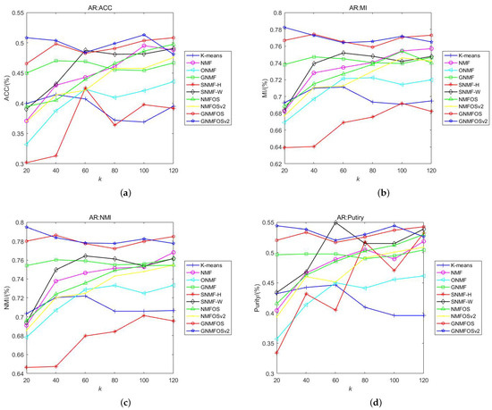
Figure 1. The clustering performance on AR. (a) ACC; (b) MI; (c) NMI; (d) Purity.

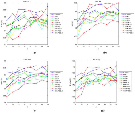
Figure 2. The clustering performance on ORL. (a) ACC; (b) MI; (c) NMI; (d) Purity.

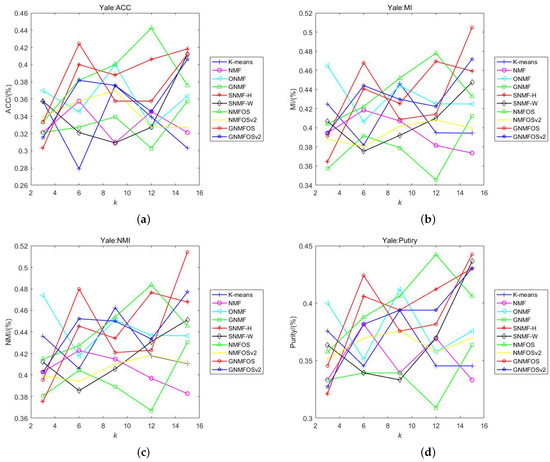
Figure 3. The clustering performance on Yale. (a) ACC; (b) MI; (c) NMI; (d) Purity.

Discussion of Results on AR Dataset:

• For indicators of ACC, MI, NMI, and Purity, GNMFOS achieves the highest values at the same clusters’ number $K=120$ in AR dataset, while GNMFOSv2 outperforms GONMF at other cluster numbers. Overall, GNMFOSv2 has the highest clustering indicator values.
• The differences in ACC, MI, NMI, and Purity, as well as their average values, for GNMFOS and GNMFOSv2 are not significant across different cluster numbers K. In contrast, most of other algorithms show larger fluctuations in clustering indicator values at different K. This shows that GNMFOS and GNMFOSv2 exhibit better stability across different cluster numbers, making them more suitable for applications.
• Among the orthogonal-based algorithms, ONMF, NMFOS, NMFOSv2, GNMFOS, and GNMFOSv2, the clustering performance of the proposed GNMFOS and GNMFOSv2 algorithms is the best. This indicates that our algorithms enhance the clustering performance and improve the sparse representation capability based on NMF methods.
• Among the graph Laplacian-based algorithms, GNMFOSv2 and GNMFOS consistently rank among the top two (followed by GNMF). This indicates that our models effectively utilize the hidden geometric structure information in data space.

Discussion of Results on ORL Dataset:

• When K is small (≤10), K-means achieves the highest values in ACC, MI, NMI, and Purity. When K is larger, the GNMFOS and GNMFOSv2 algorithms consistently rank among the top two in terms of the four clustering indicators. This shows that our algorithms are more suitable for larger numbers of clusters in the ORL dataset.
• Overall, GNMFOS has higher average values in ACC, MI, and Purity compared to GNMFOSv2 (NMI is slightly lower than GNMFOSv2), but the differences between GNMFOS and GNMFOSv2 are not significant. This indicates that, for the ORL dataset, GNMFOS is slightly more applicable.
• In terms of ACC, MI, NMI, and Purity, GNMFOS achieves the overall highest values at the same number of clusters $K=40$. This indirectly indicates that the GNMFOS algorithm is suitable for clustering the dataset into the original classes.
• Among the orthogonal-based algorithms (including ONMF, NMFOS, and NMFOSv2), GNMFOS and GNMFOSv2 exhibit the best clustering performance. This also indicates that our algorithms enhance the clustering performance and improve the sparse representation capability of NMF-based methods.
• Among the graph Laplacian-based algorithms including GNMF, GNMFOS and GNMFOSv2 exhibit the best clustering performance. This also indicates that our models effectively utilize the hidden geometric structure information in data space.

Discussion of Results on Yale Dataset:

• On the Yale dataset, no algorithm consistently leads in all four clustering indicators, so they need to be discussed separately. For ACC, NMFOS has the highest value (e.g., 0.4424 when $K=12$). However, it is worth noting that GNMFOS and GNMFOSv2 do not significantly lag behind NMFOS. Specifically, at $K=6$, GNMFOS achieves the second-highest rank. For MI, NMFOS also achieves the highest value, but GNMFOS lags behind it by only 0.04%, and GNMFOS attains the overall highest value at $K=15$, indicating strong competitiveness in MI. For NMI, GNMFOS has the highest value and achieves the overall highest value at $K=15$. For Purity, NMFOS has the highest value, but GNMFOS attains the overall highest values at $K=6$ and $K=15$, indicating that GNMFOS is also highly competitive.
• Although in some indicators, the values of NMFOS are slightly higher than those of GNMFOS and GNMFOSv2, these differences are moderate. The results indicate that both the GNMFOS and NMFOS algorithms are viable choices for the Yale dataset.
• For all four clustering indicators at $K=3$, ONMF has the highest values, indicating that the ONMF algorithm maybe more suitable for smaller K.
• When K increases, the values of ACC, MI, NMI, and Purity for NMFOS do not consistently increase or decrease monotonically. But for GNMFOS, the values of MI and NMI significantly increase. This indicates that our algorithms are more suitable for clustering experiments with larger numbers of clusters on the Yale dataset.
• The orthogonal-based algorithms (ONMF, NMFOS, NMFOSv2, GNMFOS, and GNMFOSv2) exhibit the overall best performance, indicating that algorithms with orthogonality are more suitable for the Yale dataset.

Overall, the algorithms proposed in this paper outperform algorithms that solely possess orthogonal, manifold, or sparse constraints. The results indicate that our algorithms successfully integrate the advantages of orthogonal constraints and geometric structures, further optimizing over the compared algorithms for a better learning of parts-based representation in the dataset. So, the above results demonstrate that our GNMFOS and GNMFOSv2 algorithms have strong competitiveness in clustering.

However, it is worth noting that no single algorithm consistently outperforms others across all four clustering indicators on the Yale dataset. This reflects the inherent trade-offs among different clustering evaluation metrics and highlights the limitations of current algorithms in achieving uniformly best performance. Such a phenomenon is common in clustering tasks where different metrics emphasize distinct aspects of clustering quality. Future work could focus on developing methods that balance multiple criteria more effectively.

4.4.2. Summary of Analysis on Image Datasets

In this part, we will summarize the above analysis on image datasets.

• In orthogonal-based algorithms, such as ONMF, NMFOS, NMFOSv2, GNMFOS, and GNMFOSv2, they outperform NMF, GNMF, SNMF-H, and SNMF-W algorithms on the Yale dataset. Moreover, on the AR and ORL datasets, GNMFOS and GNMFOSv2 exhibit the best clustering performance among them. In graph Laplacian-based algorithms, such as GNMF, GNMFOS, and GNMFOSv2, their clustering performance is almost superior to other algorithms. This is because graph-based algorithms consider local geometric structures, preserving locality in low-dimensional data space. The GNMFOS and GNMFOSv2 algorithms combine the advantages of orthogonality and graph, enhancing clustering performance and improving the sparse representation capability of NMF based models.
• Due to the various backgrounds in each dataset (e.g., lighting conditions, poses, etc.), the performances of GNMFOS and GNFOSv2 are different. For different feature dimensions, the values of ACC, MI, NMI, and Purity also show slight variations, but the overall performance of GNMFOS and GNFOSv2 remains stable.
• For the Yale dataset, GNMFOS and GNMFOSv2 do not significantly outperform, indicating that orthogonal penalty constraints and graph Laplacian constraints may not necessarily enhance clustering performance in certain situations. Therefore, further research is needed to develop more effective algorithms in the future.
• Considering the results for different clustering numbers K across the three image datasets, the clustering indicators (ACC, MI, NMI, and Purity) of the GNMFOS and GNMFOSv2 algorithms exhibit some fluctuations. However, overall, they outperform algorithms that only have orthogonal or manifold structure constraints, sparse constraints, or no constraints.

In conclusion, our algorithms demonstrate the best overall clustering performance for image datasets, and the above results have clearly shown that incorporating the orthogonality and graph regularity into the NMF model can enhance the clustering performance of the corresponding algorithms.

4.5. Clustering Results for Document Datasets

This subsection conducts clustering experiments on document datasets TDT2all and TDT2. In addition to the newly proposed GNMFOS and GNMFOSv2 models, the NMF, GNMF, NMFOS, and NMFOSv2 algorithms, which have shown excellent performance on image datasets, are selected for comparison. Similarly, detailed information on cluster numbers K is provided in the first column of Table 5 and Table 6. The tables consist of four sub-tables corresponding to four evaluation indicators, with the maximum values highlighted in bold. Adopting the same approach, we run tests separately for different cluster numbers and average the results over 10 runs. Details will be listed in Table 5 and Table 6. Figure 4 and Figure 5 display the corresponding line color images.

Table 5. The clustering performance on TDT2all.

Clusters K	NMF	GNMF	NMFOS	NMFOSv2	GNMFOS	GNMFOSv2
ACC
10	0.1806	0.3945	0.1703	0.1711	0.2919	0.2582
30	0.2401	0.3517	0.2391	0.2465	0.3851	0.3087
50	0.2771	0.3851	0.3168	0.2711	0.4227	0.4049
70	0.3038	0.3741	0.3290	0.3277	0.3840	0.3934
90	0.3437	0.3949	0.3234	0.3248	0.3829	0.4135
96	0.3131	0.3816	0.3223	0.3458	0.3835	0.4094
Avg.	0.2764	0.3803	0.2835	0.2811	0.3750	0.3647
MI
10	0.4433	0.5623	0.4273	0.4149	0.5217	0.5125
30	0.4823	0.5572	0.4816	0.4883	0.6068	0.5910
50	0.5119	0.5603	0.5125	0.4994	0.6211	0.6105
70	0.5197	0.5666	0.5210	0.5226	0.6001	0.6135
90	0.5395	0.5651	0.5323	0.5279	0.6081	0.6190
96	0.5246	0.5642	0.5377	0.5385	0.6105	0.6227
Avg.	0.5036	0.5626	0.5021	0.4986	0.5947	0.5949
NMI
10	0.5318	0.6570	0.5111	0.4950	0.6269	0.6140
30	0.5765	0.6526	0.5774	0.5825	0.7265	0.7133
50	0.6108	0.6578	0.6111	0.5954	0.7339	0.7333
70	0.6229	0.6649	0.6136	0.6235	0.7225	0.7356
90	0.6428	0.6647	0.6374	0.6260	0.7302	0.7411
96	0.6259	0.6659	0.6355	0.6442	0.7309	0.7456
Avg.	0.6018	0.6605	0.5977	0.5944	0.7118	0.7138
Purity
10	0.6817	0.8023	0.6645	0.6501	0.7714	0.7477
30	0.7380	0.7896	0.7389	0.7404	0.8866	0.8700
50	0.7659	0.8104	0.7789	0.7541	0.8929	0.8866
70	0.7770	0.8110	0.7725	0.7846	0.8838	0.8925
90	0.7916	0.8204	0.8065	0.7957	0.8846	0.9000
96	0.7818	0.8249	0.8050	0.8142	0.8897	0.9107
Avg.	0.7560	0.8098	0.7611	0.7565	0.8682	0.8679

Table 6. The clustering performance on TDT2.

Clusters K	NMF	GNMF	NMFOS	NMFOSv2	GNMFOS	GNMFOSv2
ACC
5	0.2482	0.6080	0.1947	0.2673	0.1947	0.3980
10	0.2912	0.6108	0.1947	0.3258	0.1947	0.4256
15	0.3719	0.5496	0.1947	0.3652	0.1947	0.4825
20	0.3562	0.6387	0.1947	0.3967	0.1947	0.5513
25	0.4044	0.5786	0.1947	0.4221	0.1947	0.5199
30	0.3587	0.6300	0.1947	0.4188	0.1947	0.6230
Avg.	0.3385	0.6026	0.1947	0.3660	0.1947	0.5001
MI
5	0.4330	0.6583	0.0019	0.4683	0.0019	0.6892
10	0.4884	0.6810	0.0019	0.5007	0.0019	0.7007
15	0.5204	0.6469	0.0019	0.5178	0.0019	0.6369
20	0.5373	0.6788	0.0019	0.5633	0.0019	0.6948
25	0.5737	0.6799	0.0019	0.5644	0.0019	0.6958
30	0.5550	0.6996	0.0019	0.5789	0.0019	0.7400
Avg.	0.5180	0.6741	0.0019	0.5322	0.0019	0.6929
NMI
5	0.4682	0.6878	0.0174	0.5143	0.0174	0.7309
10	0.5352	0.7077	0.0174	0.5511	0.0174	0.7648
15	0.5718	0.6739	0.0174	0.5663	0.0174	0.7029
20	0.5999	0.7251	0.0174	0.6121	0.0174	0.7597
25	0.6315	0.7025	0.0174	0.6173	0.0174	0.7384
30	0.6043	0.7217	0.0174	0.6297	0.0174	0.7956
Avg.	0.5685	0.7031	0.0174	0.5818	0.0174	0.7487
Purity
5	0.6137	0.7623	0.1977	0.6523	0.1977	0.7886
10	0.6652	0.7919	0.1977	0.6831	0.1977	0.8046
15	0.6622	0.7586	0.1977	0.7022	0.1977	0.8067
20	0.7261	0.8035	0.1977	0.7267	0.1977	0.8313
25	0.7330	0.7663	0.1977	0.7459	0.1977	0.8039
30	0.7193	0.7971	0.1977	0.7260	0.1977	0.8761
Avg.	0.6866	0.7799	0.1977	0.7060	0.1977	0.8185

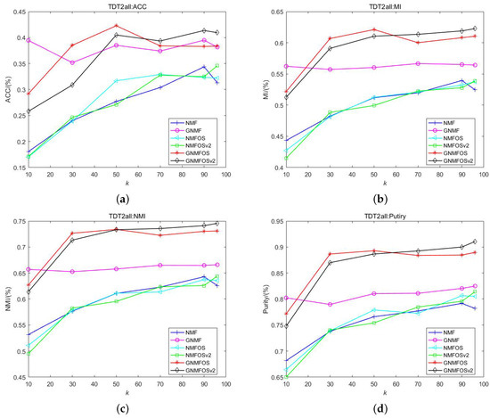
Figure 4. The clustering performance on TDT2all. (a) ACC; (b) MI; (c) NMI; (d) Purity.

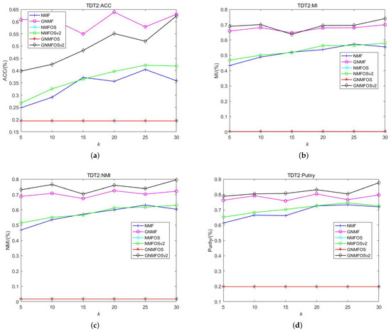
Figure 5. The clustering performance on TDT2. (a) ACC; (b) MI; (c) NMI; (d) Purity.

• For the TDT2all dataset, when $K\ge 70$, GNMFOSv2 achieves the maximum values in ACC, NMI, MI, and Purity; when $30\le K<70$, GNMFOS achieves the maximum values in ACC, NMI, MI, and Purity; when $K<30$, GNMF achieves the maximum values in ACC, NMI, MI, and Purity. Although GNMF has the best average performance in the ACC metric, GNMFOS, proposed in this paper, achieves the highest ACC value at $K=50$, reaching 42.27%. This suggests that GNMFOSv2 is more suitable when the number of clusters is close to the size of the document dataset itself; GNMFOS is more suitable when the number of clusters is moderate; and GNMF is more suitable when the number of clusters is very small. Additionally, GNMFOS ranks first in the average Purity indicator, while GNMFOSv2 ranks first in the average NMI and MI indicators.
• From Figure 4, it can be observed that, for the TDT2all dataset, the clustering performance is relatively optimal when the number of clusters K is set to 50. This suggests that the optimal number of clusters for the TDT2all dataset is 50. Additionally, the GNMF, GNMFOS, and GNMFOSv2 algorithms outperform the NMF, NMGOS, and NMFOSv2 algorithms significantly across all four indicators. This indicates that graph Laplacian-based algorithms can enhance clustering performance for the TDT2all document dataset.
• For the TDT2 dataset, the GNMFOSv2 algorithm achieves the best performance in terms of MI, NMI, and Purity across different numbers of clusters K and their average values. The GNMF algorithm performs better in terms of ACC; however, the ACC values of GNMFOSv2 increase as the number of clusters K increases. Particularly at $K=30$, the ACC value of GNMFOSv2 is only 0.7% lower than that of the GNMF algorithm. This indicates that when the number of clusters is close to the class structure of the document dataset itself, the GNMFOSv2 algorithm has significant potential in terms of ACC. Combining MI, NMI, and Purity, it can be concluded that the GNMFOSv2 algorithm is more suitable for the TDT2 document dataset when the number of clusters is relatively large.
• Additionally, it is worth nothing that the NMFOS and GNMGOS algorithms exhibit extremely low values in terms of ACC, NMI, MI, and Purity for the TDT2 dataset, and these values do not change with varying numbers of clusters K. This could be due to the zero-locking phenomenon mentioned earlier. In contrast, the NMFOSv2 and GNMFOSv2 algorithms incorporate $\delta$ into their iteration processes, preventing the zero-locking phenomenon. This suggests that the proposed GNMFOSv2 algorithm is practically significant, addressing issues observed in other algorithms.
• However, it is worth noting that no single algorithm consistently outperforms others across all four clustering indicators on the Yale dataset. This reflects the inherent trade-offs among different clustering evaluation metrics and highlights the limitations of current algorithms in achieving uniformly best performance. Such a phenomenon is common in clustering tasks where different metrics emphasize distinct aspects of clustering quality. Future work could focus on developing methods that balance multiple criteria more effectively.
• Considering the results of the two document datasets at different clustering numbers K, it can be concluded that the clustering indicators ACC, MI, NMI, and Purity of the GNMFOS and GNMFOSv2 algorithms exhibit some fluctuations, but overall, these algorithms outperform the other. Therefore, the proposed GNMFOS and GNMFOSv2 algorithms can effectively learn the parts-based representation of the dataset, making them effective for document clustering.

4.6. Parameter Sensitivity

We are now investigating how different choices of algorithm parameters will affect their numerical performance. Clearly, if an algorithm is not sensitive to different parameter choices, it can be considered more robust and easier to apply in practice. There are four parameters that affect the experimental results: the regularization parameter $\lambda$, the orthogonality parameter $\alpha$, the nearest neighbor point p, and the $\delta$ in Algorithm 2. So, in this subsection, we will compare the parameter choices of the GNMFOS and GNMFOSv2 algorithms.

Considering the comprehensiveness of the experiments, we first fix the nearest neighbor point p and $\delta$, and let $\alpha$ and $\lambda$ vary in $\left\{{10}^{-3},{10}^{-2},{10}^{-1},{10}^0,{10}^1,{10}^2,{10}^3\right\}$. Specifically, in the experiments, we set the parameters $\alpha$, $\lambda$ as a group for testing, and the experimental results are shown in Figure 6 and Figure 7.

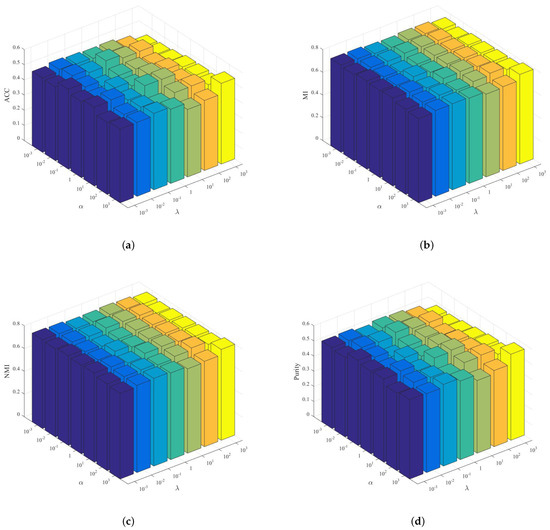
Figure 6. Performance variations in ACC, MI, NMI, and Purity with respect to different combinations of $\alpha$ and $\lambda$ values on AR dataset in GNMFOS. (a) ACC; (b) MI; (c) NMI; (d) Purity.

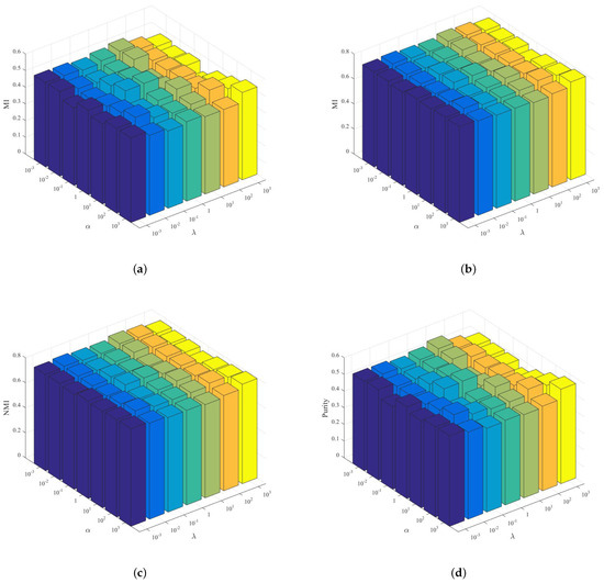
Figure 7. Performance variations in ACC, MI, NMI, and Purity with respect to different combinations of $\alpha$ and $\lambda$ values on AR dataset in GNMFOSv2. (a) ACC; (b) MI; (c) NMI; (d) Purity.

For the AR dataset, taking the number of classes in the dataset itself as the clustering number $K=120$, when the parameters $\alpha$, $\lambda$ are set to $\{1000,1000\}$, the clustering performance of the GNMFOS algorithm is relatively optimal. When the parameters $\alpha$, $\lambda$ are set to $\{1,1\}$, the clustering performance of the GNMFOSv2 algorithm is relatively optimal. At the same time, it can be observed that the clustering metrics of GNMFOS and GNMFOSv2 algorithms do not fluctuate much when the parameters $\alpha$ and $\lambda$ change. This indicates that these two algorithms are not sensitive to different parameter choices, making them more suitable for practical applications.

Then, based on Figure 6 and Figure 7, fixing the optimal parameters {$\alpha$, $\lambda$} = {1000, 1000} and {$\alpha$, $\lambda$} = {1,1} for GNMFOS and GNMFOSv2, respectively, we let the nearest neighbor point p vary in the range $\left\{1,3,5,7,9\right\}$. The experimental results are shown in Figure 8. It can be observed that for the AR dataset, the clustering performance of the GNMFOS algorithm is relatively optimal when the nearest neighbor point $p=3$. As we can see, the performance of GNMFOS is stable with respect to the parameters $\alpha$ and $\lambda$.

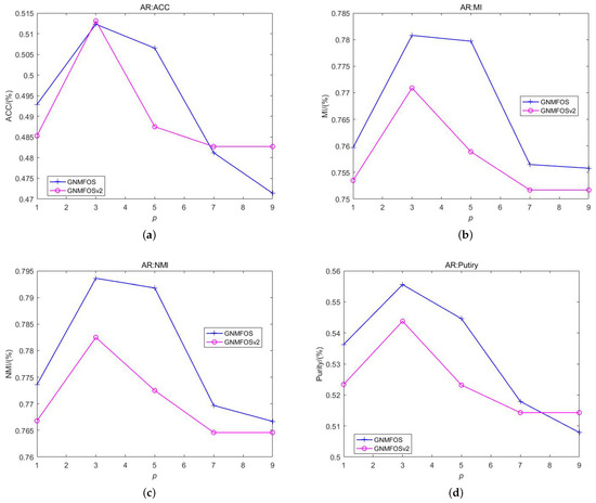
Figure 8. The performance of GNMFOS and GNMFOSv2 as p increases on AR dataset. (a) ACC; (b) MI; (c) NMI; (d) Purity.

However, it is important to note that GNMFOS and GNMFOSv2 rely on the assumption that two neighboring data points share the same label. Clearly, as p increases, this assumption may fail. This is also why the performance of GNMFOS and GNMFOSv2 decreases with increasing p. It demonstrates the existence of an optimal neighborhood size p for effectively learning the underlying manifold structures of the data.

Due to the fact that the parameter $\delta$ on the denominator of Algorithm 2’s MUR cannot be too large, as it might affect the convergence of finer rules, we uniformly set it to $1\times {10}^{-8}$.

Considering the overall results, the performance of the GNMFOS and GNMFOSv2 algorithms is highly robust to different values of parameters $\lambda$, $\alpha$, and p. The algorithm exhibits stability even across a wide range of parameter values, demonstrating its ability to capture both global and local geometric structures effectively and showcasing good generalization ability. The following bar charts demonstrate the robustness of our new algorithms well, and the subsequent line graphs in Figure 8 also illustrate the conclusion that the parameter p is also robust.

4.7. Weighting Scheme Selection

There are several choices for defining the weight matrix S on the p-nearest neighbors. Three popular schemes are 0-1 weighting, heat kernel weighting, and dot product weighting. In our previous experiments, for simplicity, we used 0-1 weighting, where, for a given point x, the p-nearest neighbors are treated as equally important. However, in many cases, it is necessary to distinguish these p nearest neighbors, especially when p is large. In such cases, heat kernel weighting or dot product weighting can be used [15].

For image data, Figure 9 and Figure 10 illustrate the relationship between the clustering performance of the GNMFOS algorithm and that of the GNMFOSv2 algorithm on the AR dataset as the number of nearest neighbors p varies. The cluster number is set to 120, matching the number of classes in the dataset. It can be observed that for the GNMFOSv2 algorithm, different values of p correspond to different optimal schemes. This variation might be attributed to the impact of the parameter $\delta$ in the update rule of the algorithm. The optimal weighting scheme can be chosen based on practical considerations.

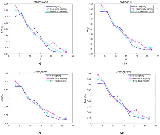
Figure 9. The performance of GNMFOS and with different weighting schemes on AR dataset. (a) ACC; (b) MI; (c) NMI; (d) Purity.

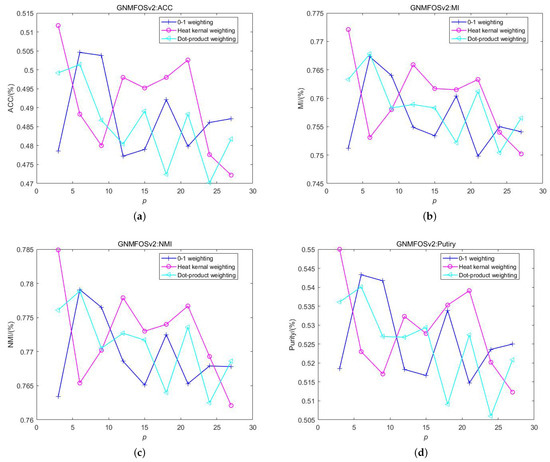
Figure 10. The performance of GNMFOSv2 and with different weighting schemes on AR dataset. (a) ACC; (b) MI; (c) NMI; (d) Purity.

For the GNMFOS algorithm, the heat kernel scheme is superior to the 0-1 weighting scheme and the dot product weighting scheme when $p\le 10$. When $10\le p\le 15$, the 0-1 weighting scheme is optimal, and when $p\ge 15$, the heat kernel scheme is optimal. However, the heat kernel scheme involves a parameter $\sigma$, which is crucial for this scheme. Automatically selecting the parameter $\sigma$ is a challenging problem that has garnered significant interest among researchers.

For document data, document vectors are often normalized to unit vectors. In this case, the dot product of two document vectors becomes their cosine similarity, a widely used document similarity metric in the information retrieval community. Therefore, using dot product weighting is common for document data. Unlike the 0-1 weighting, the dot product weighting does not involve any parameters.

Figure 11 and Figure 12 illustrate the relationship between the clustering performance of the GNMFOSv2 algorithm with 0-1 weighting and dot product weighting schemes on the TDT2all document dataset as the number of nearest neighbors p varies. The cluster number is set to 96, matching the number of classes in the dataset. It can be observed that for the GNMFOS algorithm, the dot product weighting scheme performs better, especially when p is large. For the GNMFOSv2 algorithm, the 0-1 weighting scheme exhibits significant fluctuations. Specifically, at $p=12$ and $p=21$, the values of the four clustering metrics are low, while at $p=15$, the values are high. However, at $p=3$, the clustering performance is optimal. Overall, the 0-1 weighting scheme is more suitable for the GNMFOSv2 algorithm.

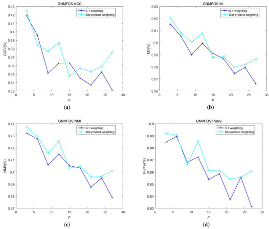
Figure 11. The performance of GNMFOS and with different weighting schemes on TDT2all dataset. (a) ACC; (b) MI; (c) NMI; (d) Purity.

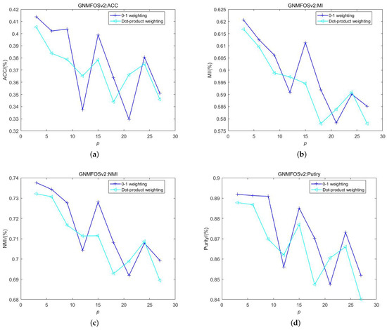
Figure 12. The performance of GNMFOSv2 and with different weighting schemes on TDT2all dataset. (a) ACC; (b) MI; (c) NMI; (d) Purity.

5. Conclusions

Two effective algorithms are developed to solve the proposed model, and more importantly, their convergence has been theoretically proven.

The main contributions of this work are summarized as follows:

• GNMFOS integrates the strengths of both NMFOS and GNMF by incorporating orthogonality constraints and a graph Laplacian term into the objective function. This enhances the model’s capability in sparse representation, reduces computational complexity, and improves clustering accuracy by leveraging the underlying geometric structure of both data and feature spaces.
• The model supports flexible control over orthogonality and regularization through parameters $\alpha$ and $\lambda$, respectively. This makes GNMFOS adaptable to various real-world scenarios.
• Extensive experiments on three image datasets and two document datasets demonstrate the superior clustering performance of GNMFOS and its variant GNMFOSv2. The image experiments show better parts-based feature learning and higher discriminative power, while the document experiments suggest improved semantic structure representation.

In future work, we aim to apply GNMFOS to data from diverse fields such as medicine, engineering, and management to further validate its effectiveness. In addition, considering the inherent complexity of NMF-based optimization models, developing more efficient algorithms for large-scale and constrained scenarios remains an important research direction.

References

- Devarajan, K. Nonnegative matrix factorization: An analytical and interpretive tool in computational biology. PLoS Comput. Biol. 2008, 4, e1000029. [Google Scholar] [CrossRef] [PubMed]
- Gao, Z.; Wang, Y.T.; Wu, Q.W.; Ni, J.C.; Zheng, C.H. Graph regularized l2, 1-nonnegative matrix factorization for mirna-disease association prediction. BMC Bioinform. 2020, 21, 1–13. [Google Scholar] [CrossRef] [PubMed]
- Zhang, L.; Liu, Z.; Pu, J.; Song, B. Adaptive graph regularized nonnegative matrix factorization for data representation. Appl. Intell. 2020, 50, 438–447. [Google Scholar] [CrossRef]
- Gillis, N.; Glineur, F. A multilevel approach for nonnegative matrix factorization. J. Comput. Appl. Math. 2012, 236, 1708–1723. [Google Scholar] [CrossRef]
- Hoyer, P.O. Non-negative matrix factorization with sparseness constraints. J. Mach. Learn. Res. 2002, 5, 457–469. [Google Scholar]
- Wang, D.; Lu, H. On-line learning parts-based representation via incremental orthogonal projective non-negative matrix factorization. Signal Process. 2013, 93, 1608–1623. [Google Scholar] [CrossRef]
- Berry, M.W.; Browne, M.; Langville, A.N.; Pauca, V.P.; Plemmons, R.J. Algorithms and applications for approximate nonnegative matrix factorization. Comput. Stat. Data Anal. 2007, 52, 155–173. [Google Scholar] [CrossRef]
- Pauca, V.P.; Piper, J.; Plemmons, R.J. Nonnegative matrix factorization for spectral data analysis. Linear Algebra Its Appl. 2006, 416, 29–47. [Google Scholar] [CrossRef]
- Bertin, N.; Badeau, R.; Vincent, E. Enforcing harmonicity and smoothness in bayesian non-negative matrix factorization applied to polyphonic music transcription. IEEE Trans. Audio Speech Lang. Process. 2010, 18, 538–549. [Google Scholar] [CrossRef]
- Zhou, G.; Yang, Z.; Xie, S.; Yang, J.M. Online blind source separation using incremental nonnegative matrix factorization with volume constraint. IEEE Trans. Neural Netw. 2023, 22, 550–560. [Google Scholar] [CrossRef] [PubMed]
- Fan, F.; Jing, P.; Nie, L.; Gu, H.; Su, Y. SADCMF: Self-Attentive Deep Consistent Matrix Factorization for Micro-Video Multi-Label Classification. IEEE Trans. Multimed. 2024, 26, 10331–10341. [Google Scholar] [CrossRef]
- Chen, D.; Li, S.X. An augmented GSNMF model for complete deconvolution of bulk RNA-seq data. Math. Biosci. Eng. 2025, 22, 988. [Google Scholar] [CrossRef] [PubMed]
- Xi, L.; Li, R.; Li, M.; Miao, D.; Wang, R.; Haas, Z. NMFAD: Neighbor-aware mask-filling attributed network anomaly detection. IEEE Trans. Inf. Forensics Secur. 2024, 20, 364–374. [Google Scholar] [CrossRef]
- Chen, X.; Wang, J.; Huang, Q. Dynamic Spectrum Cartography: Reconstructing Spatial-Spectral-Temporal Radio Frequency Map via Tensor Completion. IEEE Trans. Signal Process. 2025, 73, 1184–1199. [Google Scholar] [CrossRef]
- Cai, D.; He, X.; Han, J.; Huang, T.S. Graph regularized nonnegative matrix factorization for data representation. IEEE Trans. Pattern Anal. Mach. Intell. 2010, 33, 1548–1560. [Google Scholar] [CrossRef] [PubMed]
- Hu, W.; Choi, K.S.; Wang, P.; Jiang, Y.; Wang, S. Convex nonnegative matrix factorization with manifold regularization. Neural Netw. 2015, 63, 94–103. [Google Scholar] [CrossRef] [PubMed]
- Meng, Y.; Shang, R.; Jiao, L.; Zhang, W.; Yuan, Y.; Yang, S. Feature selection based dual-graph sparse non-negative matrix factorization for local discriminative clustering. Neurocomputing 2018, 290, 87–99. [Google Scholar] [CrossRef]
- Long, X.; Lu, H.; Peng, Y.; Li, W. Graph regularized discriminative non-negative matrix factorization for face recognition. Multimed. Tools Appl. 2014, 72, 2679–2699. [Google Scholar] [CrossRef]
- Shang, F.; Jiao, L.; Wang, F. Graph dual regularization non-negative matrix factorization for co-clustering. Pattern Recognit. 2012, 45, 2237–2250. [Google Scholar] [CrossRef]
- Che, H.; Li, C.; Leung, M.; Ouyang, D.; Dai, X.; Wen, S. Robust hypergraph regularized deep non-negative matrix factorization for multi-view clustering. IEEE Trans. Emerg. Top. Comput. Intell. 2025, 9, 1817–1829. [Google Scholar] [CrossRef]
- Yang, X.; Che, H.; Leung, M.; Liu, C.; Wen, S. Auto-weighted multi-view deep non-negative matrix factorization with multi-kernel learning. IEEE Trans. Signal Inf. Pract. 2025, 11, 23–34. [Google Scholar] [CrossRef]
- Liu, C.; Li, R.; Che, H.; Leung, M.F.; Wu, S.; Yu, Z.; Wong, H.S. Beyond euclidean structures: Collaborative topological graph learning for multiview clustering. IEEE Trans. Neural Netw. Learn. Syst. 2025, 36, 10606–10618. [Google Scholar] [CrossRef] [PubMed]
- Li, G.; Zhang, X.; Zheng, S.; Li, D. Semi-supervised convex nonnegative matrix factorizations with graph regularized for image representation. Neurocomputing 2017, 237, 1–11. [Google Scholar] [CrossRef]
- Li, S.Z.; Hou, X.W.; Zhang, H.J.; Cheng, Q.S. Learning spatially localized, parts-based representation. In Proceedings of the 2001 IEEE Computer Society Conference on Computer Vision and Pattern Recognition, CVPR 2001, Kauai, HI, USA, 8–14 December 2001. [Google Scholar]
- Ding, C.; Li, T.; Peng, W.; Park, H. Orthogonal nonnegative matrix t-factorizations for clustering. In Proceedings of the 12th ACM SIGKDD International Conference on Knowledge Discovery and Data Mining, Philadelphia, PA, USA, 20–23 August 2006; pp. 126–135. [Google Scholar]
- Li, S.; Li, W.; Hu, J.; Li, Y. Semi-supervised bi-orthogonal constraints dual-graph regularized nmf for subspace clustering. Appl. Intell. 2022, 52, 227–3248. [Google Scholar] [CrossRef]
- Liang, N.; Yang, Z.; Li, Z.; Han, W. Incomplete multi-view clustering with incomplete graph-regularized orthogonal non-negative matrix factorization. Appl. Intell. 2022, 52, 14607–14623. [Google Scholar] [CrossRef]
- Zhang, X.; Xiu, X.; Zhang, C. Structured joint sparse orthogonal nonnegative matrix factorization for fault detection. IEEE Trans. Instrum. Meas. 2023, 72, 1–15. [Google Scholar] [CrossRef]
- Lee, D.D.; Seung, H.S. Learning the parts of objects by non-negative matrix factorization. Nature 1999, 401, 788–791. [Google Scholar] [CrossRef] [PubMed]
- Li, Z.; Wu, X.; Peng, H. Nonnegative matrix factorization on orthogonal subspace. Pattern Recognit. Lett. 2010, 31, 905–911. [Google Scholar] [CrossRef]
- Peng, S.; Ser, W.; Chen, B.; Sun, L.; Lin, Z. Robust nonnegative matrix factorization with local coordinate constraint for image clustering. Eng. Appl. Artif. Intell. 2020, 88, 103354. [Google Scholar] [CrossRef]
- Tosyali, A.; Kim, J.; Choi, J.; Jeong, M.K. Regularized asymmetric nonnegative matrix factorization for clustering in directed networks. Pattern Recognit. Lett. 2019, 125, 750–757. [Google Scholar] [CrossRef]
- Guo, J.; Wan, Z. A modified spectral prp conjugate gradient projection method for solving large-scale monotone equations and its application in compressed sensing. Math. Probl. Eng. 2019, 2019, 5261830. [Google Scholar] [CrossRef]
- Li, T.; Wan, Z. New adaptive barzilai–borwein step size and its application in solving large-scale optimization problems. ANZIAM J. 2019, 61, 76–98. [Google Scholar]
- Lv, J.; Deng, S.; Wan, Z. An efficient single-parameter scaling memoryless broyden-fletcher-goldfarb-shanno algorithm for solving large scale unconstrained optimization problems. IEEE Access 2020, 8, 85664–85674. [Google Scholar] [CrossRef]
- Mirzal, A. A convergent algorithm for orthogonal nonnegative matrix factorization. J. Comput. Appl. Math. 2014, 260, 149–166. [Google Scholar] [CrossRef]
- Wang, J.; Wang, J.; Ke, Q.; Zeng, G.; Li, S. Fast approximate k-means via cluster closures. In Multimedia Data Mining and Analytics: Disruptive Innovation; Springer: Berlin/Heidelberg, Germany, 2015; pp. 373–395. [Google Scholar]
- Hoyer, P.O. Non-negative sparse coding. In Proceedings of the 12th IEEE Workshop on Neural Networks for Signal Processing, Martigny, Switzerland, 6 September 2002; pp. 557–565. [Google Scholar]
- Lee, D.D.; Seung, H.S. Algorithms for non-negative matrix factorization. Adv. Neural Inf. Process. Syst. 2000, 13, 535–541. [Google Scholar]
Disclaimer/Publisher’s Note: The statements, opinions and data contained in all publications are solely those of the individual author(s) and contributor(s) and not of MDPI and/or the editor(s). MDPI and/or the editor(s) disclaim responsibility for any injury to people or property resulting from any ideas, methods, instructions or products referred to in the content. |
© 2025 by the authors. Licensee MDPI, Basel, Switzerland. This article is an open access article distributed under the terms and conditions of the Creative Commons Attribution (CC BY) license (https://creativecommons.org/licenses/by/4.0/).