Fault Diagnosis Method for Pumped Storage Units Based on VMD-BILSTM

Abstract

The construction of pumped storage power stations (PSPSs) is undergoing rapid expansion globally. Detecting operational faults and defects in pumped storage units is critical, as effective diagnostic methods can not only identify fault types quickly and accurately but also significantly reduce maintenance costs. This study leverages the symmetry characteristics in the vibration signals of pumped storage units to enhance fault diagnosis accuracy. To address the challenges of selecting the key parameters (e.g., decomposition level and penalty factor) of the variational mode decomposition (VMD) algorithm during vibration signal analysis, this paper proposes an algorithm for an improved subtraction-average-based optimizer (ISABO). By incorporating piecewise linear mapping, the ISABO enhances parameter initialization and, combined with a balanced pool method, mitigates the algorithm’s tendency to converge to local optima. This improvement enables more effective vibration signal denoising and feature extraction. Furthermore, to optimize hyperparameter selection in the bidirectional long short-term memory (BILSTM) network—such as the number of hidden layer units, maximum training epochs, and learning rate—we introduce an ISABO-BILSTM classification model. This approach ensures robust fault diagnosis by fine-tuning the neural network’s critical parameters. The proposed method is validated using vibration data from an operational PSPS. Experimental results demonstrate that the ISABO-BILSTM model achieves an overall fault recognition accuracy of 97.96%, with the following breakdown: normal operation: 96.29%, thrust block loosening: 98.60%, rotor-stator rubbing: 97.34%, and rotor misalignment: 99.59%. These results confirm that the proposed framework significantly improves fault identification accuracy, offering a novel and reliable approach for PSPS unit diagnostics.

1. Introduction

The concept of symmetry plays a fundamental role in mechanical system dynamics. For rotating machinery such as pumped storage units, symmetry-breaking phenomena often precede observable faults, which holds significant practical implications for fault diagnosis implementation. Pumped storage units serve as the central facilities in pumped storage power stations, where equipment failures may jeopardize the operational safety and stability of the power station, potentially compromising grid stability. Moreover, studies have indicated that the vast majority of faults in pumped storage units manifest directly or indirectly through mechanical vibrations. Therefore, conducting systematic research on the vibration signals of pumped storage units is of significant value for ensuring the safe and stable operation of these critical electromechanical systems [1].

Currently, time-frequency analysis methods such as wavelet transform, empirical mode decomposition (EMD), and variational mode decomposition (VMD) have been extensively applied in vibration signal processing. Wavelet transform extends the Fast Fourier Transform (FFT) by incorporating an adaptive window adjustment mechanism, demonstrating superior adaptability in extracting features from non-stationary vibration signals [2]. Building upon wavelet transform, researchers initially proposed wavelet threshold denoising algorithms. Subsequent enhanced variants of wavelet threshold-based methods have emerged and demonstrated notable success in vibration signal processing and noise reduction for rotating machinery [3,4,5]. Empirical mode decomposition (EMD), proposed by Huang et al. [6], is distinguished by its adaptive time-frequency analysis capability for nonlinear and non-stationary signals and has been widely adopted in the field of signal processing [7,8,9]. In Reference [10], the authors integrated empirical mode decomposition (EMD) with independent component analysis (ICA) for signal denoising, and simulation experiments validated the efficacy of the proposed model. Variational mode decomposition (VMD), proposed by K. Dragomiretskiy et al. [11], is a novel adaptive signal decomposition method. Rooted in variational principles, this technique demonstrates exceptional precision and computational efficiency while effectively mitigating boundary effects—a common challenge in traditional decomposition methods [12,13,14]. Li et al. [12] leveraged the near-perfect reconstruction criterion to precisely identify bearing fault features, thereby addressing the detection challenges of incipient weak faults under strong ambient noise. Ding et al. [15] employed the variance of the autocorrelation function as a screening criterion to select the intrinsic mode functions (IMFs) after VMD, thereby accurately distinguishing between noise components and signal components. However, the noise reduction performance of the VMD method is affected by the number of modes and the penalty factor [16]. Currently, the selection of these two parameters primarily relies on empirical human judgment, thus necessitating further optimization of their determination methods. Huang et al. [17] employed the scale-space method to determine the number of modes in the processing of bearing vibration signals. Zhao et al. [18] determined the two parameters by using envelope nesting and a multi-criterion objective function, respectively. Simulation experiments verified the effectiveness of the proposed methods.

Currently, intelligent learning algorithms based on machine learning and deep learning technologies have been widely applied in the field of mechanical equipment fault diagnosis [19]. Maulik S. et al. [20] employed a random forest algorithm to identify faults in three-phase induction motors. During the feature extraction stage, they integrated features from both vibration and current signals, thereby further enhancing the model’s recognition accuracy. Cao H. et al. [21] redefined the joint objective function to balance different parameter losses. The proposed novel, unsupervised domain adversarial network diagnostic model demonstrated advantages over its counterparts. Hong G. et al. [22] utilized Mel spectrograms for data analysis and combined autoencoders with K-means for classification and recognition. Experiments showed that their model was more accurate compared to SVM, CNN-SVM, and DAE. Wan L. [23] employed wavelet packet decomposition in the feature extraction stage and optimized the K-means clustering algorithm using the ant colony optimization algorithm for the classification model. Experiments demonstrated that the proposed method exhibited superior diagnostic accuracy and efficiency. Rahimilarki R. et al. [24] applied time series analysis and convolutional neural networks (CNNs) to the fault diagnosis of wind turbines and validated the proposed method using fault data, which showed high diagnostic accuracy. Many models have been developed based on CNNs, such as Le Net, Alex Net, and VGG Net [25]. Shi X. et al. [26] proposed a fault diagnosis method combining variational mode decomposition (VMD) and the Alex Net model, which achieved higher diagnostic accuracy than traditional convolutional neural networks. Zou et al. [27] combined multi-scale weighted entropy morphological filtering with bidirectional long short-term memory (BILSTM) to address the issues of low distinguishability of intrinsic mode functions and high computational complexity in traditional methods. The classification accuracy of the BILSTM reached 99%.

Although the aforementioned methods have achieved improvements in diagnostic accuracy, they suffer from a large number of adjustable parameters and a tendency to fall into local optima. In light of these issues, this paper proposes an improved version of the subtraction-average-based optimizer (SABO) as the subsequent parameter optimization algorithm. The improved SABO is employed to optimize the parameters of variational mode decomposition (VMD) for signal denoising and feature extraction. Furthermore, a bidirectional long short-term memory (BILSTM) network is utilized to accurately identify faults. This approach effectively addresses the problems of numerous adjustable parameters and cumbersome operations associated with traditional diagnostic methods. It offers a novel method for the fault diagnosis of pumped storage units. The effectiveness of the proposed model is validated using data collected from a pumped storage power station.

The main contributions of this paper are as follows: (1) The vibration signal of a pumped storage unit is decomposed using VMD. Piecewise linear chaotic mapping is combined with the equilibrium pool embedding method and an improved subtractive optimizer algorithm to optimize the penalty factor and the number of decomposition layers in VMD. After decomposition, sample entropy is used to denoise the vibration signal. The simulation signal is established in MATLAB, and the experiment shows that the signal denoising model established in this paper using the ISABO for optimization of VMD parameters can handle non-stationary signals well and has good adaptability to the actual signals of pumped storage units. (2) To address the problem of diagnostic performance being affected by the improper adjustment of relevant parameters in the bidirectional long short-term memory network, an improved subtraction-average-based optimizer (ISABO) algorithm is proposed to optimize the three parameters affecting the accuracy of the BILSTM: the number of the implicit layer units, the maximum training period, and the selection of the learning rate. Based on this, an ISABO-BILSTM classification model is constructed for fault diagnosis.

2. Fundamental Theory

2.1. Variational Mode Decomposition

The VMD algorithm decomposes non-stationary signal sequences into a set of mode functions with finite bandwidth by seeking the optimal solution to a constrained variational problem [28]. The specific steps are as follows:

Firstly, the original signal $f\left(t\right)$ is decomposed into K modal components ${\mu }_k\left(t\right)$. The energy spectrum is obtained through the Hilbert transform. The equality of $f\left(t\right)$ and the sum of all modal components ${\mu }_k\left(t\right)$ is used as a constraint condition. A Lagrange multiplier $\lambda \left(t\right)$ and a penalty factor $\alpha$ are introduced to transform the problem into a variational problem, as shown in Equation (1).

$$\left\{\begin{array}{l}\underset{\left\{{\mu }_k\right\}\left\{{\omega }_k\right\}}{\min }\left\{{{\displaystyle \sum _k^K‖{\mathsf{\partial }}_t[(\delta (t)+\frac{j}{\pi t})\ast {\mu }_k(t)]e^{-j{\omega }_{k}t}‖}}_2^2\right\}\\ \underset{{\mu }_k,{\omega }_k\lambda }{L}=\alpha {{\displaystyle \sum _k^K‖{\mathsf{\partial }}_t[(\delta (t)+\frac{j}{\pi t})\ast {\mu }_k(t)]e^{-j{\omega }_{k}t}‖}}_2^2+{‖f(t)-{\displaystyle \sum _{k=1}^K{\mu }_k(t)}‖}_2^2+⟨\lambda (t),f(t)-{\displaystyle \sum _{k=1}^K{\mu }_k(t)}⟩\end{array}\right.$$

(1)

In the equation, $*$ denotes the convolution operation, ${\mu }_k\left(t\right)$ represents the K-th modal component, ${\omega }_k$ is the center frequency, $\delta \left(t\right)$ is the Dirac delta function, ${\mathsf{\partial }}_t$ indicates the partial derivative with respect to ‘t’, and $⟨\lambda (t),f(t)-{\displaystyle \sum _{k=1}^K{\mu }_k(t)}⟩$ represents the inner product. The Alternating Direction Method of Multipliers (ADMM) is employed to solve the variational problem and obtain the optimal ${\mu }_k\left(t\right)$ and ${\omega }_k$. The specific implementation steps are as follows:

(1)

Initialize the parameters ${\mu }_k\left(t\right)$, ${\omega }_k$ and $\lambda$, set the iteration loop $n=n+1$, and update the parameters iteratively according to Equations (2) and (3).

(2)

Update ${\mu }_k(t)$.

$${\widehat{\mu }}_k^{n+1}(\omega )={\displaystyle \frac{\widehat{f}(\omega )-{\displaystyle \sum _{i=1}^{k-1}{\widehat{\mu }}^n(\omega )+\frac{{\widehat{\lambda }}^n(\omega )}{2}}}{1+2\alpha {(\omega -{\omega }_k^n)}^2}}$$

(2)

(3)

Update ${\omega }_k$.

$${\omega }_k^{n+1}={\displaystyle \frac{{\displaystyle {\int }_0^{\infty }\omega {\left|{\widehat{\mu }}_k^{n+1}(\omega )\right|}^{2}d\omega }}{{\displaystyle {\int }_0^{\infty }{\left|{\widehat{\mu }}_k^{n+1}(\omega )\right|}^{2}d\omega }}}$$

(3)

(4)

Update $\lambda$.

$${\widehat{\lambda }}^{n+1}={\widehat{\lambda }}^n+\tau [\widehat{f}(\omega )-{\displaystyle \sum _{k=1}^K{\widehat{\mu }}_k^{n+1}(\omega )}]$$

(4)

(5)

Convergence determination.

$${\displaystyle \frac{{\displaystyle \sum _{k=1}^K{‖{\widehat{\mu }}_k^{n+1}-{\widehat{\mu }}_k^n‖}_2^2}}{{‖{\widehat{\mu }}_k^{n+1}‖}_2^2}}<\varsigma$$

(5)

(6)

Check whether the iteration condition is satisfied; otherwise, return to step (2).

2.2. Subtractive Average Optimizer Improved by Multiple Strategies

In 2023, Mohammad proposed the subtraction-average-based optimizer (SABO) algorithm [29]. This algorithm is based on mathematical concepts and updates the positions of population members in the search space using the subtraction average of individuals. It demonstrates good performance in parameter optimization and function solving.

In the process of solving optimization problems, the search space boundaries are typically defined to constrain the population size. The population in the algorithm can be represented as a matrix, as shown in Equation (6), while the initialization of individual positions within the search space is primarily governed by Equation (7).

$$X=\left[\begin{array}{c}{X}_1\\ ⋮\\ X_i\\ ⋮\\ X_N\end{array}\right]=\left[\begin{array}{ccccc}{x}_{1,1}& \dots & x_{1,d}& \dots & x_{1,m}\\ ⋮& \ddots & ⋮& ⋰& ⋮\\ x_{i,1}& \dots & x_{i,d}& \dots & x_{i,m}\\ ⋮& ⋰& ⋮& \ddots & ⋮\\ x_{N,1}& \dots & x_{N,d}& \dots & x_{N,m}\end{array}\right]$$

(6)

$$x_{i,d}=l{b}_d+r_{i,d}\cdot \left(u{b}_d-l{b}_d\right),i=1,\dots ,N,d=1,\dots ,m$$

(7)

In the formula, X represents the overall matrix of the SABO, while $X_i$ denotes the i-th individual. $d$ indicates the dimension of the individuals in the search space. $N$ represents the number of individuals, and $m$ signifies the number of decision variables. $r_{i,d}$ is a random number within the interval [0, 1], and ub_d and lb_d denote the lower and upper bounds of the d-th decision variable, respectively.

Each search particle represents a possible solution to the problem, offering candidate values for decision variables. The objective function values are denoted by vector $\overrightarrow{F}$, as per Equation (8).

$$\overrightarrow{F}={\left[\begin{array}{c}{F}_1\\ ⋮\\ F_i\\ ⋮\\ F_N\end{array}\right]}_{N\times 1}={\left[\begin{array}{c}F\left(X_1\right)\\ ⋮\\ F\left(X_i\right)\\ ⋮\\ F\left(X_N\right)\end{array}\right]}_{N\times 1}$$

(8)

Here $\overrightarrow{F}$ is the vector of objective function values, and $F_i$ is the evaluated value for the objective function based on the i-th search agent.

The objective function values effectively gauge solution quality proposed by search agents. The best and worst values correspond to the top and bottom agents, respectively. As agent positions update per iteration, the process of identifying and retaining the best agent persists till the algorithm concludes.

The SABO algorithm utilizes the collective intelligence of the population during its search process. While its parameter configuration is relatively straightforward, its optimization performance may be affected by the initial population distribution. Insufficient coverage of the search space by the initial population could lead to convergence to local optima. Moreover, when generating new individuals, the algorithm only considers the current iteration’s individual positions without accounting for the iteration’s optimal solution. To enhance the optimization capability of the subtractive optimizer, this study employs piecewise linear chaotic mapping to improve the initial population distribution across the search space. Additionally, the integrated equilibrium pool mechanism is introduced to prevent positional deviation of the optimal solution during iterations, thereby avoiding premature convergence to local optima. The specific improvements are detailed as follows:

(1)

Piecewise Linear Chaotic Map

To ensure a more uniform and natural distribution of initial positions during the optimization algorithm’s initialization phase, this study replaces the SABO’s original random initialization process with a piecewise linear chaotic map (PWLCM). This modification enhances search space diversity and improves the algorithm’s optimization performance, as expressed in Equation (9).

The parameter $p$ determines non-overlapping ranges in the four-segment piecewise function, with $p=0.4$ adopted in this study. $r$ represents the randomly generated number within [0, 1] after chaotic transformation. The computational expression for population initialization using chaotic mapping is updated, as shown in Equation (10).

The population initialization was performed using both random distribution and piecewise linear chaotic mapping, respectively. Figure 1 illustrates the initial population distributions generated by these two methods. When employing a PWLCM, the initial individuals demonstrate a more natural and uniform distribution across the search space, exhibiting enhanced randomness that better represents the ideal initial population state. This approach effectively resolves the issues of local clustering and void regions that may occur during random initialization processes.

$$r_{i+1}=\left\{\begin{array}{l}{\displaystyle \frac{r_i}{p}},p\le r_i<p\\ {\displaystyle \frac{r_i-p}{0.5-p}},p\le r_i<0.5\\ {\displaystyle \frac{1-p-r_i}{0.5-p}},0.5\le r_i<1-p\\ {\displaystyle \frac{1-r_i}{p}},1-p\le r_i<1\end{array}\right.$$

(9)

$$x_{i,d}=l{b}_d+x_{i+1}\cdot \left(u{b}_d-l{b}_d\right)$$

(10)

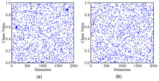
Figure 1. Comparison of the initial populations of different methods: (a) random initialization and (b) chaotic map initialization.

In MATLAB R2021a, according to the data sets of two initialized populations, the autocorrelation coefficient, the maximum and minimum distance ratios, and the degree of discrepancy are calculated, and the results are shown in Table 1. It can be seen from the data in Table 1 that the autocorrelation coefficient of the PWLCM is 0.0135, which is closer to 0 than that of the randomly initialized population, indicating that it is more random and disordered. The maximum and minimum distance ratios and the degree of discrepancy of the PWLCM are 0.9654 and 0.0259, respectively. The variances are 0.9654 and 0.0259, respectively, which is more advantageous in terms of uniformity than the randomly generated initialized population.

Table 1. Performance comparison of different initialization methods.

Evaluation Indicators	Random Initialization	Chaotic Map Initialization
Autocorrelation Coefficient	0.0238	0.0135
Max-Min Ratio	0.9426	0.9654
Discrepancy	0.0307	0.0259

(2)

Proposed Equilibrium Pool Embedding Mechanism

To address the tendency of optimization algorithms to converge to local optima during the search process, this study incorporates an equilibrium pool method. The approach replaces the current best solution with a randomly selected individual from the pool, employing a uniform probability distribution during the selection process. This mechanism updates the optimal solution’s position while enhancing population diversity, thereby facilitating escape from local optima.

The mathematical model of the equilibrium pool is presented in Equation (11). The position update process incorporating the embedded equilibrium pool is formulated in Equation (12).

$$X_{\mathrm{eq}}=\left\{X_{\mathrm{eq}1},X_{\mathrm{eq}2},X_{\mathrm{eq}3},X_{\mathrm{eq}4},X_{\mathrm{eqave}}\right\}$$

(11)

$$X_i^{new}=X_{\mathrm{eq}}+{\overrightarrow{r}}_i\ast {\displaystyle \frac{1}{N}}{\displaystyle \sum _{j=1}^N\left(X_i{-}_v{X}_j\right)}$$

(12)

In the equation, $X_{\mathrm{eq}1}$$X_{\mathrm{eq}2}$$X_{\mathrm{eq}3}$$X_{\mathrm{eq}4}$ denotes the current top four optimal solutions, and $X_{\mathrm{eqave}}$ represents their mean value.

The algorithm updates all individuals’ positions to complete one iteration. During each iteration, it performs position updates and computes the objective function values, ultimately obtaining the optimal solution.

The improved SABO algorithm’s workflow is illustrated in Figure 2.

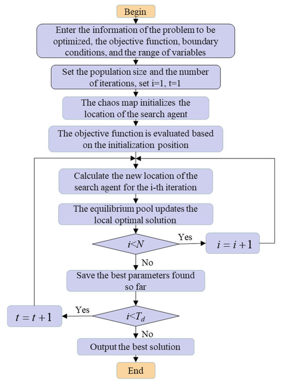
Figure 2. ISABO process framework.

2.3. ISABO-VMD-Based Signal Denoising Method

To address the uncertain decomposition level and penalty factor in the variational mode decomposition (VMD) process, this paper proposes a multi-strategy improved subtraction-average-based optimizer (ISABO) for adaptive parameter optimization. Through iterative computation of this enhanced optimization algorithm, optimal parameters are determined, thereby establishing a solid foundation for decomposing vibration signals from pumped storage units.

The proposed adaptive VMD method involves the following specific steps, with its workflow illustrated in Figure 3.

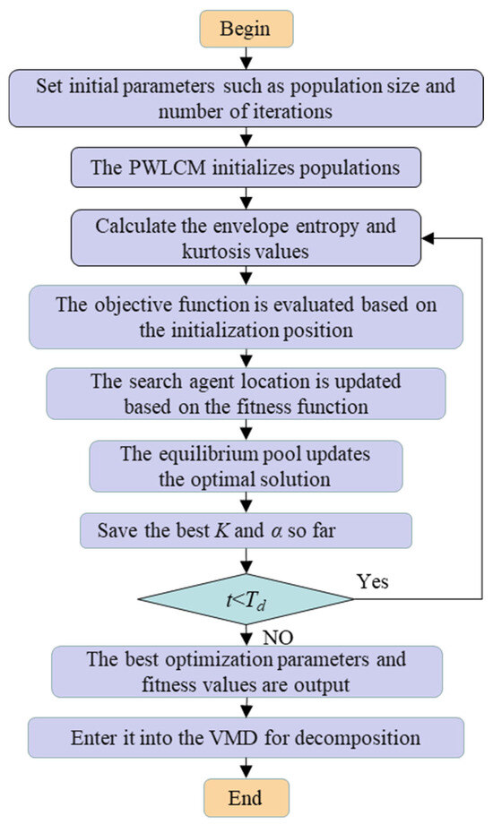
Figure 3. Flowchart of the improved VMD algorithm.

(1)

Initialize ISABO parameters;

(2)

Replace original random initialization with a PWLCM;

(3)

Calculate envelope entropy and kurtosis values followed by harmonic normalization processing;

(4)

Evaluate objective function based on initialized positions;

(5)

Update search agent positions according to the fitness function;

(6)

Update optimal solution via equilibrium pool mechanism;

(7)

Store currently found optimal A and B parameters;

(8)

Output optimal parameters and fitness value if maximum iterations are reached; otherwise, return to step (3).

2.4. Bidirectional Long Short-Term Memory (BILSTM) Network

The BILSTM model is an improved version of the standard LSTM framework, designed to enhance the understanding of temporal data by incorporating bidirectional processing along the time dimension. This architecture significantly improves the recognition of long-range dependencies by simultaneously capturing both forward and backward temporal patterns in sequential data. In the BILSTM structure, input data is first fed into the bidirectional network, where two sets of parameters work in concert to precisely regulate information flow to the hidden states, ultimately enabling effective feature classification through a softmax layer. The network architecture of the BILSTM is illustrated in Figure 4. The theoretical formulation is as follows:

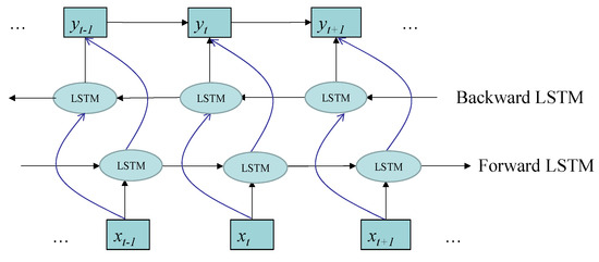
Figure 4. BILSTM network design.

The forward propagation computation process of the BILSTM network is formulated as follows in Equations (13) and (14):

$$h_t^{\left(1\right)}=f\left(U^{\left(1\right)}{h}_{t-1}^{\left(1\right)}+W^{\left(1\right)}{x}_t+b^{\left(1\right)}\right)$$

(13)

$$h_t^{\left(2\right)}=f\left(U^{\left(2\right)}{h}_{t+1}^{\left(2\right)}+W^{\left(2\right)}{x}_t+b^{\left(2\right)}\right)$$

(14)

The final hidden layer output constitutes the concatenation of opposing neuronal outputs from the preceding two layers.

$$y_t=g\left(U\left[h_t^{\left(1\right)};h_t^{\left(2\right)}\right]+c\right)$$

(15)

The softmax function is widely employed for classifying feature data in both supervised learning and deep learning. During the training process, it transforms the raw output scores of the network into probabilistic form and subsequently enhances the model’s classification accuracy by minimizing the loss function to better discriminate among different categories. Ultimately, the softmax classifier assigns the category with the highest probability as the predicted class.

$$f_y={\displaystyle {\sum }_{i=1}^d{W}_{yi}{x}_i=}{W}_{y}x$$

(16)

Here, $f_y$ and $W_{yi}$ represent the output and weights of the fully connected layer, respectively. The softmax method first maps each class output to $\left(0,+\infty \right)$ via an exponential function, followed by normalization for computation. The probability calculation for classification is given by Equation (17).

$$\mathrm{Softmax}\left(f_y\right)={\displaystyle \frac{e^{f_y}}{{\displaystyle {\sum }_{c=1}^C{e}^{f_c}}}}$$

(17)

The BILSTM deep neural network architecture comprises five core components: the input layer, the BILSTM layer, the fully connected layer, the softmax layer, and the output layer.

The BILSTM layer is configured with G hidden units. This layer employs the tanh function as the state activation function to capture long-term dependencies in sequential data while utilizing the sigmoid function as the gating activation function to regulate information flow and forgetting. The input layer is responsible for receiving raw data, whereas the BILSTM layer processes the input by incorporating both forward and backward contextual information, thereby generating feature representations enriched with contextual understanding. The fully connected layer takes the output of the BILSTM layer as its input vector, integrates and transforms the features, and subsequently, the softmax layer operates on the output of the fully connected layer to predict fault categories by computing probability distributions. A schematic illustration of fault classification using the softmax function is presented in Figure 5. Finally, the output layer displays the fault probability distribution computed by the softmax layer for subsequent decision-making or analysis, with the specific formulation given in Equation (18).

$$\begin{array}{l}tanh\left(x\right)={\displaystyle \frac{e^x-e^{-x}}{e^x+e^{-x}}}\\ sigmoid\left(x\right)={\displaystyle \frac{1}{1+e^{-x}}}\\ softmax\left(x_i\right)={\displaystyle \frac{e^{x_i}}{{\displaystyle {\sum }_{c=1}^C{e}^{x_c}}}}\end{array}$$

(18)

where $x$ denotes the input to the activation function, $x_i$ represents the i-th element in the input, and C indicates the number of fault categories.

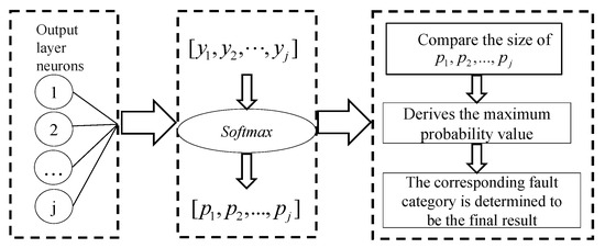
Figure 5. Schematic diagram of the fault classification of the softmax function.

2.5. ISABO-BILSTM Classification Model

The BILSTM model contains numerous manually configured hyperparameters. Specifically, the number of output layer units equals the dimensionality of the input data, and the number of fully connected units matches the output dimension. However, other parameters remain undetermined. Among these, three critical parameters—the number of hidden layer units, maximum training epochs, and learning rate—significantly impact the diagnostic model’s accuracy. By optimizing these three parameters using the ISABO algorithm (improved subtraction-average-based optimizer), we can avoid tedious trial-and-error processes and consequently enhance fault recognition accuracy. The parameter optimization process of the model is illustrated in Figure 6. The optimization procedure is as follows:

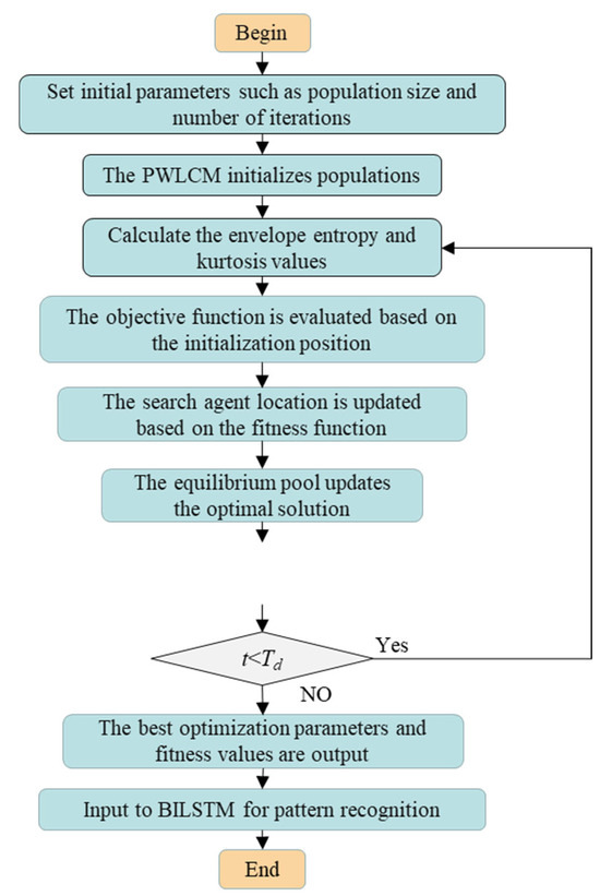
Figure 6. ISABO-BILSTM model parameter optimization process.

(1)

Initialize ISABO parameters: The fitness function for optimization combines envelope entropy and kurtosis into a composite evaluation metric.

(2)

Apply a PWLCM: Replaces the original random initialization process.

(3)

Calculate and normalize features: Compute both envelope entropy and kurtosis values, followed by harmonic normalization.

(4)

Evaluate objective function: Assessment based on initialized parameter positions.

(5)

Update search agents: Modify positions according to the fitness function results.

(6)

Optimize solution pool: Update the equilibrium pool with the current best solutions.

(7)

Store optimal parameters: Record the best-found values for the number of hidden layer units, the maximum training epochs, and the learning rate.

(8)

Termination check: If maximum iterations are reached, output optimal parameters and fitness value; otherwise, return to step (3).

3. Adaptive VMD-BILSTM-Based Fault Diagnosis Model for Pumped Storage Units

The proposed model employs the ISABO-optimized VMD and BILSTM parameters to achieve fault identification in pumped storage units. The overall workflow of the model is illustrated in Figure 7. The complete implementation procedure consists of the following steps:

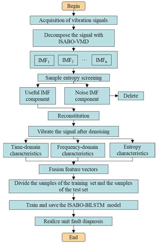
Figure 7. Flowchart of the fault diagnosis model of a pumped storage unit.

(1)

Acquisition of vibration data from pumped storage units;

(2)

Decomposition of initial signals using the adaptive VMD data processing model;

(3)

Calculation of sample entropy for each frequency component, with IMF components meeting composite threshold conditions being selected (optimal components are directly utilized while others are discarded as noise), followed by reconstruction of the denoised signal from the selected IMF components;

(4)

Computation of feature vector indicators from the denoised signal to construct the feature dataset. This study extracts a total of 26 feature vectors from vibration signals, comprising 2 entropy indicators, 14 time-domain indicators, and 10 frequency-domain indicators, to construct the feature dataset.

(5)

Division of feature vectors into training and testing sets according to a specified ratio;

(6)

Optimization of BILSTM parameters, including the number of hidden layer units (K), maximum training epochs (T), and learning rate (L);

(7)

Model training and subsequent fault identification for pumped storage units.

4. Case Study Analysis

4.1. Data Source

A case analysis was conducted using unit vibration and swing data collected from the condition monitoring system of a pumped storage power station, with the relevant parameters of the power station shown in Table 2. The collected unit vibration data underwent sliding window processing with a window spacing of 1000 and a sample length of 2048. The dataset comprises 480 samples covering four operational states, with 120 samples per state.

Table 2. Pumped storage power station unit parameters.

Name of the Parameter	Numeric Value of the Parameter
Generator output	268 MW
Factor	Pump condition: 0.98, turbine condition: 0.9;
Rated speed	333.3 r/min
Maximum rpm speed	535.0 r/min
Fixed number of guide vanes	20
Number of active guide vanes	20
Rotation frequency	50/9 Hz
Number of runner blades	9

Tsinghua University developed a DP-type low-frequency vibration sensor for vibration monitoring. The sensor’s most important feature is its lower frequency, 0.2~0.5 Hz, which is suitable for monitoring the vibrations of large- and medium-sized units. This sensor is used to measure the upper frame, the lower frame, the top cover, and the degree of large shaft swing of the pendulum. The system also includes the German Schenker company’s IN-081 integrated eddy current sensors and Switzerland’s KELLER company’s 21R series of pressure sensors, which have a high-frequency response and are suitable for pressure pulsation measurements. Figure 8 shows the layout for some of these sensors.

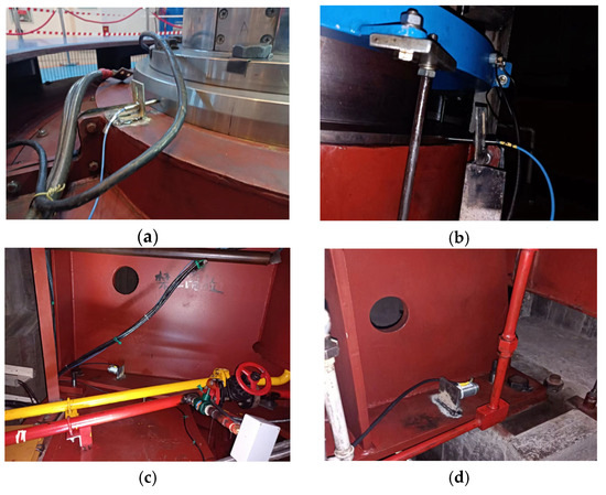
Figure 8. Sensor mounting position: (a) upper guided pendulum degree + Y; (b) lower guided pendulum degree + Y; (c) upper frame vibration + Y; and (d) lower frame vibration + Y.

The four operational states include normal condition signals, thrust head loosening signals, rotor-stator rubbing signals, and rotor misalignment signals. Figure 9 displays the time-domain waveforms of these four signal types, from which it can be observed that signals from different states exhibit distinct vibration amplitudes.

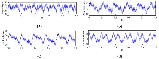
Figure 9. Time-domain diagram of different states of pumped storage units: (a) normal state; (b) loose thrust head; (c) rotor-stator rubbing; and (d) rotor misalignment.

4.2. ISABO-VMD-Based Raw Signal Denoising Process

The IASBO-VMD method was employed to separate the signals containing fault characteristics from the original signals. VMD optimization was conducted on four types of original signals corresponding to normal conditions, loose thrust collar, rotor-stator rubbing, and rotor misalignment, yielding the optimal parameter combinations tailored to each specific signal, which were (3, 1224), (5, 1536), (5, 1477), and (6, 5297), respectively. Subsequently, the vibration signal under the condition of rotor misalignment was taken as an example for analysis. The vibration characteristics caused by rotor misalignment are as follows: when the unit operates at no load and low rotational speed, significant vibration occurs, with the characteristic frequencies being the rotation frequency of the drive shaft and its higher harmonics, among which the second harmonic is the most prominent.

The vibration signal associated with rotor misalignment was decomposed using the ISABO-VMD method, and the results are illustrated in Figure 10. A total of six intrinsic mode function (IMF) components were extracted. Notably, there are significant spectral differences among these modes, with no overlapping of the central frequencies, indicating the absence of modal aliasing, over-decomposition, or under-decomposition phenomena. Based on the principles and characteristics of rotor misalignment faults, it can be preliminarily concluded that, after processing the original vibration signal with ISABO-VMD, the characteristic information of the fault has become apparent.

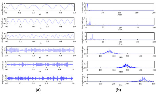
Figure 10. Misaligned rotor ISABO-VMD decomposition results: (a) decomposed time-domain plot and (b) decomposed spectrogram.

The sample entropy (SampEn) values of the six IMF components were calculated separately, and the corresponding bar chart is shown in Figure 11. A smaller SampEn value indicates higher self-similarity of the signal, whereas a larger SampEn value reflects greater signal complexity. As illustrated in Figure 11, the SampEn values of IMF1–3 components are relatively small and fall within the threshold range, indicating the highest self-similarity of the signal. Therefore, these components were selected for retention. The remaining IMF components were discarded as noise, and the denoised feature signal was reconstructed using IMF1–3, as shown in Figure 12. The results demonstrate that the reconstructed signal effectively reduces noise interference while preserving the primary characteristics of the original signal, thereby providing a more reliable data foundation for subsequent feature extraction and signal analysis. Comparative analysis reveals that the reconstruction algorithm achieves an optimal balance between noise suppression and feature retention, ensuring the integrity of the signal’s critical information.

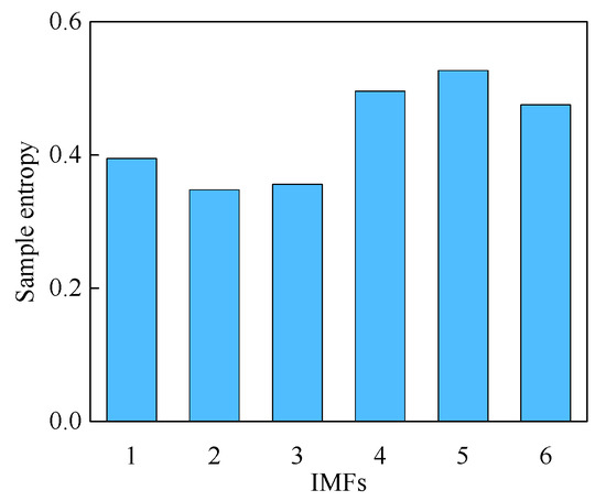
Figure 11. The calculated entropy of each IMF component sample.

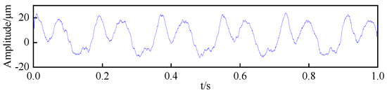
Figure 12. Final denoising results.

Feature extraction was performed on the denoised and reconstructed signals, where each fault type’s data was divided into 120 samples. For each sample, 26 time-frequency domain features were calculated, resulting in a feature matrix dataset of 480 rows × 26 columns. Focusing on two entropy indicators, the kurtosis factor from time-domain features and the central frequency from frequency-domain features, as key research parameters, the characteristic data scatter plot (Figure 13) demonstrates distinct feature distribution patterns among the four different fault categories. In the figure, green represents the Normal state, blue indicates Loose thrust head, red shows Rotor-stator rubbing, and purple denotes Rotor misalignment. This clear separability in feature space confirms the effectiveness of the processing method in extracting authentic vibration signal characteristics, thereby establishing a robust foundation for subsequent classification modeling.

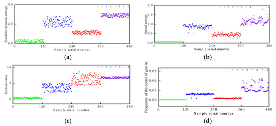
Figure 13. Four scatter plots of characteristic data: (a) symbolic dynamic entropy; (b) spread entropy; (c) kurtosis factor; and (d) frequency of the center of gravity.

4.3. Pattern Recognition and Comparative Analysis

During the optimization of BILSTM classifier parameters using the ISABO algorithm, the following configuration was adopted: optimization dimension D = 5; population size: 30; maximum iterations: 50. The optimization convergence curve (Figure 14) demonstrates that the process reached stability after 12 iterations, yielding the optimal parameters: number of hidden units (K): 39; maximum training epochs (T): 100; learning rate (L): 0.0526. The finalized hyperparameters after ISABO optimization are systematically presented in Table 3.

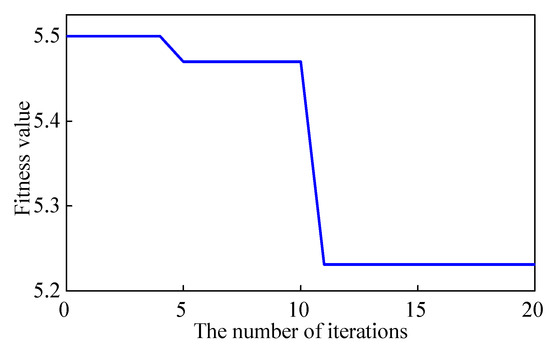
Figure 14. Iterative process of the ISABO fitness function.

Table 3. Optimal values of BILSTM hyperparameters.

Name of the Parameter	Optimal Value
Number of hidden layer elements K	39
Maximum training period T	100
Learning rate L	0.0562

To validate the effectiveness and superiority of the BILSTM model, this study compares several common pattern recognition models, including BP neural network, random forest, support vector machine, and extreme learning machine. Feature datasets are input into different models for training and classification, with each model being run 10 times to obtain the average accuracy. The results are shown in Figure 15 and Table 4. From Figure 15 and Table 4, it can be observed that under normal operating conditions, thrust head looseness, dynamic and static friction, and rotor misalignment conditions, the accuracy of diagnosis using the BILSTM model is significantly higher than that of other models. The accuracies of the BP, RF, SVM, and ELM models are 79.65%, 81.97%, 81.31%, and 83.67%, respectively, while the BILSTM model achieves an accuracy of 89.56%. This indicates that the diagnostic performance of the BILSTM model surpasses that of other similar models.

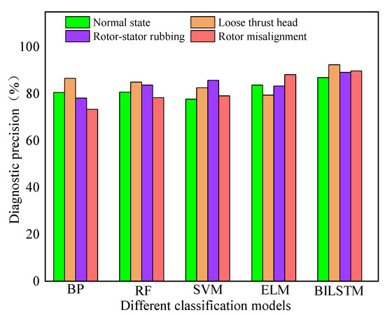
Figure 15. Comparison of different diagnostic models.

Table 4. Accuracy of different diagnostic models.

Type of Failure	Average Accuracy/%
	BP	RF	SVM	ELM	BILSTM
Normal State	80.52	80.77	77.75	83.77	86.95
Loose Thrust Head	86.56	84.96	82.58	79.43	92.39
Rotor-Stator Rubbing	78.14	83.78	85.75	83.34	89.18
Rotor Misalignment	73.38	78.39	79.14	88.14	89.75
Comprehensive Accuracy	79.65	81.97	81.31	83.67	89.56

To validate the effectiveness of the denoising method proposed in this paper, comparison experiments were set up. The denoised dataset and the undenoised dataset were input into the bidirectional long short-term memory network (BILSTM), respectively, with the number of BILSTM hidden layer units set to K = 39, the maximum training cycles set to T = 100, and the learning rate set to L = 0.0526. Feature extraction was not performed, and a sliding window method was used to expand each type of raw data into 120 samples, with 75% used for model training and the remaining 25% for testing the model’s accuracy. The diagnostic results in both cases are shown in Figure 16 and Figure 17.

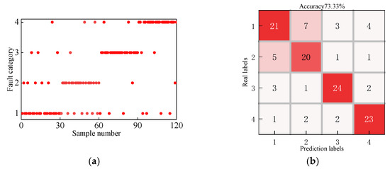
Figure 16. Classification result plot of the undenoised data: (a) scatter plot of the raw data classification results and (b) raw data classification confusion matrix.

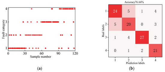
Figure 17. Classification result plot of the denoised processing data: (a) scatter plot of the denoised data classification results and (b) denoised data classification confusion matrix.

As can be seen from Figure 16, the data that has not undergone denoising treatment has a recognition accuracy of 73.33%. From the confusion matrix, the number of successful recognitions for the four labels is 21, 20, 24, and 23, respectively, with the erroneous recognitions being 9, 10, 6, and 7. The second category has the highest error rate at 33.33%, while the third category has the highest recognition accuracy at 80%. The overall combined recognition accuracy for the four categories is 73.33%.

From Figure 17, it can be seen that directly performing pattern recognition on the denoised signals improves classification accuracy compared to the original data. The number of correctly recognized samples among the four identification categories is 24, 20, 27, and 21, respectively, with erroneous recognitions being 6, 10, 3, and 9. The second category has the lowest recognition accuracy at 66.67%, while the third category has the highest recognition accuracy at 90%. The overall combined recognition rate is 76.66%, which is an increase of 3.33% compared to the 73.33% without denoising. This indicates that the denoising model proposed in this paper has a positive effect on improving the fault recognition accuracy of actual pumped storage unit vibration signals, and it lays a foundation for the subsequent feature extraction and pattern recognition.

In order to illustrate the superiority of the ISABO-optimized BILSTM diagnostic model, the ISABO-BILSTM diagnostic model proposed in this paper is compared with the optimized BILSTM diagnostic models of SABO, GWO, and PSO, respectively, and the basic parameters of different models are set to the same values. Table 5 shows the composite accuracy results of the different models.

Table 5. Accuracy of different diagnostic models.

Type of Failure	Average Accuracy/%
	PSO-BILSTM	GWO-BILSTM	SABO-BILSTM	ISABO-BILSTM
Normal State	88.65	85.07	86.42	96.29
Loose Thrust Head	89.41	94.18	94.71	98.60
Rotor-Stator Rubbing	92.68	93.70	95.63	97.34
Rotor Misalignment	93.86	87.98	91.12	99.59
Comprehensive Accuracy	91.15	90.23	91.97	97.96

As can be seen from Table 5, ISABO-BILSTM has the highest diagnostic accuracy, in which the loose thrust head accuracy is 98.60%, the dynamic and static friction is 97.34%, the rotor misalignment is 99.59%, the diagnostic accuracy for the four faults is higher than 96%, and the composite accuracy is 97.96%. The composite accuracy of the BILSTM diagnostic model optimized by PSO, GWO, and SABO was 91.15%, 90.23%, and 91.97%, respectively. Compared with the above three models, the accuracy of the ISABO-BILSTM diagnostic model proposed in this paper is increased by 6.81%, 7.73%, and 5.99%, respectively.

The test set included a total of 120 samples, with 109, 107, 110, and 117 samples correctly identified by PSO, GWO, SABO, and ISABO, respectively, and 11, 13, 10, and 3 incorrectly identified samples. It can be seen that the BILSTM model, after ISABO parameter optimization, shows stronger identification ability, and its ability to accurately identify fault samples is more convenient than that of expert experience to artificially determine model parameters. It can also shorten the labor time cost, which benefits the operation and maintenance personnel of pumped storage power stations. The case study results show that the proposed model has higher reliability.

The precision, recall, and F1 scores of different classification models are shown in Table 6, from which it can be seen that all the indexes of the ISABO-BILSTM classification model show good performance and are more adaptable for pumped storage unit fault diagnosis compared to other similar models.

Table 6. Indicators for evaluating the diagnostic results of different classification models.

Classification Model	Evaluation Indicators
	Precision/%	Recall/%	F1 Score/%
PSO-BILSTM	91.15	91.27	91.21
GWO-BILSTM	90.23	90.17	90.20
SABO-BILSTM	91.97	91.13	91.55
ISABO-BILSTM	97.96	97.06	97.51

In order to further validate the effectiveness of the model, during the fault identification process, BP, RF, SVM, ELM, and BILSTM were each trained 20 times using the same feature dataset, recording the accuracy of each model during the training process, and constructing a diagnostic accuracy curve, as shown in Figure 18. From the figure, it can be seen that the accuracy curve of BILSTM is comparatively higher than that of other models, with an accuracy range of [0.85, 0.95] and an overall accuracy of 89.56%. The distribution of the BP neural network is the lowest, with a classification accuracy range of [0.73, 0.86] and an overall accuracy of 79.65%, while the accuracy ranges of the other models fall between these two.

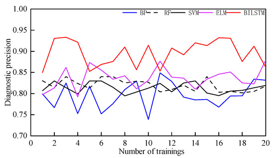
Figure 18. Comparison chart of the accuracy of traditional models across training sessions.

Similarly, the four classification models, PSO-BILSTM, GWO-BILSTM, SABO-BILSTM, and ISABO-BILSTM, were trained 20 times using the same feature dataset, and their multiple training comparison is shown in Figure 19. From the figure, it can be seen that compared to the BILSTM model without parameter optimization, the diagnostic accuracy of the models optimized by the four algorithms has significantly improved, with increases of 1.59%, 0.67%, 2.41%, and 8.4%, respectively, further demonstrating the superiority of the model proposed in this paper. The classification accuracy ranges for the four models are [0.88, 0.93], [0.85, 0.94], [0.86, 0.95], and [0.96, 0.99], with ISABO-BILSTM clearly in the lead. Its minimum value was higher than the minimum value of GWO-BILSTM by 0.11 and also higher by 0.1 compared to the unmodified SABO-BILSTM, indicating that the combined model proposed in this paper has certain advantages over other similar models while also verifying the improvement strategy for SABO discussed earlier.

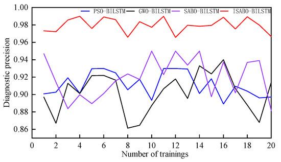
Figure 19. Comparison chart of the accuracy of different optimization models across training sessions.

5. Conclusions

This paper proposes a fault diagnosis method for units based on adaptive VMD and BILSTM. The model demonstrates good accuracy and practicality in identifying unit faults. The main conclusions of this paper are as follows:

(1)

Aiming at the non-stationary and nonlinear vibration signals generated by faults in pumped storage units, an adaptive parameter optimization method for variational mode decomposition (VMD) based on the improved subtraction-average-based optimizer (ISABO) is proposed. By combining the piecewise linear chaotic map (PWLCM) with the balanced pool embedding strategy, the method achieves adaptive optimization of the VMD penalty factor and the number of decomposition layers. Experimental results demonstrate that the proposed ISABO-VMD method can effectively realize the adaptive selection of parameters.

(2)

To address the significant impact of key hyperparameters, such as the number of hidden units in the BILSTM network, the maximum number of training epochs, and the learning rate on diagnostic accuracy, the ISABO algorithm is introduced into the parameter optimization process. By establishing a fitness function and constraint conditions, the three key parameters are optimized in a coordinated manner, resulting in the construction of the ISABO-BILSTM intelligent diagnostic model. The experimental results indicate that, compared with traditional parameter-setting methods, the ISABO-BILSTM model demonstrates significant performance advantages, with an overall diagnostic accuracy rate reaching 97.96%.

The VMD-BILSTM fault diagnosis model optimized by the ISABO proposed in this paper has achieved remarkable results in both theoretical research and experimental verification, providing a new idea with practical significance for the fault diagnosis of pumped storage units. However, there are still a number of urgent problems to be solved in practical engineering applications, which are mainly reflected in the following aspects that need in-depth research and improvement: (1) The diagnostic model proposed in the paper should select parameters and data according to local conditions in practice, and complete data samples are an important factor for the diagnostic model to be successful. Therefore, it is necessary to further expand the fault data samples in order to achieve a higher accuracy rate. (2) In this paper, single faults of different fault types of pumped storage units under specific rotational frequencies are investigated; however, coupled faults of multiple faults may occur in the units in actual working conditions. Therefore, further exploration of fault diagnostic models that can adapt to compound faults with variable rotational speeds is needed.

References

- Chin, C.H.; Abdullah, S.; Ariffin, A.K.; Singh, S.S.K.; Arifin, A. A review of the wavelet transform for durability and structural health monitoring in automotive applications. Alex. Eng. J. 2024, 99, 204–216. [Google Scholar] [CrossRef]
- Lv, Y.; Wang, J.; Zhang, C.; Ding, J. Composite fault feature extraction for gears based on MCKD-EWT adaptive wavelet threshold noise reduction. Meas. Control 2025, 58, 185–195. [Google Scholar] [CrossRef]
- Yu, K.; Feng, L.; Chen, Y.; Wu, M.; Zhang, Y.; Zhu, P.; Chen, W.; Wu, Q.; Hao, J. Accurate wavelet thresholding method for ECG signals. Comput. Biol. Med. 2024, 169, 107835. [Google Scholar] [CrossRef]
- Long, S.H.; Zhou, G.Q.; Wang, H.Y. Denoising of lidar echo signal based on wavelt adaptive threshold method. Adv. Civ. Eng. 2020, 3, 215–220. [Google Scholar]
- Huang, H.R.; Li, K.; Su, W.S. An improved empirical wavelet transform method for rolling bearing fault diagnosis. Sci. China Technol. Sci. 2020, 63, 2231–2240. [Google Scholar] [CrossRef]
- Dong, J.; Zhang, Y.; Hu, J. Short-term air quality prediction based on EMD-transformer-BiLSTM. Sci. Rep. 2024, 14, 20513. [Google Scholar] [CrossRef]
- Xu, D.; Yin, J. An enhanced hybrid scheme for ship roll prediction using support vector regression and TVF-EMD. Ocean. Eng. 2024, 307, 117951. [Google Scholar] [CrossRef]
- Karbasi, M.; Ali, M.; Farooque, A.A.; Jamei, M.; Khosravi, K.; Cheema, S.J.; Yaseen, Z.M. Robust drought forecasting in Eastern Canada: Leveraging EMD-TVF and ensemble deep RVFL for SPEI index forecasting. Expert Syst. Appl. 2024, 256, 124900. [Google Scholar] [CrossRef]
- Liu, C.C.; Yang, Z.; Shi, Q. A gyroscope signal denoising method based on empirical mode decomposition and signal reconstruction. Sensors 2019, 19, 5064. [Google Scholar] [CrossRef]
- Cai, J.H.; Hu, W.W.; Wang, X.C. Fault Diagnosis ofRolling Bearing Based on EMD-ICA De-noising. J. Mach. Des. 2015, 32, 17. [Google Scholar]
- Dragomiretskiy, K.; Zosso, D. Variational mode decomposition. IEEE Trans. Signal Process. 2014, 62, 531–544. [Google Scholar] [CrossRef]
- Li, Z.; Chen, J.; Zi, Y.; Pan, J. Independence-oriented VMD to identify fault feature for wheel set bearing fault diagnosis of high speed locomotive. Mech. Syst. Signal Process. 2017, 85, 512–529. [Google Scholar] [CrossRef]
- Cui, S.; Lyu, S.; Ma, Y.; Wang, K. Improved informer PV power short-term prediction model based on weather typing and AHA-VMD-MPE. Energy 2024, 307, 132766. [Google Scholar] [CrossRef]
- Qin, C.; Huang, G.; Yu, H.; Zhang, Z.; Tao, J.; Liu, C. Adaptive VMD and multi-stage stabilized transformer-based long-distance forecasting for multiple shield machine tunneling parameters. Autom. Constr. 2024, 165, 105563. [Google Scholar] [CrossRef]
- Ding, M.; Du, B.; Wan, H.; Han, L. A signal de-noising method for a MEMS gyroscope based on improved VMD-WTD. Meas. Sci. Technol. 2021, 32, 095112. [Google Scholar] [CrossRef]
- Mao, M.; Zhou, C.; Xu, B.; Liao, D.; Yang, J.; Liu, S.; Li, Y.; Tang, T. Fault diagnosis method using MVMD signal reconstruction and MMDE-GNDO feature extraction and MPA-SVM. Front. Phys. 2024, 12, 1301035. [Google Scholar] [CrossRef]
- Huang, Y.; Lin, J.; Liu, Z. A modified scale-space guiding variational mode decomposition for high-speed railway bearing fault diagnosis. J. Sound Vib. 2019, 444, 216–234. [Google Scholar] [CrossRef]
- Zhao, Y.J.; Li, C.S.; Fu, W.L. A modified variational mode decomposition method based on envelope nesting and multi-criteria evaluation. J. Sound Vib. 2019, 468, 115099. [Google Scholar] [CrossRef]
- Jiang, W.; Zhou, J.Z.; Liu, H. A multi-step progressive fault diagnosis method for rolling element bearing based on energy entropy theory and hybrid ensemble auto-encoder. ISA Trans. 2019, 87, 235–250. [Google Scholar] [CrossRef]
- Maulik, S.; Konar, P.; Chattopadhyay, P. Fusion of vibration and current signals for improved multi class fault diagnosis of three phase induction motor. In Proceedings of the 2023 IEEE 3rd Applied Signal Processing Conference (ASPCON), Haldia, India, 24–25 November 2023; pp. 152–155. [Google Scholar]
- Cao, H.; Shao, H.; Liu, B.; Cai, B.; Cheng, J. Clustering-guided novel unsupervised domain adversarial network for partial transfer fault diagnosis of rotating machinery. IEEE Sens. J. 2022, 22, 14387–14396. [Google Scholar] [CrossRef]
- Hong, G.; Suh, D. Mel Spectrogram-based advanced deep temporal clustering model with unsupervised data for fault diagnosis. Expert Syst. Appl. 2023, 217, 119551. [Google Scholar] [CrossRef]
- Wan, L.; Zhang, G.; Li, H.; Li, C. A novel bearing fault diagnosis method using spark-based parallel ACO-K-means clustering algorithm. IEEE Access 2021, 9, 28753–28768. [Google Scholar] [CrossRef]
- Rahimilarki, R.; Gao, Z.; Jin, N.; Zhang, A. Convolutional neural network fault classification based on time-series analysis for benchmark wind turbine machine. Renew. Energy 2022, 185, 916–931. [Google Scholar] [CrossRef]
- Chen, X.; Zhang, B.; Gao, D. Bearing fault diagnosis base on multi-scale CNN and LSTM model. J. Intell. Manuf. 2021, 32, 971–987. [Google Scholar] [CrossRef]
- Shi, X.; Qiu, G.; Yin, C.; Huang, X.; Chen, K.; Cheng, Y.; Zhong, S. An improved bearing fault diagnosis scheme based on hierarchical fuzzy entropy and Alexnet network. IEEE Access 2021, 9, 61710–61720. [Google Scholar] [CrossRef]
- Zou, F.; Zhang, H.; Sang, S.; Li, X.; He, W.; Liu, X. Bearing fault diagnosis based on combined multiscale weighted entropy morphological filtering and bi-LSTM. Appl. Intell. 2021, 51, 6647–6664. [Google Scholar] [CrossRef]
- Liu, Z.; Peng, Z.; Liu, P. Multi-feature optimized VMD and fusion index for bearing fault diagnosis method. J. Mech. Sci. Technol. 2023, 37, 2807–2820. [Google Scholar] [CrossRef]
- Trojovský, P.; Dehghani, M. Subtraction-average-based optimizer: A new swarm-inspired metaheuristic algorithm for solving optimization problems. Biomimetics 2023, 8, 149. [Google Scholar] [CrossRef]
Disclaimer/Publisher’s Note: The statements, opinions and data contained in all publications are solely those of the individual author(s) and contributor(s) and not of MDPI and/or the editor(s). MDPI and/or the editor(s) disclaim responsibility for any injury to people or property resulting from any ideas, methods, instructions or products referred to in the content. |
© 2025 by the authors. Licensee MDPI, Basel, Switzerland. This article is an open access article distributed under the terms and conditions of the Creative Commons Attribution (CC BY) license (https://creativecommons.org/licenses/by/4.0/).