
Improved Weighted Chimp Optimization Algorithm Based on Fitness–Distance Balance for Multilevel Thresholding Image Segmentation


Abstract
1. Introduction
- Methodological Innovation: This research presents the first application of the Weighted Chimp Optimization Algorithm (WChOA) to multilevel image segmentation, enhanced through integration with the Fitness–Distance Balance (FDB) method to develop WChOA-FDB, a novel hybrid metaheuristic optimization approach.
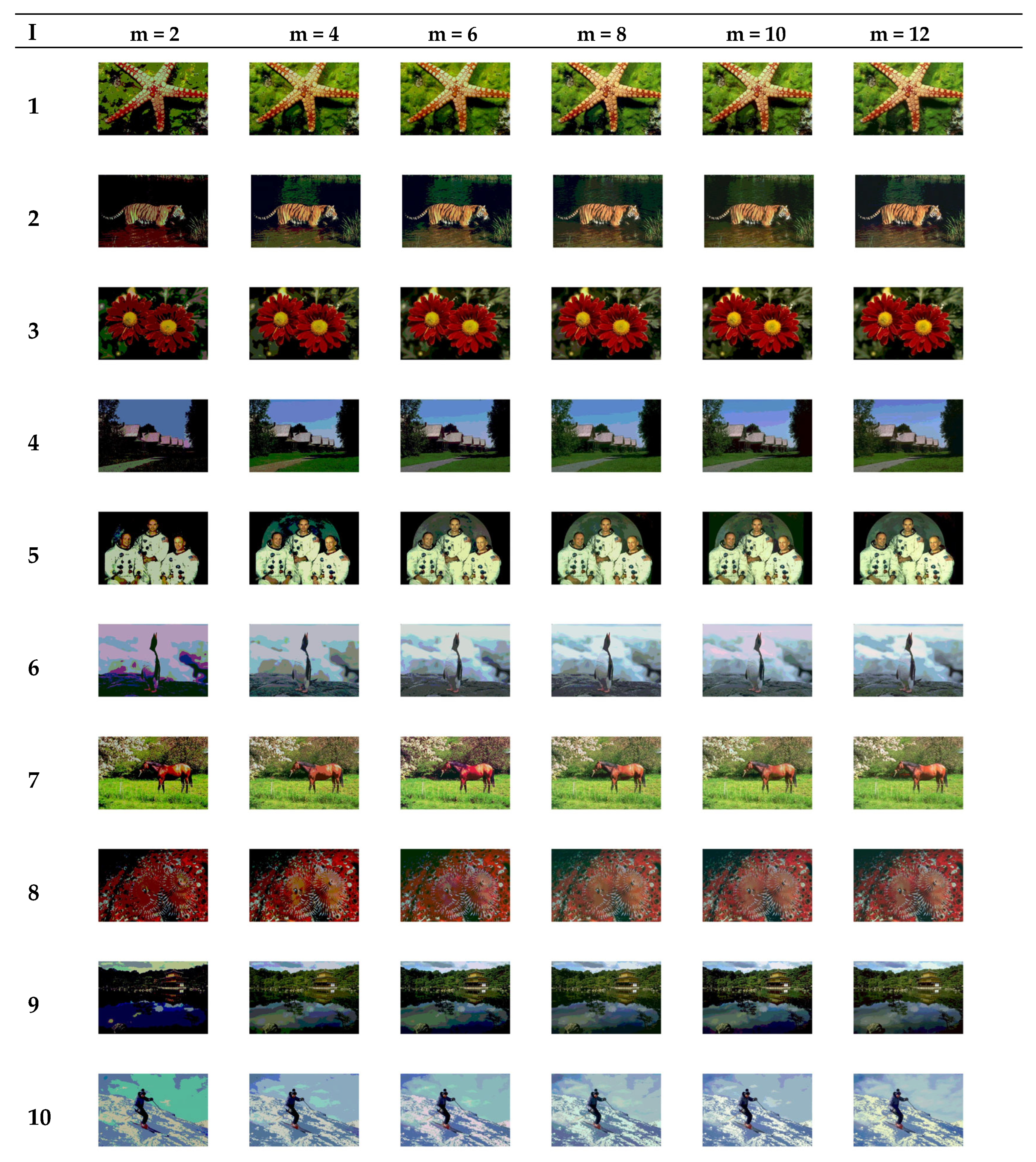
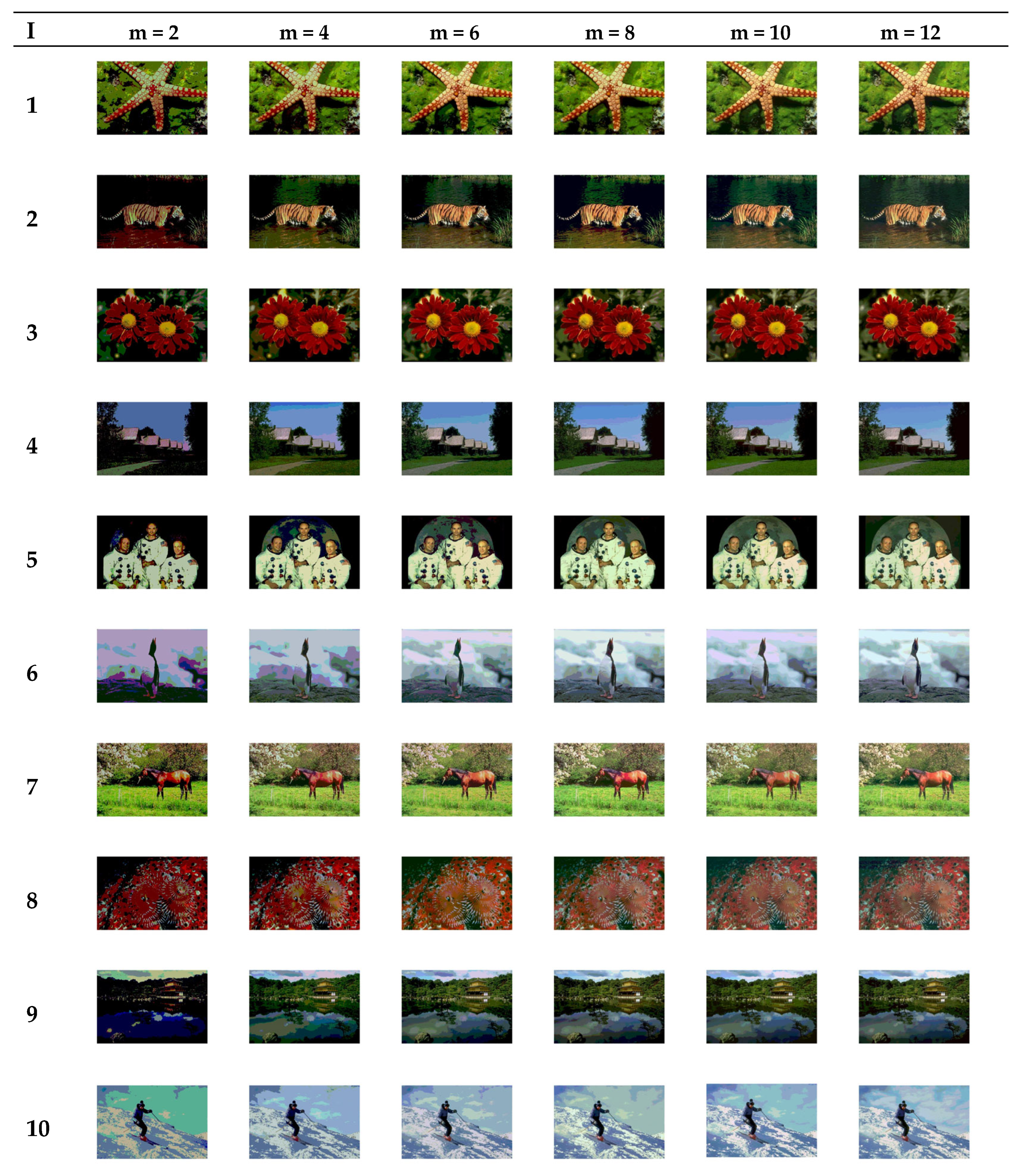
- Comprehensive Experimental Framework: The proposed WChOA-FDB algorithm was systematically evaluated through rigorous experimentation encompassing ten IEEE CEC 2020 benchmark functions of varying complexity, multilevel segmentation scenarios ranging from low to high threshold levels (m = 2, 4, 6, 8, 10, 12), comparative analysis against seven established metaheuristic algorithms, and assessment under different computational constraints (500 × m and 1000 × m maximum function evaluations).
- Empirical Validation and Performance Assessment: The efficacy of the proposed approach was thoroughly validated through multi-dimensional evaluation criteria, incorporating both optimization performance metrics (fitness function values) and established image quality assessment measures (Peak Signal-to-Noise Ratio (PSNR), Structural Similarity Index (SSIM), and Feature Similarity Index (FSIM)), demonstrating superior performance across diverse segmentation complexity levels.
2. Related Work
3. Materials and Methods
3.1. Multilevel Thresholding Problem
3.1.1. Kapur’s Entropy-Based Thresholding
3.1.2. Between-Class Variance-Based Thresholding (Otsu’s Method)
3.2. Proposed Method
3.2.1. WChOA Algorithm
3.2.2. Fitness–Distance Balance Selection
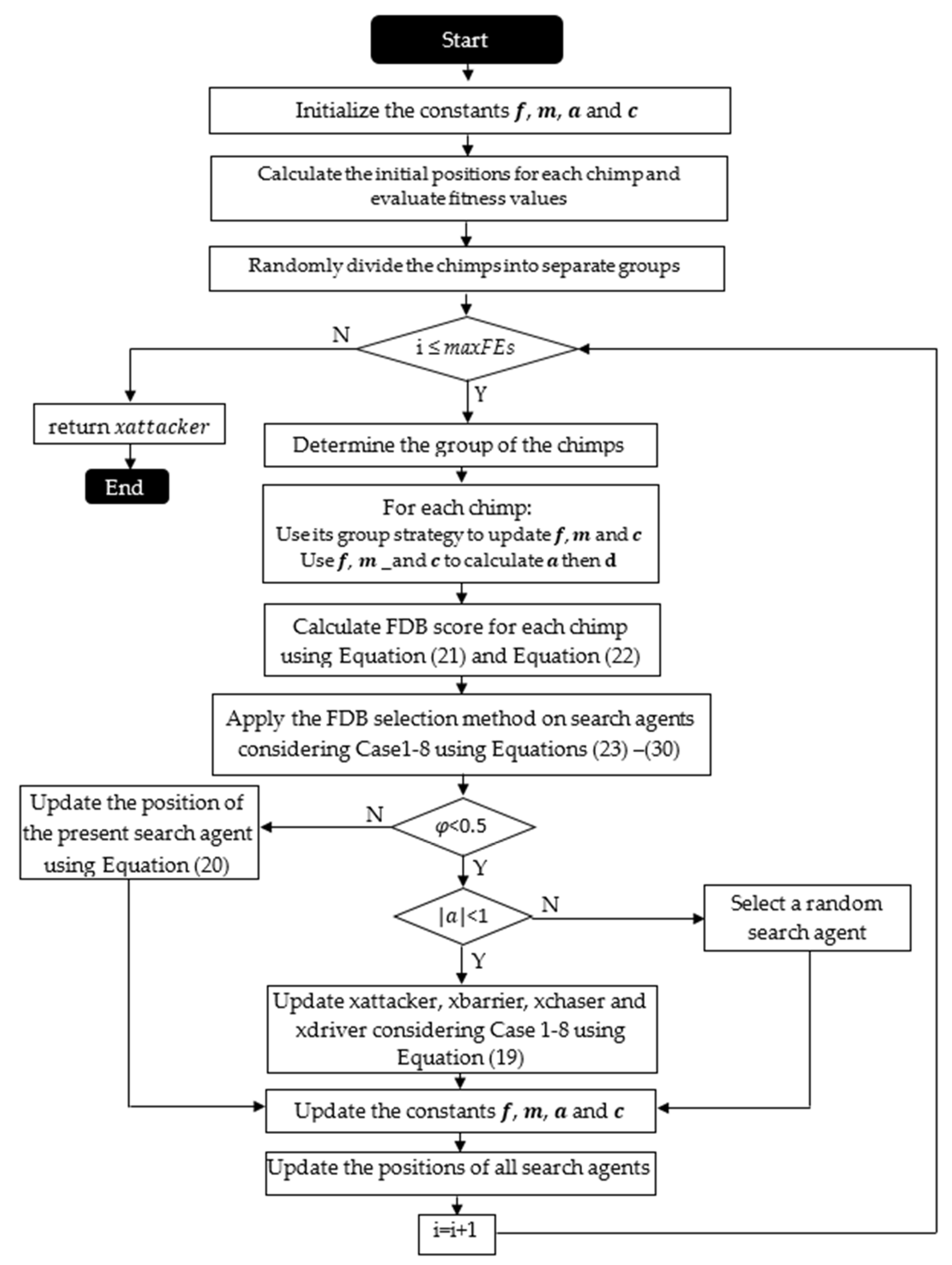
3.2.3. Proposed WChOA-FDB Scheme
- Initialization with FDB Parameters: WChOA-FDB begins by initializing a population of potential solutions, incorporating parameters specific to FDB.
- Evaluation and Fitness Assignment: Each solution is evaluated based on the objective function, and the fitness is assigned. FDB principles contribute to fitness assessment by considering the distances between solutions.
- Weighted Solution Evaluation with FDB: The weighted evaluation mechanism, enriched by FDB, assigns weights to solutions based on both their fitness and distances. This weighted approach guides subsequent decision-making processes.
- Collaborative Decision-Making Enhanced by FDB: Solutions engage in collaborative decision-making, now with added guidance from FDB. The algorithm prioritizes solutions not only based on their fitness but also considering their contribution to maintaining diversity within the population.
- Dynamic Adaptation with FDB: WChOA-FDB dynamically adapts its parameters throughout the optimization process, influenced by FDB. This ensures a continuous and adaptive exploration–exploitation balance.
- Iterative Optimization Enhanced by FDB: The algorithm iteratively optimizes solutions, leveraging the integrated FDB principles to achieve a balance between exploration and exploitation. Iterations continue until the termination criterion is met.
- Termination and Solution Retrieval: WChOA-FDB concludes when the termination criterion is satisfied. The best solutions, considering both fitness and distances, are retrieved as the final optimized outcomes.
| Algorithm 1. Pseudo-code of proposed WChOA-FDB algorithm |
| 1. Input: Chimp population (p), Number of iteration (Max_iter), |
| Problem dimension (number of variables) (d) |
| 2. Output: X_Attacker |
| 3. Begin: |
| 4. Initialize the constants f, m, a and c |
| 5. Calculate the initial position (population) for each chimp and evaluate fitness |
| 6. Randomly divide the chimps into separate groups |
| 7. for i = 1:p do |
| 8. Evaluate the fitness of each chimp |
| 9. end for |
| 10. xattacker = the best search agent |
| 11. xbarrier = the second best search agent |
| 12. xchaser = the third best search agent |
| 13. xdriver = the fourth best search agent |
| 14. //Meta-heuristic search process// |
| 15. while (l < Max_iter) //Number of iteration is not achieved |
| 16. for i = 1: p do |
| 17. for each chimp: |
| 18. Extract the chimp’s group |
| 19. Use its group strategy to update f, m and c |
| 20. Use f, m _and c to calculate a then d |
| 21. end for |
| 22. //Implementation of FDB selection method// |
| 23. for i = 1:p do |
| 24. Calculate Euclidean distance for each chimp using Equation (21) |
| 25. Calculate FDB score for each chimp using Equation (22) |
| 26. end for |
| 27. Create D and S as vectors using Equation (21) and Equation (22), respectively |
| 28. Determine x_FDB based on FDB philosophy by using Equation (9) |
| 29. Calculate d_Driver using Equation (23)//Case-1// |
| 30. Calculate d_Driver using Equation (24)//Case-2// |
| 31. Calculate d_Attacker and d_Driver using Equation (25)//Case-3// |
| 32. Calculate d_Attacker and d_Driver using Equation (26)//Case-4// |
| 33. Calculate d_Attacker and d_Driver using Equation (27)//Case-5// |
| 34. Calculate d_Attacker and d_Driver using Equation (28)//Case-6// |
| 35. Calculate d_Barrier and d_Driver using Equation (29)//Case-7// |
| 36. Calculate d_Barrier and d_Driver using Equation (30)//Case-8// |
| 37. Calculate d_Chaser using Equation (9) |
| 38. end for |
| 39. for i = 1: p do |
| 40. if (φ < 0.5) |
| 41. if (|a| < 1) |
| 42. Update the position of the driver by Equation (19)//Case-1// |
| 43. Update the position of the driver by Equation (19)//Case-2// |
| 44. Update the position of the attacker and driver by Equation (19)//Case-3// |
| 45. Update the position of the attacker and driver by Equation (19)//Case-4// |
| 46. Update the position of the attacker and driver by Equation (19)//Case-5// |
| 47. Update the position of the attacker and driver by Equation (19)//Case-6// |
| 48. Update the position of the barrier and driver by Equation (19)//Case-7// |
| 49. Update the position of the barrier and driver by Equation (19)//Case-8// |
| 50. Update the position of the chaser by Equation (19) |
| 51. else if (|a| > 1) |
| 52. Select a random search agent |
| 53. end if |
| 54. else if (φ > 0.5) |
| 55. Update the position of the present search agent by Equation (20) |
| 56. end if |
| 57. end for |
| 58. Update the constants f, m, a and c |
| 59. Update xattacker, xbarrier, xchaser and xdriver |
| 60. end while |
| 61. return xattacker |
4. Experimental Results
4.1. Experimental Settings
- The IEEE CEC 2020 suite [48], which has four different types of benchmark problems, was used to investigate the performance of the proposed algorithm.
- The optimization process termination criterion is determined by the maximum number of objective function evaluations, denoted as maxFEs. This criterion is set as maxFEs = 1000 × D, where D represents the problem dimension.
- The experiments were conducted independently for four varying problem dimensions (D = 10, D = 30, D = 50, and D = 100) to analyze and evaluate the performance of the proposed algorithm in low, medium, and high-dimensional optimization scenarios.
- The experiments were repeated 25 times for the optimization of each problem.
- Statistical test methods were employed to analyze the data obtained from experimental studies.
- Pairwise comparisons were conducted using the Wilcoxon test, while multiple comparisons were performed using the Friedman test.
- Experiments were conducted utilizing MATLAB R2018b on a Core i7 1065G7 1.30 GHz CPU with 12 GB of RAM and running Windows 11.
4.2. Testing and Analyzing the Performance of the Proposed WChOA-FDB Algorithm
Statistical Analyses on CEC’2020 Test Suite
4.3. Image Segmentation Performance of the Proposed WChOA-FDB Method
4.3.1. Statistical Analysis on Test Images
4.3.2. Performance Metrics
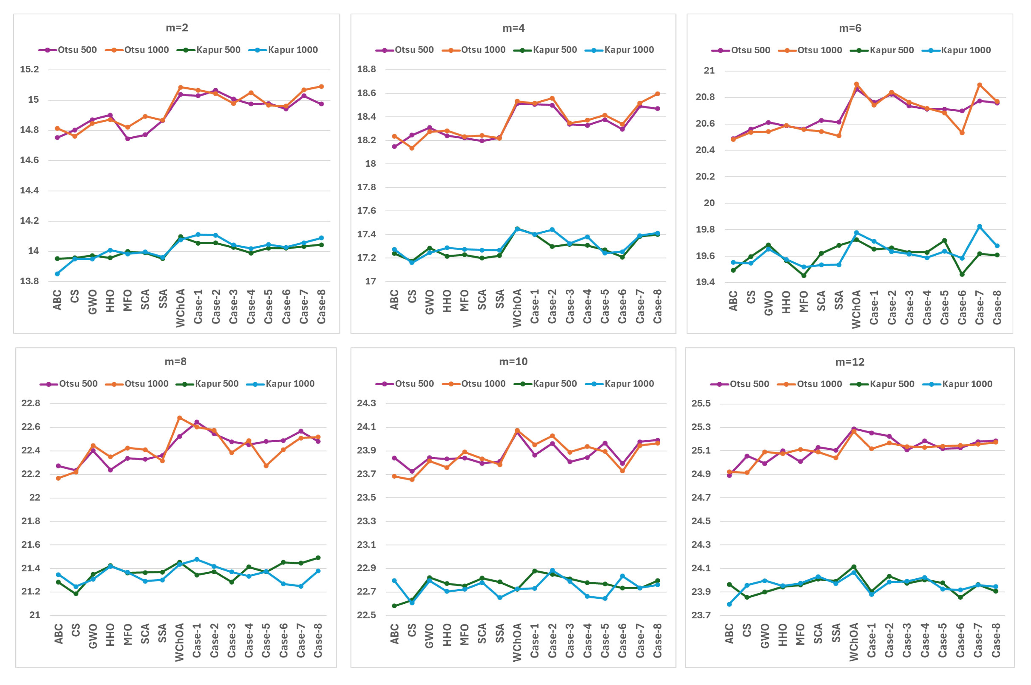
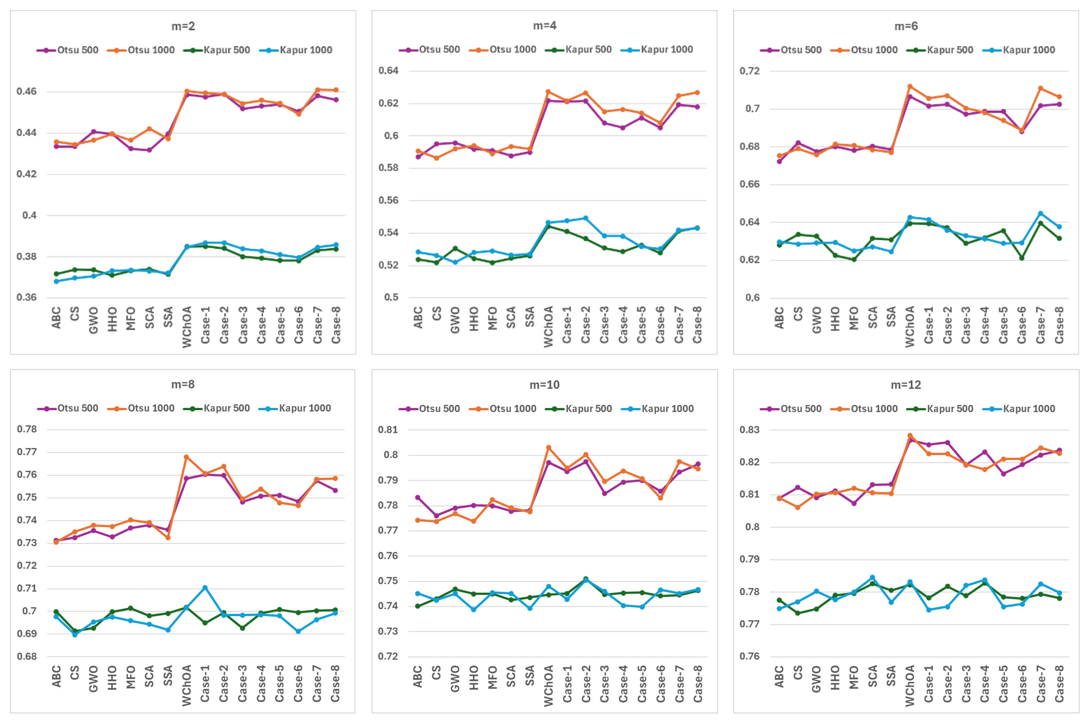
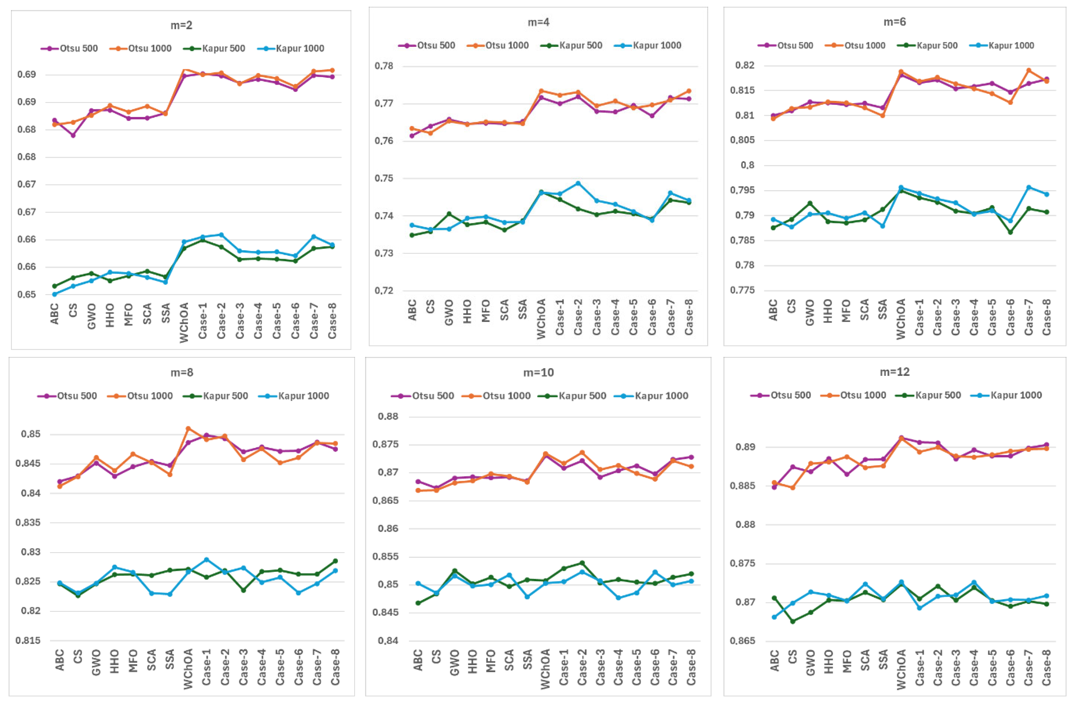
4.3.3. Performance Evaluation Using the Fitness Function
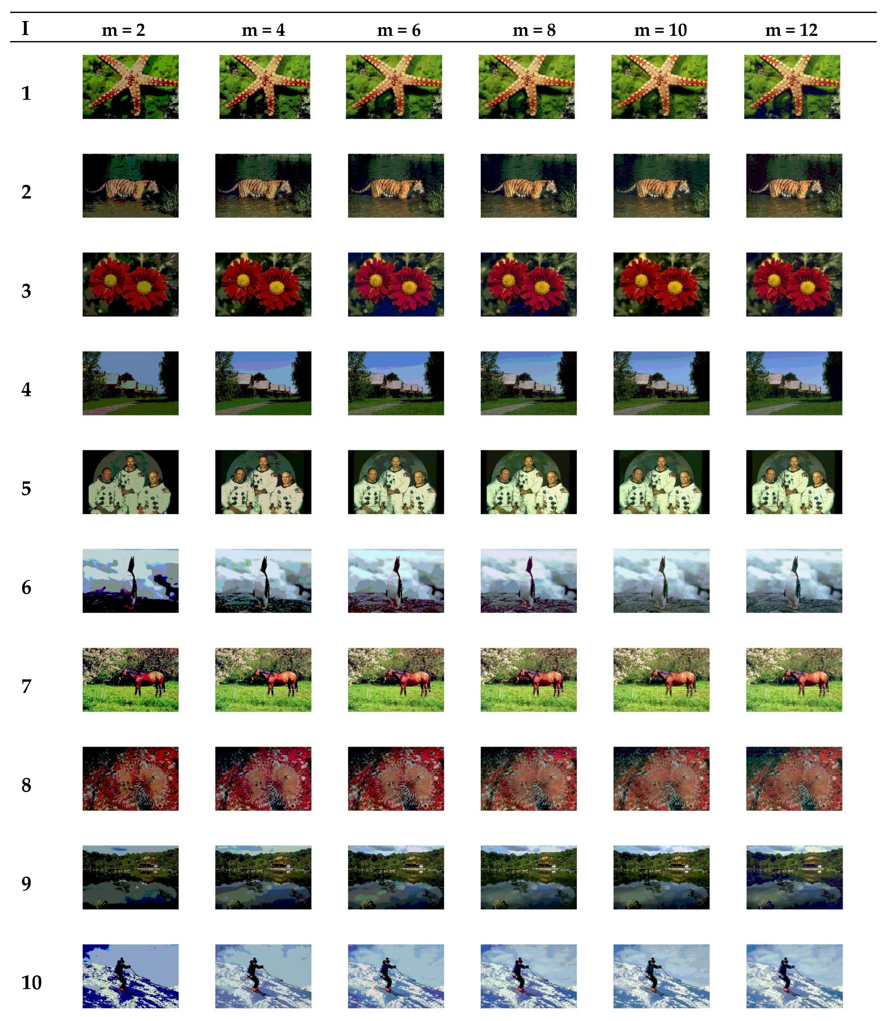
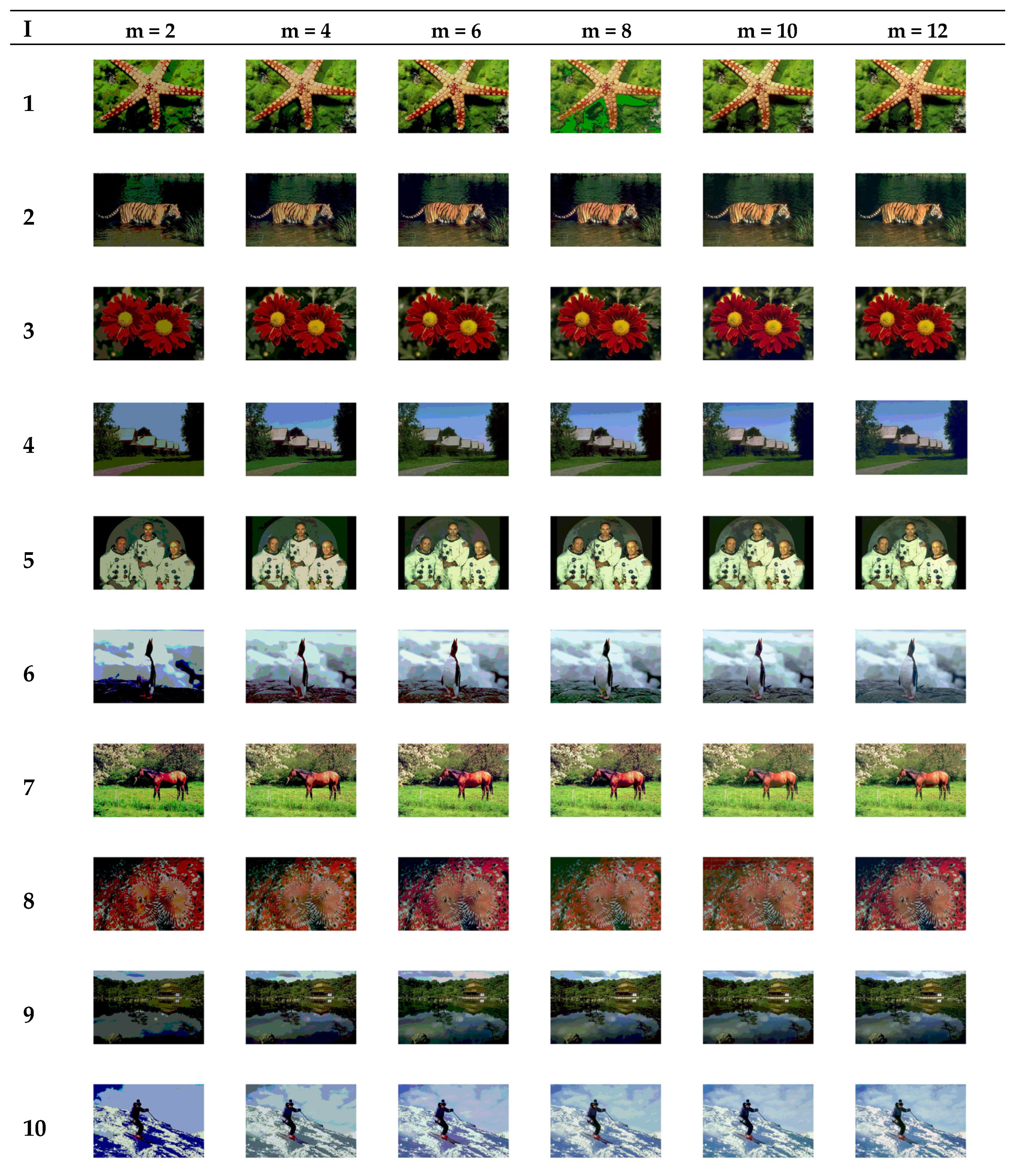
4.3.4. Performance Evaluation Using PSNR, SSIM and FSIM
5. Discussion and Conclusions
Author Contributions
Funding
Data Availability Statement
Conflicts of Interest
References
- Biratu, E.S.; Schwenker, F.; Ayano, Y.M.; Debelee, T.G. A Survey of Brain Tumor Segmentation and Classification Algorithms. J. Imaging 2021, 7, 179. [Google Scholar] [CrossRef] [PubMed]
- Xiong, Y.; Yuan, D.; Li, L.; Shu, X. MFPNet: Mixed Feature Perception Network for Automated Skin Lesion Segmentation. In Pattern Recognition and Computer Vision. PRCV 2024. Lecture Notes in Computer Science; Lin, Z., Cheng, M.-M., He, R., Ubul, K., Silamu, W., Zha, H., Zhou, J., Liu, C.-L., Eds.; Springer: Singapore, 2025; Volume 15044. [Google Scholar] [CrossRef]
- Muhammad, K.; Hussain, T.; Ullah, H.; Del Ser, J.; Rezaei, M.; Kumar, N.; Hijji, M.; Bellavista, P.; de Albuquerque, V.H.C. Vision-Based Semantic Segmentation in Scene Understanding for Autonomous Driving: Recent Achievements, Challenges, and Outlooks. IEEE Trans. Intell. Transp. Syst. 2022, 23, 22694–22715. [Google Scholar] [CrossRef]
- Singh, V.; Misra, A. Detection of plant leaf diseases using image segmentation and soft computing techniques. Inf. Process. Agric. 2017, 4, 41–49. [Google Scholar] [CrossRef]
- Sun, Y.; Bhanu, B. Symmetry integrated region-based image segmentation. In Proceedings of the 2009 IEEE Conference on Computer Vision and Pattern Recognition, Miami, FL, USA, 20–25 June 2009; pp. 826–831. [Google Scholar] [CrossRef]
- Saha, S.; Bandyopadhyay, S. MRI brain image segmentation by fuzzy symmetry based genetic clustering technique. In Proceedings of the 2007 IEEE Congress on Evolutionary Computation, Singapore, 25–28 September 2007; pp. 4417–4424. [Google Scholar] [CrossRef]
- Chen, H.; Qin, Z.; Ding, Y.; Tian, L.; Qin, Z. Brain tumor segmentation with deep convolutional symmetric neural network. Neurocomputing 2020, 392, 305–313. [Google Scholar] [CrossRef]
- Eisham, Z.K.; Haque, M.; Rahman, S.; Nishat, M.M.; Faisal, F.; Islam, M.R. Chimp optimization algorithm in multilevel image thresholding and image clustering. Evol. Syst. 2022, 14, 605–648. [Google Scholar] [CrossRef]
- Kapur, J.N.; Sahoo, P.K.; Wong, A.K.C. A new method for gray-level picture thresholding using the entropy of the histogram. Comput. Vis. Graph. Image Process. 1985, 29, 273–285. [Google Scholar] [CrossRef]
- Otsu, N. A threshold selection method from gray-level histograms. IEEE Trans. Syst. Man Cybern. 1979, 9, 62–66. [Google Scholar] [CrossRef]
- Sezgin, M.; Sankur, B.L. Survey over image thresholding techniques and quantitative performance evaluation. J. Electron. Imaging 2004, 13, 146–168. [Google Scholar]
- Bhandari, A.K.; Kumar, A.; Singh, G.K. Modified artificial bee colony based computationally efficient multilevel thresholding for satellite image segmentation using Kapur’s, Otsu and Tsallis functions. Expert Syst. Appl. 2015, 42, 1573–1601. [Google Scholar] [CrossRef]
- Suresh, S.; Lal, S. An efficient cuckoo search algorithm based multilevel thresholding for segmentation of satellite images using different objective functions. Expert Syst. Appl. 2016, 58, 184–209. [Google Scholar] [CrossRef]
- Pare, S.; Kumar, A.; Bajaj, V.; Singh, G.K. An efficient method for multilevel color image thresholding using cuckoo search algorithm based on minimum cross entropy. Appl. Soft Comput. 2017, 61, 570–592. [Google Scholar] [CrossRef]
- Holland, J.H. Adaptation in Natural and Artificial Systems: An Introductory Analysis with Applications to Biology, Control and Artificial Intelligence; MIT Press: Cambridge, MA, USA, 1992. [Google Scholar]
- Gandomi, A.H.; Yang, X.-S.; Alavi, A.H. Cuckoo search algorithm: A metaheuristic approach to solve structural optimization problems. Eng. Comput. 2013, 29, 17–35. [Google Scholar] [CrossRef]
- Mirjalili, S.; Mirjalili, S.M.; Lewis, A. Grey wolf optimizer. Adv. Eng. Softw. 2014, 69, 46–61. [Google Scholar] [CrossRef]
- Heidari, A.A.; Mirjalili, S.; Faris, H.; Aljarah, I.; Mafarja, M.; Chen, H. Harris hawks optimization: Algorithm and applications. Futur. Gener. Comput. Syst. 2019, 97, 849–872. [Google Scholar] [CrossRef]
- Mirjalili, S. Moth-flame optimization algorithm: A novel nature-inspired heuristic paradigm. Knowl. Based Syst. 2015, 89, 228–249. [Google Scholar] [CrossRef]
- Mirjalili, S. SCA: A Sine Cosine Algorithm for solving optimization problems. Knowl.-Based Syst. 2016, 96, 120–133. [Google Scholar] [CrossRef]
- Mirjalili, S.; Gandomi, A.H.; Mirjalili, S.Z.; Saremi, S.; Faris, H.; Mirjalili, S.M. Salp Swarm Algorithm: A bio-inspired optimizer for engineering design problems. Adv. Eng. Softw. 2017, 114, 163–191. [Google Scholar] [CrossRef]
- Su, H.; Zhao, D.; Yu, F.; Heidari, A.A.; Zhang, Y.; Chen, H.; Li, C.; Pan, J.; Quan, S. Horizontal and vertical search artificial bee colony for image segmentation of COVID-19 X-ray images. Comput. Biol. Med. 2022, 142, 105181. [Google Scholar] [CrossRef]
- Liu, Q.; Li, N.; Jia, H.; Qi, Q.; Abualigah, L. A chimp-inspired remora optimization algorithm for multilevel thresholding image segmentation using cross entropy. Artif. Intell. Rev. 2023, 56, 159–216. [Google Scholar] [CrossRef]
- Sharma, A.; Chaturvedi, R.; Bhargava, A. A novel opposition based improved firefly algorithm for multilevel image segmentation. Multimed. Tools Appl. 2022, 81, 15521–15544. [Google Scholar] [CrossRef]
- Houssein, E.H.; Abdelkareem, D.A.; Emam, M.M.; Hameed, M.A.; Younan, M. An efficient image segmentation method for skin cancer imaging using improved golden jackal optimization algorithm. Comput. Biol. Med. 2022, 149, 106075. [Google Scholar] [CrossRef] [PubMed]
- Gharehchopogh, F.S.; Ibrikci, T. An improved African vultures optimization algorithm using different fitness functions for multi-level thresholding image segmentation. Multimed. Tools Appl. 2023, 83, 16929–16975. [Google Scholar] [CrossRef]
- Kumar, A.; Vishwakarma, A.; Singh, G.K. Multilevel thresholding for crop image segmentation based on recursive minimum cross entropy using a swarm-based technique. Comput. Electron. Agric. 2022, 203, 107488. [Google Scholar] [CrossRef]
- Agrawal, S.; Panda, R.; Choudhury, P.; Abraham, A. Dominant color component and adaptive whale optimization algorithm for multilevel thresholding of color images. Knowl.-Based Syst. 2022, 240, 108172. [Google Scholar] [CrossRef]
- Tan, Z.; Li, K.; Wang, Y. An improved cuckoo search algorithm for multilevel color image thresholding based on modified fuzzy entropy. J. Ambient. Intell. Humaniz. Comput. 2021, 1–14. [Google Scholar] [CrossRef]
- Houssein, E.H.; Mohamed, G.M.; Ibrahim, I.A.; Wazery, Y.M. An efficient multilevel image thresholding method based on improved heap-based optimizer. Sci. Rep. 2023, 13, 9094. [Google Scholar] [CrossRef]
- Wang, Z.; Mo, Y.; Cui, M.; Hu, J.; Lyu, Y.; Oliva, D. An improved golden jackal optimization for multilevel thresholding image segmentation. PLoS ONE 2023, 18, e0285211. [Google Scholar] [CrossRef]
- Abualigah, L.; Al-Okbi, N.K.; Elaziz, M.A.; Houssein, E.H. Boosting Marine Predators Algorithm by Salp Swarm Algorithm for Multilevel Thresholding Image Segmentation. Multimed. Tools Appl. 2022, 81, 16707–16742. [Google Scholar] [CrossRef]
- Swain, M.; Tripathy, T.T.; Panda, R.; Agrawal, S.; Abraham, A. Differential exponential entropy-based multilevel threshold selection methodology for colour satellite images using equilibrium-cuckoo search optimizer. Eng. Appl. Artif. Intell. 2022, 109, 104599. [Google Scholar] [CrossRef]
- Thomas, E.; Kumar, S.N. Harris Hawks Optimization-Based Multilevel Thresholding Segmentation of Magnetic Resonance Brain Images. In International Conference on Communication, Devices and Computing; Springer Nature: Singapore, 2023. [Google Scholar]
- Renugambal, A.; Bhuvaneswari, K.S.; Tamilarasan, A. Hybrid SCCSA: An efficient multilevel thresholding for enhanced image segmentation. Multimed. Tools Appl. 2023, 82, 32711–32753. [Google Scholar] [CrossRef]
- Akay, R.; Saleh, R.A.A.; Farea, S.M.O.; Kanaan, M. Multilevel thresholding segmentation of color plant disease images using metaheuristic optimization algorithms. Neural Comput. Appl. 2021, 34, 1161–1179. [Google Scholar] [CrossRef]
- Akan, T.; Oliva, D.; Feizi-Derakhshi, A.R.; Feizi-Derakhshi, A.R.; Pérez-Cisneros, M.; Bhuiyan, M.A.N. Battle royale optimizer for multi-level image thresholding. J. Supercomput. 2023, 80, 5298–5340. [Google Scholar] [CrossRef]
- Zhang, J.; Zhang, G.; Kong, M.; Zhang, T. SCGJO: A hybrid golden jackal optimization with a sine cosine algorithm for tackling multilevel thresholding image segmentation. Multimed. Tools Appl. 2023, 83, 7681–7719. [Google Scholar] [CrossRef]
- Kang, X.; Hua, C. Multilevel thresholding image segmentation algorithm based on Mumford–Shah model. J. Intell. Syst. 2023, 32, 20220290. [Google Scholar] [CrossRef]
- Wang, C.; Tu, C.; Wei, S.; Yan, L.; Wei, F. MSWOA: A Mixed-Strategy-Based Improved Whale Optimization Algorithm for Multilevel Thresholding Image Segmentation. Electronics 2023, 12, 2698. [Google Scholar] [CrossRef]
- Khishe, M.; Nezhadshahbodaghi, M.; Mosavi, M.R.; Martin, D. A Weighted Chimp Optimization Algorithm. IEEE Access 2021, 9, 158508–158539. [Google Scholar] [CrossRef]
- Khishe, M.; Mosavi, M.R. Chimp optimization algorithm. Expert Syst. Appl. 2020, 149, 113338. [Google Scholar] [CrossRef]
- Kahraman, H.T.; Aras, S.; Gedikli, E. Fitness-distance balance (FDB): A new selection method for meta-heuristic search algorithms. Knowl.-Based Syst. 2020, 190, 105169. [Google Scholar] [CrossRef]
- Orujpour, M.; Feizi-Derakhshi, M.-R.; Akan, T. A multimodal butterfly optimization using fitness-distance balance. Soft Comput. 2023, 27, 17909–17922. [Google Scholar] [CrossRef]
- Ozkaya, B.; Guvenc, U.; Bingol, O. Fitness Distance Balance Based LSHADE Algorithm for Energy Hub Economic Dispatch Problem. IEEE Access 2022, 10, 66770–66796. [Google Scholar] [CrossRef]
- Zheng, K.; Yuan, X.; Xu, Q.; Dong, L.; Yan, B.; Chen, K. Hybrid particle swarm optimizer with fitness-distance balance and individual self-exploitation strategies for numerical optimization problems. Inf. Sci. 2022, 608, 424–452. [Google Scholar] [CrossRef]
- Tang, Z.; Tao, S.; Wang, K.; Lu, B.; Todo, Y.; Gao, S. Chaotic Wind Driven Optimization with Fitness Distance Balance Strategy. Int. J. Comput. Intell. Syst. 2022, 15, 46. [Google Scholar] [CrossRef]
- Liang, J.J.; Suganthan, P.N.; Qu, B.Y.; Gong, D.W.; Yue, C.T. Problem Definitions and Evaluation Criteria for the CEC 2020 Special Session and Competition on Single Objective Bound Constrained Numerical Optimization, Technical Report 201911; Nanyang Technological University: Singapore, 2020.
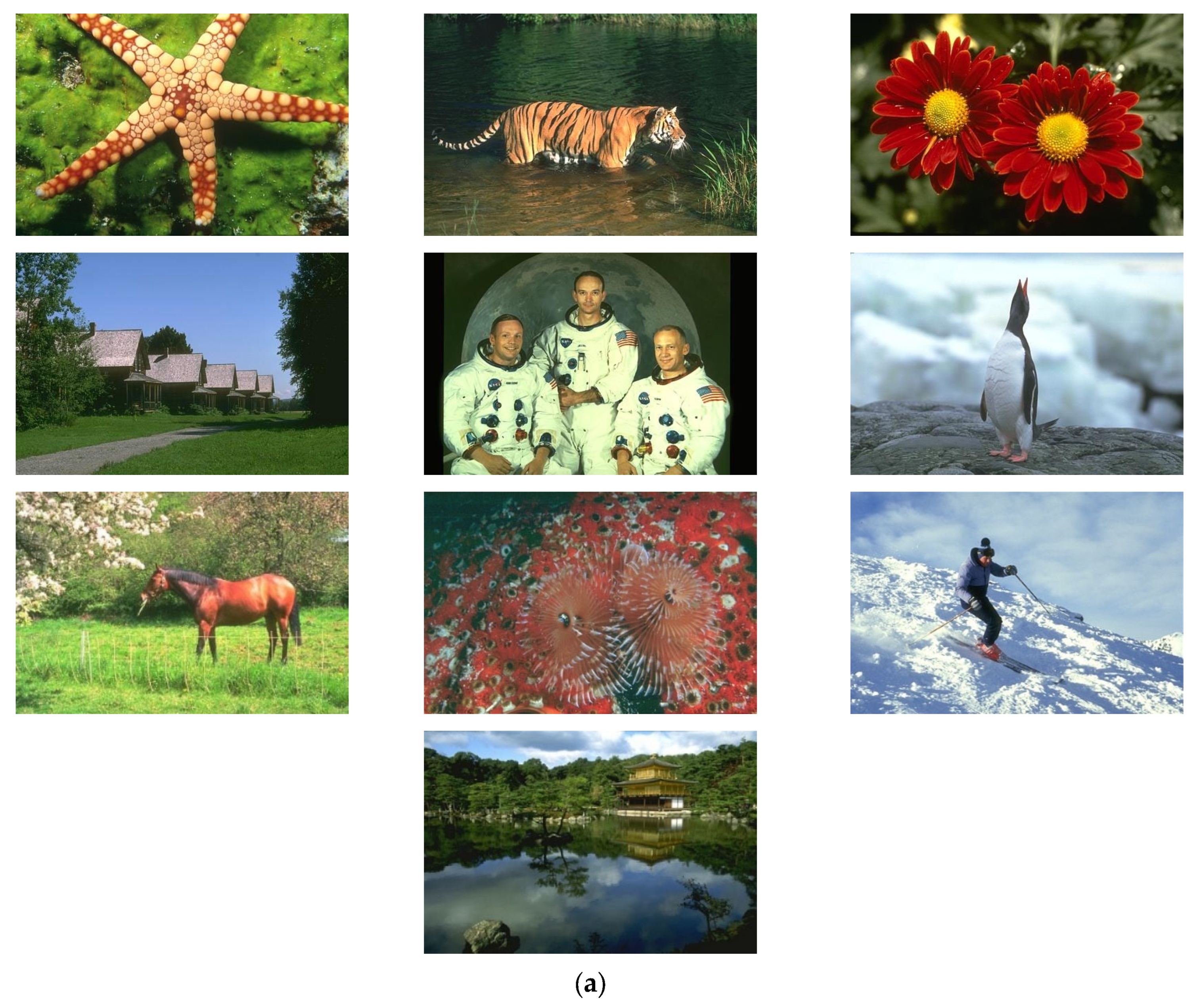
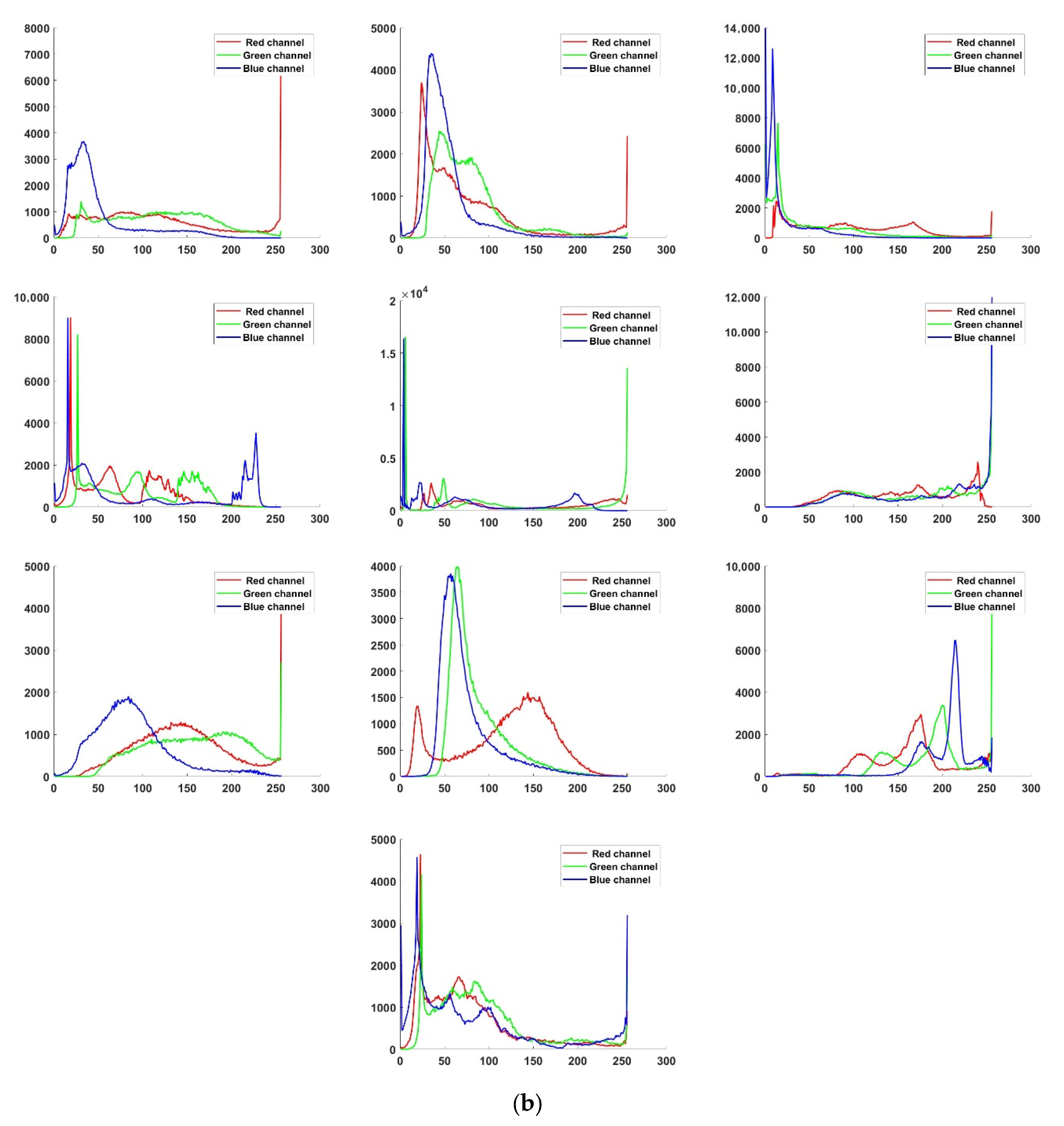
- The Berkeley Segmentation Dataset: Images. Available online: https://www2.eecs.berkeley.edu/Research/Projects/CS/vision/bsds/BSDS300/html/dataset/images.html (accessed on 3 July 2025).

| Algorithm | Explanation | Mathematical Model | |
|---|---|---|---|
| Case-1 | In this case, the proposed development process was achieved by replacing the component in driver equation with FDB method (). | (23) | |
| Case-2 | In this case, the proposed development process was achieved by replacing the component in driver equation with FDB method (). | (24) | |
| Case-3 | In this case, the proposed development process was achieved by replacing the and components in attacker and driver equations, respectively, with FDB method (). | (25) | |
| Case-4 | In this case, the proposed development process was achieved by replacing the and components in attacker and driver equations, respectively, with FDB method (). | (26) | |
| Case-5 | In this case, the proposed development process was achieved by replacing the and components in attacker and driver equations, respectively, with FDB method (). | (27) | |
| Case-6 | In this case, the proposed development process was achieved by replacing the component in attacker and driver equations, respectively, with FDB method (). | (28) | |
| Case-7 | In this case, the proposed development process was achieved by replacing the and components in barrier and driver equations, respectively, with FDB method (). | (29) | |
| Case-8 | In this case, the proposed development process was achieved by replacing the and components in barrier and driver equations, respectively, with FDB method (). | (30) | |
| No. | Function Type | Function Description | |
|---|---|---|---|
| F1 | Unimodal | Shifted and Rotated Bent Cigar Function | 100 |
| F2 | Multimodal Functions | Shifted and Rotated Schwefel’s Function | 1100 |
| F3 | Multimodal Functions | Shifted and Rotated Lunacek bi-Rastrigin Function | 700 |
| F4 | Multimodal Functions | Expanded Rosenbrock’s plus Griewangk’s Function | 1900 |
| F5 | Hybrid Functions | Hybrid Function 1 (N = 3)) | 1700 |
| F6 | Hybrid Functions | Hybrid Function 2 (N = 4) | 1600 |
| F7 | Hybrid Functions | Hybrid Function 3 (N = 5) | 2100 |
| F8 | Composition Functions | Composition Function 1 (N = 3) | 2200 |
| F9 | Composition Functions | Composition Function 2 (N = 4) | 2400 |
| F10 | Composition Functions | Composition Function 3 (N = 5) | 2500 |
| Search range: , D: number of dimensions. (10, 30, 50, 100) | |||
| Algorithm | Dimension = 10 | Dimension = 30 | Dimension = 50 | Dimension = 100 | Mean Rank |
|---|---|---|---|---|---|
| Case-1 | 4.681 | 4.938 | 4.785 | 4.802 | 4.801 5th |
| Case-2 | 4.678 | 4.683 | 4.804 | 4.723 | 4.722 3rd |
| Case-3 | 4.826 | 4.795 | 4.623 | 4.590 | 4.708 2nd |
| Case-4 | 4.864 | 4.709 | 4.697 | 4.492 | 4.690 1st |
| Case-5 | 4.921 | 5.190 | 5.119 | 4.933 | 5.040 7th |
| Case-6 | 5.316 | 5.183 | 5.185 | 5.057 | 5.185 8th |
| Case-7 | 4.897 | 4.842 | 4.697 | 4.852 | 4.822 6th |
| Case-8 | 4.916 | 4.478 | 4.778 | 4.838 | 4.752 4th |
| WChOA | 5.897 | 6.178 | 6.307 | 6.709 | 6.272 9th |
| vs. WChOA +/=/− | Dimension 10 | Dimension 30 | Dimension 50 | Dimension 100 |
|---|---|---|---|---|
| Case-1 | 5_5_0 | 6_4_0 | 6_4_0 | 5_5_0 |
| Case-2 | 5_5_0 | 6_4_0 | 4_6_0 | 7_3_0 |
| Case-3 | 4_6_0 | 5_5_0 | 6_4_0 | 7_3_0 |
| Case-4 | 4_6_0 | 5_5_0 | 5_5_0 | 7_3_0 |
| Case-5 | 5_5_0 | 4_6_0 | 4_6_0 | 6_4_0 |
| Case-6 | 4_5_1 | 4_6_0 | 5_5_0 | 6_4_0 |
| Case-7 | 4_6_0 | 5_5_0 | 6_4_0 | 5_5_0 |
| Case-8 | 4_6_0 | 5_5_0 | 7_3_0 | 5_5_0 |
| Algorithm | Settings |
|---|---|
| WChOA | search agents = 30, …. |
| ABC | colony size = 50, SN = colony size/2, limit = D × SN |
| CS | number of nests = 25, probability = 0.25, beta = 1.5 |
| GWO | number of search agents = 30 |
| HHO | N = 30, Bfid = 1, nD = 10, Jr = 0.25 |
| MFO | number of moths = 30 |
| SCA | number of search agents = 30, a = 2 |
| SSA | salp population size = 30 |
| 3 × 25 Run (RGB), maxFEs = 500 × m, | |||||
| m = 2 | m = 4 | m = 6 | m = 8 | m = 10 | m = 12 |
| Case-2 (6.98) | Case-2 (7.92) | Case-7 (8.03) | Case-8 (8.07) | Case-7 (8.07) | Case-8 (8.22) |
| WChOA (7.60) | WChOA (8.21) | WCHOA (8.19) | WCHOA (8.34) | WCHOA (8.21) | WCHOA (8.33) |
| HHO (9.50) | GWO (8.93) | GWO (8.89) | SCA (8.40) | MFO (8.68) | HHO (8.56) |
| SSA (9.63) | SSA (9.01) | MFO (8.98) | MFO (8.83) | SCA (8.98) | SCA (8.72) |
| SCA (9.73) | MFO (9.21) | SSA (9.37) | GWO (9.13) | SSA (8.99) | SSA (8.79) |
| MFO (9.84) | HHO (9.29) | HHO (9.41) | SSA (9.23) | HHO (9.13) | MFO (9.226) |
| GWO 9.85) | SCA (9.85) | SCA (9.42) | HHO (9.34) | GWO (9.44) | GWO (9.23) |
| ABC (10.33) | CS (9.98) | ABC (9.73) | CS (9.99) | ABC (9.78) | CS (9.53) |
| CS (10.79) | ABC (10.23) | CS (9.92) | ABC (10.26) | CS (10.05) | ABC (10.35) |
| 3 × 25 Run (RGB), maxFEs = 1000 × m, | |||||
| m = 2 | m = 4 | m = 6 | m = 8 | m = 10 | m = 12 |
| WCHOA (7.05) | Case-1 (7.61) | Case-2 (7.89) | Case-8 (8.18) | Case-1 (8.27) | Case-8 (7.84) |
| Case-1 (7.31) | WCHOA (7.72) | WCHOA (8.12) | WCHOA (8.53) | WCHOA (8.33) | WCHOA (8.27) |
| SSA (9.61) | MFO (9.22) | GWO (9.03) | MFO (8.85) | SSA (8.91) | MFO (8.51) |
| SCA (9.89) | GWO (9.30) | MFO (9.11) | GWO (9.00) | HHO (9.069) | SSA (8.73) |
| MFO (10.00) | SCA 9.32) | HHO (9.12) | SCA (9.19) | GWO (9.074) | GWO (9.06) |
| HHO (10.09) | HHO (9.62) | SCA (9.38) | HHO (9.38) | SCA (9.13) | HHO (9.24) |
| GWO (10.14) | SSA (9.77) | SSA (9.79) | CS (9.54) | MFO (9.30) | SCA (9.35) |
| CS (10.67) | ABC (10.15) | CS (9.94) | SSA (9.58) | ABC (9.46) | CS (10.22) |
| ABC (10.80) | CS (10.36) | ABC (10.13) | ABC (10.10) | CS (9.89) | ABC (10.23) |
| 3 × 25 Run (RGB), maxFEs = 500 × m, | |||||
| m = 2 | m = 4 | m = 6 | m = 8 | m = 10 | m = 12 |
| Case-8 (7.80) | Case-2 (8.44) | Case-7 (8.33) | Case-8 (7.98) | Case-2 (8.47) | Case-1 (8.59) |
| WCHOA (8.23) | WCHOA (8.77) | WCHOA (8.61) | SSA (8.28) | WCHOA (8.59) | GWO (8.62) |
| MFO (9.05) | GWO (8.80) | HHO (8.66) | MFO (8.67) | SSA (8.69) | HHO (8.82) |
| GWO (9.22) | MFO (8.83) | SSA (8.86) | GWO (8.73) | MFO (8.83) | WCHOA (8.826) |
| SSA (9.33) | SSA (9.07) | GWO (9.11) | HHO (8.79) | GWO (8.88) | SCA (8.83) |
| SCA (9.63) | HHO (9.15) | SCA (9.11) | WCHOA (8.95) | SCA (8.96) | SSA (9.07) |
| HHO (9.68) | SCA (9.22) | MFO (9.30) | SCA (9.00) | HHO (9.24) | MFO (9.09) |
| CS (10.23) | ABC (9.38) | ABC (9.38) | CS (9.65) | CS (9.57) | ABC (9.27) |
| ABC (10.34) | CS (9.66) | CS (9.68) | ABC (9.70) | ABC (9.59) | CS (9.72) |
| 3 × 25 Run (RGB), maxFEs = 1000 × m, | |||||
| m = 2 | m = 4 | m = 6 | m = 8 | m = 10 | m = 12 |
| Case-2 (7.65) | Case-7 (8.16) | Case-8 (8.48) | Case-2 (8.38) | Case-4 (8.44) | Case-4 (8.18) |
| WCHOA (7.93) | WCHOA (8.22) | WCHOA (8.60) | GWO (8.67) | SCA (8.79) | HHO (8.53) |
| HHO (9.16) | GWO (8.82) | SCA (8.70) | MFO (8.72) | MFO (8.93) | MFO (8.61) |
| SSA (9.41) | MFO (8.91) | GWO (8.82) | SCA (8.73) | HHO (9.02) | GWO (8.71) |
| SCA (9.48) | HHO (8.99) | SSA (8.84) | WCHOA (8.74) | WCHOA (9.14) | WCHOA (8.86) |
| GWO (9.83) | SSA (9.07) | HHO (8.96) | HHO (8.78) | GWO (9.15) | SSA (8.98) |
| MFO (9.95) | ABC (9.41) | MFO (8.97) | SSA (9.17) | SSA (9.22) | SCA (9.33) |
| ABC (10.44) | CS (9.51) | ABC (9.38) | ABC (9.31) | ABC (9.28) | CS (9.49) |
| CS (10.48) | SCA (9.57) | CS 9.99) | CS (9.41) | CS (9.61) | ABC (9.59) |
| m | I | ABC | CS | GWO | HHO | MFO | SCA | SSA | WChOA | Case-1 | Case-2 | Case-3 | Case-4 | Case-5 | Case-6 | Case-7 | Case-8 |
|---|---|---|---|---|---|---|---|---|---|---|---|---|---|---|---|---|---|
| 2 | 1 | 2737.074 | 2725.243 | 2743.743 | 2739.341 | 2737.367 | 2735.023 | 2742.085 | 2752.066 | 2748.824 | 758.227 | 2742.976 | 2746.675 | 2741.095 | 2733.923 | 2743.837 | 2744.737 |
| 2 | 1546.111 | 1542.659 | 1543.179 | 1550.087 | 1549.543 | 1542.648 | 1550.242 | 1558.874 | 1562.89 | 1560.921 | 1557.5 | 1556.029 | 1555.361 | 1545.926 | 1557.683 | 1558.725 | |
| 3 | 2045.823 | 2048.159 | 2052.438 | 2055.056 | 2056.045 | 2058.083 | 2056.986 | 2063.669 | 2069.752 | 2060.543 | 2064.757 | 2063.925 | 2063.697 | 2062.156 | 2060.129 | 2064.917 | |
| 4 | 3751.211 | 3750.514 | 3746.45 | 3755.181 | 3745.171 | 3753.348 | 3750.586 | 3768.945 | 3767.619 | 3769.786 | 3772.374 | 3767.559 | 3767.873 | 3765.901 | 3764.98 | 3769.406 | |
| 5 | 6543.776 | 6539.734 | 6556.53 | 6553.129 | 6548.085 | 6555.473 | 6550.013 | 6572.956 | 6572.608 | 6573.75 | 6572.767 | 6565.286 | 6563.162 | 6564.433 | 6576.648 | 6566.533 | |
| 6 | 3410.207 | 3432.674 | 3433.317 | 3432.827 | 3422.742 | 3432.178 | 3426.886 | 3432.669 | 3437.171 | 3438.64 | 3422.988 | 3429.121 | 3427.679 | 3425.944 | 3429.048 | 3430.714 | |
| 7 | 2001.345 | 1992.559 | 2006.84 | 2006.68 | 2006.063 | 2002.733 | 2008.456 | 2014.906 | 2011.195 | 2009.464 | 2015.995 | 2010.7 | 2010.275 | 2009.741 | 2005.913 | 2016.538 | |
| 8 | 1332.685 | 1325.152 | 1328.754 | 1339.794 | 1332.781 | 1337.124 | 1338.239 | 1346.524 | 1349.764 | 1346.32 | 1349.134 | 1348.85 | 1341.322 | 1345.048 | 1346.207 | 1349.081 | |
| 9 | 3078.593 | 3086.274 | 3090.238 | 3097.18 | 3090.702 | 3088.602 | 3096.844 | 3108.937 | 3099.905 | 3107.093 | 3096.787 | 3099.8 | 3099.324 | 3099.298 | 3095.716 | 3097.638 | |
| 10 | 1525.829 | 1500.797 | 1526.837 | 1531.625 | 1508.113 | 1522.823 | 1522.144 | 1532.401 | 1532.89 | 1529.045 | 1523.838 | 1524.909 | 1533.122 | 1526.415 | 1530.328 | 1529.312 | |
| 4 | 1 | 2971.224 | 2983.725 | 2978.576 | 2979.185 | 2982.445 | 2979.029 | 2979.672 | 2980.495 | 2985.098 | 2983.454 | 2978.855 | 2984.145 | 2983.573 | 2982.657 | 2983.677 | 2985.035 |
| 2 | 1685.928 | 1685.786 | 1690.94 | 1690.277 | 1690.988 | 1684.644 | 1691.281 | 1691.914 | 1692.159 | 1694.731 | 1693.811 | 1690.774 | 1695.597 | 1688.21 | 1690.137 | 1691.956 | |
| 3 | 2237.984 | 2233.492 | 2242.192 | 2236.82 | 2242.401 | 2238.648 | 2242.114 | 2246.91 | 2251.695 | 2247.267 | 2243.703 | 2246.085 | 2245.638 | 2245.366 | 2242.789 | 2247.555 | |
| 4 | 3907.647 | 3904.117 | 3915.465 | 3916.674 | 3905.069 | 3911.686 | 3916.22 | 3916.376 | 3916.036 | 3920.918 | 3919.852 | 3918.136 | 3920.576 | 3913.992 | 3920.143 | 3919.481 | |
| 5 | 6850.046 | 6856.642 | 6856.163 | 6861.359 | 6856.216 | 6858.982 | 6857.505 | 6865.578 | 6864.933 | 6866.469 | 6862.937 | 6863.268 | 6860.461 | 6854.138 | 6860.196 | 6863.986 | |
| 6 | 3626.963 | 3621.681 | 3635.886 | 3629.191 | 3635.181 | 3634.584 | 3630.871 | 3639.573 | 3631.285 | 3632.235 | 3639.309 | 3630.197 | 3634.974 | 3633.786 | 3636.253 | 3640.083 | |
| 7 | 2215.266 | 2220.331 | 2228.699 | 2224.114 | 2233.559 | 2220.861 | 2220.534 | 2226.323 | 2229.603 | 2222.014 | 2222.431 | 2225.457 | 2223.379 | 2229.035 | 2230.55 | 2221.228 | |
| 8 | 1458.24 | 1460.839 | 1466.011 | 1461.55 | 1462.692 | 1461.551 | 1465.346 | 1466.807 | 1462.093 | 1463.385 | 1462.209 | 1464.689 | 1467.757 | 1458.666 | 1468.058 | 1461.075 | |
| 9 | 3326.803 | 3329.522 | 3340.704 | 3340.955 | 3336.021 | 3336.222 | 3341.613 | 3342.281 | 3338.818 | 3350.156 | 3340.224 | 3340.15 | 3335.643 | 3334.665 | 3344.094 | 3341.944 | |
| 10 | 1731.037 | 1725.522 | 1732.67 | 1728.978 | 1733.961 | 1735.643 | 1739.335 | 1735.071 | 1740.234 | 1731.957 | 1731.666 | 1737.891 | 1736.247 | 1739.74 | 1742.006 | 1746.334 | |
| 6 | 1 | 3055.786 | 3062.076 | 3062.298 | 3059.377 | 3060.01 | 3057.887 | 3059.611 | 3067.026 | 3062.175 | 3065.018 | 3060.077 | 3061.563 | 3064.167 | 3064.047 | 3062.819 | 3064.734 |
| 2 | 1739.541 | 1736.057 | 1743.046 | 1740.114 | 1740.816 | 1740.505 | 1738.122 | 1740.503 | 1741.137 | 1739.936 | 1742.39 | 1743.033 | 1736.743 | 1738.72 | 1741.42 | 1740.668 | |
| 3 | 2300.056 | 2297.708 | 2301.462 | 2302.265 | 2304.24 | 2302.317 | 2301.682 | 2302.744 | 2305.403 | 2307.668 | 2305.133 | 2306.693 | 2300.929 | 2308.062 | 2307.642 | 2305.348 | |
| 4 | 3968.216 | 3966.064 | 3970.711 | 3969.996 | 3965.829 | 3967.566 | 3967.846 | 3973.705 | 3969.814 | 3968.732 | 3970.132 | 3970.526 | 3969.221 | 3968.834 | 3971.435 | 3967.14 | |
| 5 | 6944.81 | 6946.51 | 6949.056 | 6948.293 | 6953.987 | 6950.394 | 6951.48 | 6952.411 | 6953.982 | 6951.883 | 6950.96 | 6948.6 | 6952.184 | 6948.545 | 6956.471 | 6952.526 | |
| 6 | 3703.885 | 3707.077 | 3707.834 | 3702.849 | 3706.919 | 3709.819 | 3706.175 | 3709.408 | 3707.619 | 3709.916 | 3710.537 | 3707.324 | 3708.627 | 3710.73 | 3709.275 | 3708.092 | |
| 7 | 2303.496 | 2297.185 | 2304.373 | 2304.355 | 2303.958 | 2303.739 | 2301.594 | 2304.913 | 2303.75 | 2302.027 | 2305.436 | 2303.754 | 2306.8 | 2305.37 | 2298.706 | 2307.224 | |
| 8 | 1505.397 | 1507.466 | 1512.165 | 1512.44 | 1509.612 | 1511.83 | 1509.776 | 1513.262 | 1511.194 | 1508.625 | 1512.027 | 1510.219 | 1511.149 | 1511.152 | 1511.32 | 1511.749 | |
| 9 | 3419.025 | 3421.206 | 3424.437 | 3422.984 | 3426.666 | 3422.367 | 3422.771 | 3427.851 | 3429.736 | 3427.156 | 3424.266 | 3425.246 | 3427.52 | 3424.029 | 3427.858 | 3428.033 | |
| 10 | 1792.242 | 1791.979 | 1796.248 | 1797.419 | 1794.984 | 1792.366 | 1796.761 | 1795.846 | 1794.564 | 1800.367 | 1797.849 | 1794.258 | 1795.875 | 1797.854 | 1795.282 | 1794.056 | |
| 8 | 1 | 3095.035 | 3094.788 | 3100.935 | 3100.012 | 3103.595 | 3099.656 | 3100.506 | 3098.546 | 3104.124 | 3100.637 | 3098.626 | 3099.479 | 3101.677 | 3101.74 | 3104.208 | 3100.35 |
| 2 | 1763.523 | 1763.879 | 1764.596 | 1764.643 | 1767.469 | 1768.115 | 1764.392 | 1768.653 | 1768.017 | 1767.328 | 1765.518 | 1765.958 | 1766.287 | 1767.216 | 1765.996 | 1768.691 | |
| 3 | 2330.243 | 2332.263 | 2334.553 | 2333.814 | 2333.914 | 2335.018 | 2334.367 | 2335.825 | 2332.99 | 2335.402 | 2335.729 | 2334.178 | 2333.14 | 2335.624 | 2334.013 | 2334.405 | |
| 4 | 3993.417 | 3994.206 | 3993.94 | 3994.909 | 3993.251 | 3997.008 | 3996.942 | 3999.81 | 3998.207 | 3999.083 | 3997.443 | 3997.645 | 3995.869 | 3994.276 | 3996.613 | 3998.257 | |
| 5 | 6992.46 | 6994.43 | 6995.409 | 6994.536 | 6995.865 | 6997.45 | 6995.604 | 6993.495 | 6997.185 | 6993.848 | 6994.644 | 6996.019 | 6993.927 | 6996.418 | 6997.189 | 6997.663 | |
| 6 | 3742.932 | 3738.304 | 3742.176 | 3745.083 | 3744.734 | 3747.146 | 3742.216 | 3742.347 | 3742.419 | 3739.728 | 3744.674 | 3744.946 | 3742 | 3747.931 | 3745.343 | 3743.693 | |
| 7 | 2341.433 | 2337.658 | 2341.707 | 2340.95 | 2342.599 | 2343.816 | 2343.457 | 2341.77 | 2341.306 | 2345.089 | 2340.648 | 2341.969 | 2341.934 | 2339.032 | 2341.941 | 2343.293 | |
| 8 | 1532.37 | 1533.489 | 1533.219 | 1532.896 | 1535.076 | 1534.259 | 1536.2 | 1536.904 | 1535.819 | 1536.228 | 1536.754 | 1536.637 | 1533.963 | 1533.872 | 1534.513 | 1535.599 | |
| 9 | 3462.031 | 3461.852 | 3464.573 | 3466.318 | 3461.814 | 3462.475 | 3464.669 | 3461.062 | 3465.976 | 3463.881 | 3465.466 | 3463.109 | 3465.688 | 3463 | 3464.724 | 3463.39 | |
| 10 | 1823.205 | 1822.047 | 1825.318 | 1822.844 | 1823.57 | 1826.354 | 1823.671 | 1823.238 | 1824.776 | 1823.024 | 1824.77 | 1824.682 | 1823.968 | 1822.874 | 1824.185 | 1823.903 | |
| 10 | 1 | 3121.272 | 3120.716 | 3121.541 | 3122.446 | 3121.88 | 3123.461 | 3121.707 | 3122.548 | 3123.24 | 3124.93 | 3122.275 | 3123.788 | 3123.813 | 3122.623 | 3125.303 | 3124.233 |
| 2 | 1780.889 | 1779.301 | 1780.672 | 1781.553 | 1781.717 | 1779.962 | 1780.486 | 1782.688 | 1780.872 | 1781.24 | 1781.569 | 1781.722 | 1779.26 | 1782.714 | 1781.475 | 1782.744 | |
| 3 | 2349.223 | 2347.22 | 2349.941 | 2349.661 | 2350.596 | 2351.171 | 2349.778 | 2352.851 | 2350.929 | 2352.054 | 2350.112 | 2351.156 | 2351.022 | 2351.174 | 2352.244 | 2351.718 | |
| 4 | 4010.342 | 4010.753 | 4012.625 | 4011.558 | 4012.929 | 4012.716 | 4013.307 | 4013.326 | 4012.187 | 4011.648 | 4014.059 | 4013.29 | 4010.777 | 4012.077 | 4013.891 | 4013.239 | |
| 5 | 7016.677 | 7017.247 | 7018.761 | 7019.45 | 7020.418 | 7018.466 | 7019.57 | 7020.04 | 7018.951 | 7019.892 | 7019.9 | 7020.678 | 7020.031 | 7018.165 | 7020.202 | 7018.861 | |
| 6 | 3764.082 | 3767.565 | 3766.572 | 3765.698 | 3764.905 | 3764.871 | 3768.077 | 3764.142 | 3765.857 | 3764.868 | 3766.76 | 3766.391 | 3765.913 | 3764.814 | 3766.928 | 3765.589 | |
| 7 | 2363.542 | 2361.786 | 2366.986 | 2365.115 | 2365.012 | 2365.636 | 2365.319 | 2367.344 | 2366.109 | 2364.133 | 2365.797 | 2366.46 | 2362.534 | 2368.323 | 2364.999 | 2365.382 | |
| 8 | 1549.772 | 1546.985 | 1550.604 | 1550.507 | 1550.854 | 1551.823 | 1548.698 | 1552.82 | 1551.89 | 1549.949 | 1550.952 | 1549.48 | 1551.613 | 1549.012 | 1551.665 | 1550.676 | |
| 9 | 3482.569 | 3485.255 | 3485.294 | 3486.925 | 3486.103 | 3485.139 | 3485.89 | 3487.332 | 3485.683 | 3485.421 | 3484.755 | 3487.011 | 3486.388 | 3484.586 | 3486.593 | 3485.943 | |
| 10 | 1841.121 | 1839.201 | 1841.381 | 1841.749 | 1840.399 | 1840.823 | 1839.551 | 1840.796 | 1840.817 | 1840.762 | 1839.598 | 1838.908 | 1839.984 | 1839.928 | 1839.385 | 1842.901 | |
| 12 | 1 | 3136.007 | 3137.837 | 3137.857 | 3136.9 | 3138.668 | 3138.144 | 3137.766 | 3139.396 | 3137.933 | 3137.861 | 3136.487 | 3137.712 | 3137.715 | 3137.082 | 3138.769 | 3138.984 |
| 2 | 1788.918 | 1789.947 | 1789.865 | 1791.464 | 1790.576 | 1790.157 | 1790.615 | 1791.131 | 1791.84 | 1791.068 | 1789.69 | 1791.593 | 1790.929 | 1791.854 | 1791.904 | 1791.554 | |
| 3 | 2358.881 | 2360.723 | 2360.519 | 2361.172 | 2361.73 | 2361.348 | 2362.522 | 2363.326 | 2362.441 | 2363.241 | 2362.423 | 2361.651 | 2361.495 | 2361.488 | 2362.595 | 2361.647 | |
| 4 | 4021.542 | 4021.101 | 4023.276 | 4023.616 | 4021.452 | 4022.395 | 4023.176 | 4023.792 | 4022.839 | 4021.872 | 4022.023 | 4023.028 | 4023.627 | 4022.798 | 4024.05 | 4024.98 | |
| 5 | 7031.876 | 7033.484 | 7033.18 | 7035.353 | 7032.047 | 7035.917 | 7034.202 | 7032.981 | 7034.485 | 7033.429 | 7033.632 | 7032.504 | 7033.894 | 7034.956 | 7033.989 | 7033.885 | |
| 6 | 3778.532 | 3779.473 | 3779.162 | 3779.449 | 3779.565 | 3779.341 | 3778.395 | 3780.279 | 3778.271 | 3778.942 | 3778.744 | 3779.472 | 3778.63 | 3777.83 | 3780.363 | 3779.821 | |
| 7 | 2378.585 | 2378.113 | 2379.155 | 2379.194 | 2381.583 | 2381.161 | 2379.665 | 2379.437 | 2379.498 | 2381.203 | 2380.351 | 2378.184 | 2379.641 | 2380.059 | 2381.388 | 2379.248 | |
| 8 | 1557.726 | 1559.154 | 1560.626 | 1560.37 | 1559.783 | 1560.107 | 1561.226 | 1561.398 | 1558.858 | 1560.875 | 1560.791 | 1560.69 | 1560.379 | 1561.393 | 1561.181 | 1559.775 | |
| 9 | 3499.918 | 3500.526 | 3500.897 | 3501.652 | 3501.318 | 3499.199 | 3500.579 | 3500.413 | 3499.358 | 3500.897 | 3501.214 | 3500.387 | 3501.753 | 3499.855 | 3501.595 | 3500.624 | |
| 10 | 1848.916 | 1850.436 | 1851.596 | 1851.921 | 1851.159 | 1851.458 | 1852.321 | 1852.37 | 1851.271 | 1850.858 | 1851.481 | 1852.153 | 1851.102 | 1850.839 | 1850.91 | 1849.552 |
| m | I | ABC | CS | GWO | HHO | MFO | SCA | SSA | WChOA | Case-1 | Case-2 | Case-3 | Case-4 | Case-5 | Case-6 | Case-7 | Case-8 |
|---|---|---|---|---|---|---|---|---|---|---|---|---|---|---|---|---|---|
| 2 | 1 | 2728.046 | 2736.835 | 2735.819 | 2738.899 | 2732.252 | 2743.27 | 2748.984 | 2750.304 | 2751.112 | 2753.223 | 2751.062 | 2744.249 | 2744.117 | 2748.843 | 2751.934 | 2748.661 |
| 2 | 1541.264 | 1543.551 | 1553.007 | 1542.008 | 1546.289 | 1544.833 | 1547.862 | 1566.518 | 1560 | 1564.981 | 1558.983 | 1562.899 | 1558.124 | 1554.514 | 1559.679 | 1562.125 | |
| 3 | 2045.685 | 2039.071 | 2055.435 | 2049.221 | 2054.039 | 2053.009 | 2052.089 | 2069.108 | 2071.535 | 2065.321 | 2063.702 | 2070.788 | 2062.614 | 2067.042 | 2064.544 | 2064.917 | |
| 4 | 3748.363 | 3747.132 | 3756.105 | 3763.88 | 3756.725 | 3758.588 | 3761.66 | 3777.123 | 3769.923 | 3765.023 | 3771.937 | 3766.127 | 3764.552 | 3764.588 | 3767.747 | 3772.434 | |
| 5 | 6538.647 | 6541.102 | 6548.044 | 6554.843 | 6551.463 | 6560.329 | 6562.061 | 6577.023 | 6574.494 | 6572.791 | 6561.217 | 6567.042 | 6566.947 | 6568.381 | 6573.875 | 6575.547 | |
| 6 | 3418.88 | 3428.078 | 3425.07 | 3424.068 | 3423.448 | 3437.035 | 3431.321 | 3433.769 | 3434.632 | 3425.304 | 3442.465 | 3430.343 | 3434.823 | 3434.983 | 3434.992 | 3433.11 | |
| 7 | 1998.971 | 1993.185 | 2001.735 | 1995.327 | 2015.309 | 2011.661 | 2004.819 | 2018.947 | 2014.765 | 2010.078 | 2019.249 | 2009.592 | 2013.035 | 2004.64 | 2015.367 | 2023.932 | |
| 8 | 1333.447 | 1338.047 | 1342.042 | 1342.825 | 1340.98 | 1338.311 | 1336.657 | 1345.354 | 1346.992 | 1350.59 | 1342.185 | 1344.259 | 1348.665 | 1336.141 | 1350.515 | 1351.343 | |
| 9 | 3076.526 | 3074.3 | 3092.04 | 3093.225 | 3082.186 | 3082.65 | 3080.201 | 3108.386 | 3102.983 | 3102.363 | 3100.289 | 3108.197 | 3104.625 | 3094.063 | 3098.907 | 3103.495 | |
| 10 | 1512.576 | 1520.529 | 1522.59 | 1531.779 | 1528.389 | 1529.76 | 1528.472 | 1527.622 | 1529.597 | 1530.715 | 1528.477 | 1534.044 | 1531.255 | 1541.085 | 1528.88 | 1529.634 | |
| 4 | 1 | 2968.877 | 2974.673 | 2976.953 | 2982.646 | 2983.781 | 2983.182 | 2974.886 | 2986.18 | 2993.527 | 2983.145 | 2985.545 | 2979.449 | 2985.497 | 2990.744 | 2984.501 | 2989.566 |
| 2 | 1685.734 | 1684.697 | 1691.253 | 1688.241 | 1688.154 | 1685.925 | 1688.085 | 1692.083 | 1692.318 | 1693.647 | 1688.929 | 1690.528 | 1689.897 | 1694.252 | 1690.332 | 1692.058 | |
| 3 | 2236.763 | 2233.671 | 2239.522 | 2237.048 | 2239.533 | 2243.753 | 2241.44 | 2247.71 | 2251.86 | 2244.449 | 2246.807 | 2243.106 | 2241.359 | 2241.43 | 2239.921 | 2249.022 | |
| 4 | 3911.946 | 3906.841 | 3913.986 | 3912.154 | 3913.167 | 3914.514 | 3910.033 | 3922.988 | 3918.909 | 3918.289 | 3915.913 | 3922.249 | 3918.58 | 3916.518 | 3921.51 | 3921.867 | |
| 5 | 6853.341 | 6853.016 | 6857.619 | 6859.257 | 6860.216 | 6856.958 | 6851.583 | 6870.819 | 6870.554 | 6869.962 | 6867.785 | 6865.297 | 6859.28 | 6859.328 | 6860.541 | 6864.823 | |
| 6 | 3622.164 | 3628.469 | 3632.114 | 3629.386 | 3631.182 | 3636.282 | 3632.784 | 3634.409 | 3639.17 | 3632.699 | 3635.723 | 3626.903 | 3632.451 | 3630.29 | 3628.696 | 3629.595 | |
| 7 | 2223.086 | 2220.79 | 2221.21 | 2218.413 | 2230.996 | 2229.773 | 2225.54 | 2231.388 | 2226.721 | 2232.232 | 2225.85 | 2227.68 | 2228.391 | 2224.434 | 2225.59 | 2228.059 | |
| 8 | 1460.392 | 1453.18 | 1462.304 | 1456.405 | 1464.13 | 1460.032 | 1465.229 | 1465.837 | 1463.322 | 1465.049 | 1463.708 | 1462.694 | 1462.984 | 1464.793 | 1467.923 | 1470.102 | |
| 9 | 3334.496 | 3335.009 | 3336.26 | 3342.41 | 3336.526 | 3332.321 | 3332.07 | 3346.039 | 3345.475 | 3343.608 | 3338.967 | 3337.257 | 3339.679 | 3340.703 | 3342.745 | 3343.647 | |
| 10 | 1731.641 | 1732.62 | 1739.704 | 1738.475 | 1734.856 | 1734.896 | 1738.816 | 1736.581 | 1737.571 | 1739.48 | 1739.4 | 1735.278 | 1740.574 | 1734.675 | 1733.197 | 1740.018 | |
| 6 | 1 | 3054.89 | 3057.875 | 3065.102 | 3060.355 | 3065.534 | 3058.264 | 3058.435 | 3064.305 | 3062.155 | 3060.906 | 3065.791 | 3065.027 | 3063.015 | 3059.596 | 3061.147 | 3062.069 |
| 2 | 1736.295 | 1740.601 | 1741.567 | 1742.609 | 1741.826 | 1738.128 | 1736.916 | 1741.491 | 1742.811 | 1743.101 | 1742.887 | 1739.93 | 1740.656 | 1740.016 | 1740.365 | 1741.52 | |
| 3 | 2297.228 | 2298.316 | 2299.478 | 2300.546 | 2303.911 | 2303.289 | 2302.267 | 2307.601 | 2306.669 | 2309.762 | 2304.063 | 2305.343 | 2305.631 | 2304.557 | 2306.897 | 2304.655 | |
| 4 | 3966.832 | 3966.346 | 3968.78 | 3968.852 | 3965.158 | 3968.234 | 3967.571 | 3971.748 | 3971.597 | 3973.789 | 3970.312 | 3971.821 | 3971.719 | 3970.195 | 3971.47 | 3973.35 | |
| 5 | 6948.413 | 6946.323 | 6953.707 | 6951.962 | 6949.013 | 6952.838 | 6951.862 | 6958.564 | 6952.067 | 6955.2 | 6956.26 | 6955.716 | 6947.41 | 6954.764 | 6955.349 | 6955.144 | |
| 6 | 3704.839 | 3703.534 | 3707.762 | 3706.617 | 3708.863 | 3710.317 | 3706.395 | 3707.58 | 3708.317 | 3706.599 | 3707.531 | 3704.282 | 3708.052 | 3706.703 | 3704.996 | 3708.614 | |
| 7 | 2299.587 | 2302.118 | 2304.125 | 2302.648 | 2302.855 | 2300.734 | 2303.164 | 2306.07 | 2307.361 | 2304.45 | 2305.295 | 2306.147 | 2303.055 | 2301.439 | 2302.757 | 2301.506 | |
| 8 | 1507.623 | 1505.338 | 1511.008 | 1509.325 | 1513.302 | 1508.243 | 1509.08 | 1513.86 | 1509.119 | 1511.701 | 1508.891 | 1510.77 | 1507.269 | 1508.652 | 1512.774 | 1511.701 | |
| 9 | 3418.785 | 3419.915 | 3419.67 | 3423.655 | 3421.695 | 3422.716 | 3421.299 | 3428.2 | 3423.16 | 3423.516 | 3425.031 | 3420.209 | 3425.477 | 3423.809 | 3422.04 | 3426.303 | |
| 10 | 1791.085 | 1795.063 | 1797.006 | 1794.699 | 1797.044 | 1795.819 | 1795.145 | 1796.587 | 1795.566 | 1798.723 | 1798.105 | 1799.672 | 1792.64 | 1796.022 | 1796.409 | 1792.647 | |
| 8 | 1 | 3095.424 | 3098.226 | 3096.092 | 3097.604 | 3102.578 | 3099.541 | 3099.191 | 3099.212 | 3101.358 | 3101.778 | 3100.179 | 3100.502 | 3102.252 | 3099.098 | 3101.87 | 3100.961 |
| 2 | 1763.605 | 1764.15 | 1765.118 | 1763.981 | 1764.757 | 1766.239 | 1764.589 | 1766.657 | 1766.214 | 1766.362 | 1767.323 | 1766.702 | 1767.332 | 1767.677 | 1766.73 | 1767.469 | |
| 3 | 2331.683 | 2332.329 | 2336.407 | 2333.429 | 2333.353 | 2332.681 | 2330.897 | 2334.925 | 2335.595 | 2335.206 | 2334.794 | 2335.313 | 2331.837 | 2333.505 | 2335.347 | 2335.138 | |
| 4 | 3991.394 | 3993.546 | 3996.526 | 3994.596 | 3995.894 | 3995.08 | 3993.947 | 3998.584 | 3996.09 | 3995.683 | 3994.939 | 3997.878 | 3995.456 | 3996.091 | 3997.743 | 3998.184 | |
| 5 | 6994.574 | 6992.489 | 6996.982 | 6995.766 | 6996.97 | 6996.545 | 6995.52 | 6996.596 | 6998.921 | 6995.723 | 6995.579 | 6996.429 | 6994.3 | 6996.624 | 6996.008 | 6996.598 | |
| 6 | 3740.619 | 3743.201 | 3744.652 | 3747.414 | 3742.679 | 3745.083 | 3742.676 | 3745.304 | 3746.505 | 3743.033 | 3742.877 | 3744.669 | 3741.516 | 3742.274 | 3745.246 | 3744.463 | |
| 7 | 2338.008 | 2339.88 | 2341.908 | 2341.752 | 2340.785 | 2343.072 | 2344.421 | 2343.893 | 2344.684 | 2344.975 | 2344.928 | 2343.454 | 2339.125 | 2339.513 | 2343.181 | 2342.491 | |
| 8 | 1532.206 | 1534.454 | 1535.469 | 1534.594 | 1536.051 | 1536.161 | 1533.073 | 1534.429 | 1534.321 | 1534.774 | 1534.544 | 1535.912 | 1535.287 | 1535.801 | 1535.95 | 1535.511 | |
| 9 | 3460.832 | 3461.665 | 3461.833 | 3464.059 | 3465.007 | 3463.435 | 3460.846 | 3464.962 | 3464.063 | 3464.794 | 3464.007 | 3464.592 | 3463.611 | 3459.917 | 3463.195 | 3462.235 | |
| 10 | 1821.58 | 1823.373 | 1825.424 | 1823.769 | 1823.732 | 1823.699 | 1823.89 | 1826.243 | 1824.103 | 1824.848 | 1822.675 | 1822.179 | 1823.944 | 1824.598 | 1821.639 | 1825.766 | |
| 10 | 1 | 3121.566 | 3121.436 | 3122.419 | 3123.941 | 3122.662 | 3123.408 | 3122.736 | 3122.229 | 3125.366 | 3124.473 | 3122.204 | 3123.704 | 3125.035 | 3123.791 | 3122.537 | 3124.241 |
| 2 | 1779.86 | 1778.508 | 1780.32 | 1781.454 | 1780.51 | 1780.512 | 1781.793 | 1781.902 | 1781.122 | 1782.374 | 1781.871 | 1780.933 | 1781.002 | 1780.946 | 1780.107 | 1781.327 | |
| 3 | 2348.292 | 2350.154 | 2350.028 | 2348.608 | 2350.075 | 2349.618 | 2349.901 | 2352.94 | 2351.65 | 2352.243 | 2351.126 | 2351.07 | 2352.178 | 2351.473 | 2351.447 | 2351.905 | |
| 4 | 4011.765 | 4010.708 | 4012.009 | 4012.243 | 4012.024 | 4012.82 | 4011.999 | 4013.106 | 4013.321 | 4013.07 | 4013.452 | 4013.395 | 4013.246 | 4011.017 | 4013.645 | 4012.578 | |
| 5 | 7018.332 | 7016.6 | 7018.802 | 7020.395 | 7019.052 | 7018.817 | 7019.594 | 7019.27 | 7018.496 | 7018.313 | 7017.208 | 7019.206 | 7017.496 | 7019.534 | 7018.535 | 7019.683 | |
| 6 | 3765.221 | 3765.084 | 3766.547 | 3764.597 | 3764.329 | 3765.063 | 3766.101 | 3764.879 | 3766.703 | 3767.271 | 3766.753 | 3766.111 | 3763.796 | 3764.821 | 3767.254 | 3767.566 | |
| 7 | 2362.372 | 2364.721 | 2367.784 | 2365.264 | 2367.074 | 2365.771 | 2363.436 | 2366.816 | 2364.538 | 2366.595 | 2365.153 | 2365.298 | 2364.94 | 2364.768 | 2366.19 | 2365.625 | |
| 8 | 1547.35 | 1548.857 | 1550.523 | 1549.75 | 1550.339 | 1548.436 | 1550.902 | 1548.917 | 1550.333 | 1551.165 | 1549.411 | 1550.627 | 1548.317 | 1550.911 | 1550.535 | 1550.003 | |
| 9 | 3484.584 | 3486.2 | 3487.555 | 3486.881 | 3486.499 | 3486.478 | 3488.178 | 3486.453 | 3485.418 | 3487.519 | 3487.666 | 3485.411 | 3485.499 | 3486.559 | 3486.85 | 3486.332 | |
| 10 | 1840.401 | 1841.179 | 1839.402 | 1839.981 | 1840.279 | 1841.144 | 1840.132 | 1840.866 | 1842.475 | 1840.578 | 1839.741 | 1840.352 | 1840.648 | 1840.58 | 1839.715 | 1838.935 | |
| 12 | 1 | 3134.44 | 3136.6 | 3136.688 | 3138.253 | 3139.368 | 3137.47 | 3137.295 | 3137.719 | 3137.197 | 3138.016 | 3137.149 | 3136.706 | 3136.78 | 3137.356 | 3137.76 | 3138.711 |
| 2 | 1791.053 | 1790.06 | 1792.763 | 1791.236 | 1792.344 | 1790.594 | 1791.359 | 1791.675 | 1791.034 | 1790.569 | 1792.46 | 1792.275 | 1792.191 | 1790.135 | 1790.75 | 1791.757 | |
| 3 | 2359.776 | 2360.097 | 2361.101 | 2359.697 | 2361.586 | 2361.25 | 2362.324 | 2362.188 | 2362.023 | 2363.447 | 2360.705 | 2362.297 | 2360.749 | 2362.513 | 2362.617 | 2362.435 | |
| 4 | 4021.808 | 4020.994 | 4022.981 | 4022.752 | 4023.066 | 4021.606 | 4022.534 | 4024.395 | 4022.699 | 4023.96 | 4021.734 | 4021.895 | 4023.016 | 4022.624 | 4021.904 | 4023.955 | |
| 5 | 7030.88 | 7030.263 | 7032.821 | 7033.733 | 7033.572 | 7034.036 | 7033.335 | 7034.657 | 7033.916 | 7034.09 | 7035.272 | 7035.66 | 7034.446 | 7034.704 | 7034.734 | 7035.379 | |
| 6 | 3778.642 | 3777.926 | 3780.491 | 3780.75 | 3779.242 | 3780.082 | 3779.822 | 3779.739 | 3778.284 | 3777.89 | 3779.966 | 3780.146 | 3778.824 | 3780.96 | 3778.195 | 3779.976 | |
| 7 | 2379.771 | 2377.931 | 2379.529 | 2379.473 | 2378.306 | 2380.184 | 2380.402 | 2379.799 | 2379.072 | 2379.993 | 2378.707 | 2378.749 | 2381.309 | 2380.605 | 2380.009 | 2378.113 | |
| 8 | 1560.064 | 1560.418 | 1560.195 | 1560.076 | 1560.009 | 1559.923 | 1558.566 | 1560.584 | 1560.862 | 1560.471 | 1559.653 | 1560.866 | 1560.978 | 1560.251 | 1560.321 | 1559.517 | |
| 9 | 3499.543 | 3500.39 | 3502.058 | 3499.72 | 3501.449 | 3501.565 | 3500.338 | 3502.946 | 3500.596 | 3500.458 | 3499.782 | 3500.154 | 3500.313 | 3500.551 | 3500.373 | 3501.486 | |
| 10 | 1850.506 | 1851.965 | 1851.88 | 1851.197 | 1851.601 | 1850.497 | 1851.715 | 1851.901 | 1850.073 | 1851.44 | 1852.009 | 1852.028 | 1851.357 | 1850.521 | 1851.529 | 1850.593 |
| m | I | ABC | CS | GWO | HHO | MFO | SCA | SSA | WChOA | Case-1 | Case-2 | Case-3 | Case-4 | Case-5 | Case-6 | Case-7 | Case-8 |
|---|---|---|---|---|---|---|---|---|---|---|---|---|---|---|---|---|---|
| 2 | 1 | 18.1368 | 18.1495 | 18.1504 | 18.1494 | 18.1632 | 18.1736 | 18.1471 | 18.2009 | 18.1946 | 18.2044 | 18.1758 | 18.1809 | 18.2032 | 18.1845 | 18.1916 | 18.2008 |
| 2 | 18.0276 | 18.0032 | 18.0657 | 18.0593 | 18.0543 | 18.0177 | 18.047 | 18.0856 | 18.1052 | 18.0902 | 18.078 | 18.0693 | 18.0614 | 18.0614 | 18.0838 | 18.0919 | |
| 3 | 17.8067 | 17.8181 | 17.8302 | 17.8242 | 17.8262 | 17.8136 | 17.8316 | 17.8491 | 17.8478 | 17.8388 | 17.8436 | 17.8549 | 17.8541 | 17.8398 | 17.8438 | 17.8435 | |
| 4 | 17.3608 | 17.345 | 17.3875 | 17.3788 | 17.3903 | 17.3786 | 17.3965 | 17.4064 | 17.4134 | 17.4035 | 17.3928 | 17.4041 | 17.3985 | 17.3698 | 17.4153 | 17.4212 | |
| 5 | 17.3849 | 17.3863 | 17.406 | 17.4029 | 17.4068 | 17.4298 | 17.3984 | 17.4043 | 17.4041 | 17.4353 | 17.4279 | 17.4156 | 17.4117 | 17.4338 | 17.4406 | 17.4414 | |
| 6 | 17.8873 | 17.8691 | 17.8656 | 17.8723 | 17.8879 | 17.8913 | 17.8743 | 17.9317 | 17.928 | 17.9144 | 17.9088 | 17.9001 | 17.9154 | 17.9083 | 17.9171 | 17.9069 | |
| 7 | 18.1286 | 18.1174 | 18.1355 | 18.1574 | 18.15 | 18.1378 | 18.1427 | 18.1656 | 18.1567 | 18.1552 | 18.1458 | 18.162 | 18.1512 | 18.1626 | 18.1518 | 18.1656 | |
| 8 | 17.5944 | 17.6346 | 17.635 | 17.6231 | 17.626 | 17.6348 | 17.6321 | 17.6589 | 17.6475 | 17.6441 | 17.64 | 17.6536 | 17.646 | 17.6345 | 17.6525 | 17.6411 | |
| 9 | 18.3431 | 18.3341 | 18.3436 | 18.3457 | 18.339 | 18.3386 | 18.3415 | 18.3703 | 18.3682 | 18.3587 | 18.3698 | 18.367 | 18.3621 | 18.363 | 18.3683 | 18.3682 | |
| 10 | 18.0356 | 18.0645 | 18.0733 | 18.055 | 18.0808 | 18.0447 | 18.0507 | 18.1101 | 18.1507 | 18.0802 | 18.0885 | 18.0821 | 18.1104 | 18.0959 | 18.0825 | 18.0971 | |
| 4 | 1 | 26.4539 | 26.4284 | 26.4731 | 26.4156 | 26.4775 | 26.4549 | 26.4864 | 26.5186 | 26.5047 | 26.5007 | 26.5128 | 26.5246 | 26.4933 | 26.4718 | 26.5715 | 26.5016 |
| 2 | 26.3788 | 26.3047 | 26.3303 | 26.4531 | 26.4889 | 26.4297 | 26.4394 | 26.3991 | 26.4708 | 26.4446 | 26.5001 | 26.4214 | 26.4541 | 26.4777 | 26.4939 | 26.4452 | |
| 3 | 26.4427 | 26.4858 | 26.5249 | 26.4666 | 26.4531 | 26.4824 | 26.4223 | 26.5849 | 26.5481 | 26.5693 | 26.5682 | 26.5274 | 26.4975 | 26.5018 | 26.4828 | 26.5274 | |
| 4 | 25.6216 | 25.6072 | 25.6957 | 25.6062 | 25.7166 | 25.6618 | 25.6951 | 25.6017 | 25.6222 | 25.6223 | 25.6714 | 25.6784 | 25.6324 | 25.6215 | 25.652 | 25.6894 | |
| 5 | 25.6124 | 25.5358 | 25.6154 | 25.5895 | 25.5836 | 25.5274 | 25.5314 | 25.6095 | 25.6523 | 25.6135 | 25.5681 | 25.578 | 25.5379 | 25.5764 | 25.5522 | 25.5412 | |
| 6 | 26.1631 | 26.2231 | 26.3128 | 26.2759 | 26.2423 | 26.2248 | 26.2327 | 26.4739 | 26.3593 | 26.3372 | 26.3865 | 26.3561 | 26.2638 | 26.2528 | 26.3736 | 26.3258 | |
| 7 | 26.3218 | 26.3635 | 26.4778 | 26.3858 | 26.3946 | 26.4247 | 26.4358 | 26.5133 | 26.5152 | 26.4276 | 26.4399 | 26.4671 | 26.5647 | 26.4607 | 26.4813 | 26.5471 | |
| 8 | 25.9399 | 25.9303 | 26.0078 | 26.0783 | 26.063 | 26 | 26.0022 | 26.0315 | 26.0062 | 25.993 | 26.0578 | 26.0148 | 26.0233 | 26.0069 | 26.0273 | 26.0043 | |
| 9 | 26.7513 | 26.879 | 26.8558 | 26.8437 | 26.8399 | 26.8632 | 26.8239 | 26.8969 | 26.9082 | 26.9186 | 26.8429 | 26.8481 | 26.8754 | 26.8951 | 26.9046 | 26.875 | |
| 10 | 26.2302 | 26.2562 | 26.2434 | 26.2701 | 26.2801 | 26.3174 | 26.3167 | 26.3262 | 26.3428 | 26.301 | 26.2635 | 26.3042 | 26.3619 | 26.262 | 26.4016 | 26.324 | |
| 6 | 1 | 33.4881 | 33.4789 | 33.4362 | 33.5008 | 33.455 | 33.5565 | 33.5867 | 33.6363 | 33.5198 | 33.608 | 33.5764 | 33.6229 | 33.5652 | 33.4892 | 33.5142 | 33.5267 |
| 2 | 33.3792 | 33.3621 | 33.4635 | 33.564 | 33.4128 | 33.4581 | 33.4538 | 33.6097 | 33.4946 | 33.4979 | 33.5459 | 33.4593 | 33.5911 | 33.5293 | 33.6642 | 33.5527 | |
| 3 | 33.6629 | 33.5176 | 33.6249 | 33.7471 | 33.7072 | 33.5948 | 33.6511 | 33.7211 | 33.6852 | 33.6837 | 33.5923 | 33.623 | 33.6931 | 33.6465 | 33.7448 | 33.6681 | |
| 4 | 32.3543 | 32.4357 | 32.3928 | 32.4529 | 32.4432 | 32.5597 | 32.4003 | 32.3804 | 32.4711 | 32.5401 | 32.3967 | 32.515 | 32.5093 | 32.4202 | 32.4526 | 32.4715 | |
| 5 | 32.3666 | 32.2859 | 32.5567 | 32.5066 | 32.3881 | 32.1976 | 32.4537 | 32.3448 | 32.4425 | 32.3195 | 32.4851 | 32.3525 | 32.4157 | 32.4185 | 32.5036 | 32.3567 | |
| 6 | 33.3052 | 33.2489 | 33.4477 | 33.3065 | 33.409 | 33.4168 | 33.472 | 33.4858 | 33.4425 | 33.5066 | 33.425 | 33.5106 | 33.4404 | 33.2458 | 33.3576 | 33.3715 | |
| 7 | 33.3317 | 33.3949 | 33.4652 | 33.3841 | 33.435 | 33.4475 | 33.4994 | 33.4899 | 33.4827 | 33.4509 | 33.5129 | 33.4304 | 33.4929 | 33.4655 | 33.4772 | 33.5274 | |
| 8 | 32.8515 | 32.8558 | 33.074 | 32.9753 | 33.1121 | 32.9505 | 33.0525 | 33.0334 | 32.9492 | 32.9474 | 33.0794 | 32.9334 | 32.9713 | 32.951 | 32.9555 | 32.9727 | |
| 9 | 33.741 | 33.9225 | 33.9594 | 33.917 | 33.8178 | 33.9487 | 33.9579 | 34.0233 | 33.8619 | 33.9986 | 33.9097 | 33.9555 | 33.9271 | 33.9303 | 33.9552 | 33.8695 | |
| 10 | 33.2457 | 33.2254 | 33.3001 | 33.1889 | 33.3985 | 33.2375 | 33.3563 | 33.3365 | 33.3026 | 33.3389 | 33.2596 | 33.2962 | 33.3404 | 33.2061 | 33.3431 | 33.3367 | |
| 8 | 1 | 39.6542 | 39.6046 | 39.7289 | 39.6203 | 39.7214 | 39.8244 | 39.7647 | 39.7776 | 39.8255 | 39.7105 | 39.69 | 39.7053 | 39.4951 | 39.508 | 39.6522 | 39.8859 |
| 2 | 39.485 | 39.6532 | 39.6704 | 39.5308 | 39.7228 | 39.583 | 39.6784 | 39.5275 | 39.6197 | 39.4752 | 39.437 | 39.6264 | 39.6404 | 39.798 | 39.7203 | 39.6696 | |
| 3 | 39.7851 | 39.6724 | 39.9963 | 39.9955 | 39.9304 | 39.9017 | 40.0142 | 39.8485 | 40.0934 | 39.8218 | 39.945 | 39.9171 | 39.8935 | 39.8617 | 39.9746 | 39.9929 | |
| 4 | 38.1632 | 38.2725 | 38.4891 | 38.5041 | 38.5406 | 38.2242 | 38.4625 | 38.4729 | 38.3803 | 38.4304 | 38.394 | 38.4037 | 38.3038 | 38.4777 | 38.433 | 38.6501 | |
| 5 | 38.1944 | 38.1337 | 38.2023 | 38.3373 | 38.1977 | 38.3534 | 38.4304 | 38.2755 | 38.3406 | 38.3951 | 38.3723 | 38.3594 | 38.3531 | 38.3149 | 38.3107 | 38.4203 | |
| 6 | 39.3847 | 39.4799 | 39.6881 | 39.6054 | 39.4553 | 39.5818 | 39.611 | 39.6223 | 39.4673 | 39.4256 | 39.6146 | 39.7396 | 39.6074 | 39.4367 | 39.469 | 39.6697 | |
| 7 | 39.2328 | 39.51 | 39.6203 | 39.6535 | 39.5779 | 39.5167 | 39.5965 | 39.7636 | 39.6175 | 39.8066 | 39.6526 | 39.6249 | 39.6013 | 39.6118 | 39.8343 | 39.6979 | |
| 8 | 38.8108 | 38.9866 | 39.0569 | 39.1751 | 39.0468 | 39.1035 | 39.0333 | 39.113 | 38.9369 | 39.1589 | 38.9883 | 39.0233 | 39.1143 | 39.0571 | 39.1615 | 39.174 | |
| 9 | 39.9452 | 40.0001 | 40.2522 | 40.1259 | 40.0237 | 40.1405 | 40.1069 | 40.0891 | 40.0831 | 40.0731 | 40.1034 | 40.1618 | 40.0762 | 39.946 | 40.0216 | 40.1562 | |
| 10 | 39.2797 | 39.3825 | 39.5154 | 39.4897 | 39.3565 | 39.3714 | 39.3999 | 39.5358 | 39.3702 | 39.4511 | 39.3866 | 39.5534 | 39.6257 | 39.4653 | 39.6519 | 39.4061 | |
| 10 | 1 | 44.8822 | 44.9997 | 45.1163 | 45.1197 | 45.1888 | 44.8987 | 45.1579 | 45.2963 | 45.0898 | 45.3264 | 45.0398 | 44.973 | 45.2482 | 45.1778 | 45.1222 | 45.1331 |
| 2 | 44.8819 | 45.0948 | 45.129 | 45.179 | 45.2404 | 45.0329 | 45.1829 | 45.2981 | 45.2153 | 45.1134 | 45.1707 | 45.1432 | 45.0196 | 45.208 | 45.187 | 45.2354 | |
| 3 | 45.3413 | 45.18 | 45.3556 | 45.2069 | 45.2663 | 45.395 | 45.268 | 45.4197 | 45.3401 | 45.2721 | 45.2157 | 45.4078 | 45.3667 | 45.3441 | 45.5054 | 45.3096 | |
| 4 | 43.6398 | 43.4466 | 43.6701 | 43.6728 | 43.627 | 43.6456 | 43.7502 | 43.6682 | 43.8048 | 43.8289 | 43.6656 | 43.7246 | 43.6448 | 43.7593 | 43.7299 | 43.6969 | |
| 5 | 43.4534 | 43.5257 | 43.5974 | 43.4677 | 43.6007 | 43.687 | 43.6364 | 43.5042 | 43.5713 | 43.7285 | 43.6775 | 43.456 | 43.687 | 43.666 | 43.4754 | 43.5855 | |
| 6 | 45.0327 | 44.7496 | 45.1609 | 44.9878 | 44.9379 | 45.2286 | 45.1243 | 45.1544 | 45.1039 | 45.0628 | 44.9768 | 45.2049 | 44.8993 | 44.9117 | 45.0701 | 45.093 | |
| 7 | 45.0507 | 45.0746 | 45.153 | 45.1249 | 45.1072 | 45.2943 | 44.9489 | 45.0178 | 45.4016 | 45.2151 | 45.2035 | 45.1389 | 44.9937 | 45.1838 | 45.0679 | 45.0423 | |
| 8 | 44.3647 | 44.1358 | 44.4024 | 44.5367 | 44.4388 | 44.51 | 44.4058 | 44.3472 | 44.3247 | 44.4524 | 44.2478 | 44.3878 | 44.4963 | 44.7413 | 44.3989 | 44.3034 | |
| 9 | 45.3902 | 45.5319 | 45.7924 | 45.602 | 45.7649 | 45.5799 | 45.5285 | 45.5358 | 45.5386 | 45.5355 | 45.526 | 45.5584 | 45.6132 | 45.6222 | 45.6588 | 45.4983 | |
| 10 | 44.6622 | 44.616 | 44.81 | 44.9342 | 44.6821 | 45.0056 | 45.054 | 44.985 | 45.0997 | 44.8781 | 45.0954 | 45.0189 | 44.9863 | 45.0284 | 44.9154 | 44.9266 | |
| 12 | 1 | 50.109 | 49.9629 | 50.0388 | 50.125 | 50.0391 | 50.1448 | 50.0414 | 49.9765 | 50.0937 | 50.0517 | 50.1259 | 49.9864 | 50.0199 | 50.197 | 49.889 | 50.0596 |
| 2 | 49.9664 | 49.7223 | 49.9106 | 50.0551 | 49.8345 | 50.1219 | 49.934 | 50.2139 | 50.1742 | 50.1666 | 50.0424 | 50.3589 | 49.9034 | 50.1255 | 50.04 | 50.1106 | |
| 3 | 49.9935 | 50.118 | 50.417 | 50.166 | 50.2849 | 50.1546 | 50.279 | 50.225 | 50.2676 | 50.3137 | 50.1273 | 50.2022 | 50.0886 | 50.3255 | 50.2872 | 50.3428 | |
| 4 | 48.5401 | 48.1495 | 48.6916 | 48.5116 | 48.5148 | 48.5933 | 48.4214 | 48.5913 | 48.7052 | 48.6342 | 48.5408 | 48.5321 | 48.5956 | 48.5771 | 48.4713 | 48.6433 | |
| 5 | 48.3381 | 48.4181 | 48.5006 | 48.4079 | 48.4935 | 48.2765 | 48.4177 | 48.3548 | 48.3507 | 48.3383 | 48.5297 | 48.315 | 48.3769 | 48.2988 | 48.2412 | 48.32 | |
| 6 | 49.6864 | 49.9849 | 49.7779 | 50.0558 | 49.7857 | 49.9004 | 49.856 | 50.1134 | 49.9286 | 49.9738 | 50.0922 | 50.1288 | 49.9031 | 49.8098 | 49.9603 | 49.8359 | |
| 7 | 49.9754 | 49.716 | 50.0195 | 49.939 | 49.8953 | 49.8407 | 49.9006 | 50.0693 | 49.8907 | 49.89 | 49.9685 | 49.7241 | 49.9627 | 49.9248 | 49.7795 | 50.1329 | |
| 8 | 49.2573 | 48.9175 | 49.1518 | 49.3701 | 49.2196 | 49.0886 | 49.1584 | 49.2261 | 49.2652 | 49.1936 | 49.2525 | 49.218 | 49.1627 | 49.0611 | 49.4244 | 49.0695 | |
| 9 | 50.2301 | 50.2229 | 50.3961 | 50.4003 | 50.2643 | 50.4754 | 50.5842 | 50.5423 | 50.54 | 50.5797 | 50.3907 | 50.6312 | 50.528 | 50.6036 | 50.5787 | 50.7503 | |
| 10 | 49.6697 | 49.8004 | 50.0617 | 49.7402 | 49.8911 | 49.9707 | 49.9199 | 49.7979 | 49.6791 | 49.7734 | 49.8626 | 49.8722 | 49.7396 | 49.8031 | 49.6657 | 49.705 |
| m | I | ABC | CS | GWO | HHO | MFO | SCA | SSA | WChOA | Case-1 | Case-2 | Case-3 | Case-4 | Case-5 | Case-6 | Case-7 | Case-8 |
|---|---|---|---|---|---|---|---|---|---|---|---|---|---|---|---|---|---|
| 2 | 1 | 18.14767 | 18.13094 | 18.1706 | 18.1763 | 18.15902 | 18.15733 | 18.15842 | 18.19908 | 18.18993 | 18.21243 | 18.19995 | 18.1898 | 18.21218 | 18.19041 | 18.21445 | 18.18947 |
| 2 | 18.03548 | 18.04131 | 18.06446 | 18.06117 | 18.0455 | 18.05398 | 18.03799 | 18.10483 | 18.07465 | 18.09165 | 18.05807 | 18.07813 | 18.07329 | 18.05629 | 18.10201 | 18.07103 | |
| 3 | 17.80331 | 17.80336 | 17.81195 | 17.82112 | 17.82046 | 17.83214 | 17.82238 | 17.85262 | 17.86083 | 17.8524 | 17.85095 | 17.84297 | 17.85441 | 17.85617 | 17.8447 | 17.85286 | |
| 4 | 17.35137 | 17.3603 | 17.36821 | 17.39731 | 17.37465 | 17.37207 | 17.38428 | 17.41553 | 17.40805 | 17.41799 | 17.40426 | 17.41843 | 17.40648 | 17.39298 | 17.41902 | 17.40711 | |
| 5 | 17.38128 | 17.37724 | 17.41204 | 17.41878 | 17.40728 | 17.41961 | 17.44221 | 17.42032 | 17.4561 | 17.43498 | 17.43644 | 17.43847 | 17.42513 | 17.44203 | 17.44836 | 17.4398 | |
| 6 | 17.85486 | 17.88621 | 17.87982 | 17.85654 | 17.88892 | 17.88606 | 17.87789 | 17.93224 | 17.92762 | 17.92564 | 17.9212 | 17.91601 | 17.92705 | 17.90224 | 17.93199 | 17.9277 | |
| 7 | 18.12772 | 18.1302 | 18.14183 | 18.13664 | 18.1557 | 18.12931 | 18.15508 | 18.15076 | 18.15666 | 18.17117 | 18.14625 | 18.15145 | 18.16522 | 18.1595 | 18.16667 | 18.1595 | |
| 8 | 17.63711 | 17.61779 | 17.63876 | 17.63061 | 17.62358 | 17.63015 | 17.62539 | 17.64223 | 17.65881 | 17.66365 | 17.63959 | 17.65032 | 17.63577 | 17.64002 | 17.6584 | 17.66009 | |
| 9 | 18.31646 | 18.33367 | 18.3554 | 18.34978 | 18.3481 | 18.3326 | 18.36228 | 18.3818 | 18.37625 | 18.37861 | 18.35392 | 18.35187 | 18.36521 | 18.36164 | 18.38287 | 18.36859 | |
| 10 | 17.97393 | 18.07125 | 18.08454 | 18.09579 | 18.06028 | 18.06278 | 18.06706 | 18.14419 | 18.11791 | 18.13396 | 18.0909 | 18.10422 | 18.09185 | 18.11055 | 18.13765 | 18.11907 | |
| 4 | 1 | 26.45411 | 26.49577 | 26.46763 | 26.51827 | 26.52109 | 26.37835 | 26.44376 | 26.54081 | 26.46818 | 26.50042 | 26.47643 | 26.48671 | 26.49013 | 26.47642 | 26.49001 | 26.48164 |
| 2 | 26.41446 | 26.38574 | 26.44305 | 26.47022 | 26.45463 | 26.38107 | 26.43198 | 26.42908 | 26.44045 | 26.44121 | 26.5088 | 26.46203 | 26.53786 | 26.43117 | 26.50607 | 26.4463 | |
| 3 | 26.46942 | 26.51004 | 26.52149 | 26.50308 | 26.49363 | 26.54053 | 26.53705 | 26.60181 | 26.56951 | 26.56363 | 26.5526 | 26.56726 | 26.5393 | 26.50209 | 26.64571 | 26.55301 | |
| 4 | 25.56042 | 25.57624 | 25.68935 | 25.65565 | 25.65457 | 25.59623 | 25.60746 | 25.69804 | 25.611 | 25.65392 | 25.71042 | 25.62291 | 25.59629 | 25.57642 | 25.679 | 25.68349 | |
| 5 | 25.55369 | 25.52038 | 25.61886 | 25.5496 | 25.58135 | 25.58361 | 25.62801 | 25.65459 | 25.61591 | 25.65066 | 25.59056 | 25.63827 | 25.54597 | 25.57407 | 25.59334 | 25.66629 | |
| 6 | 26.21546 | 26.33326 | 26.20094 | 26.33933 | 26.21618 | 26.21344 | 26.22824 | 26.45373 | 26.37172 | 26.37147 | 26.36239 | 26.33055 | 26.33268 | 26.31199 | 26.44998 | 26.396 | |
| 7 | 26.36208 | 26.34238 | 26.38897 | 26.48381 | 26.47322 | 26.46747 | 26.49504 | 26.57432 | 26.50681 | 26.50331 | 26.4587 | 26.45247 | 26.47756 | 26.45941 | 26.57866 | 26.57071 | |
| 8 | 25.93116 | 25.93602 | 26.00725 | 25.97441 | 25.97139 | 25.98878 | 25.9372 | 26.07068 | 26.00795 | 26.03467 | 26.04199 | 25.9663 | 26.02882 | 26.01842 | 26.01283 | 26.11938 | |
| 9 | 26.77231 | 26.69385 | 26.80852 | 26.8244 | 26.82993 | 26.79953 | 26.84699 | 26.93628 | 26.85897 | 26.85395 | 26.90196 | 26.85769 | 26.81279 | 26.86008 | 26.88192 | 26.81662 | |
| 10 | 26.25558 | 26.27341 | 26.25688 | 26.34134 | 26.34536 | 26.37695 | 26.35838 | 26.35346 | 26.33527 | 26.36767 | 26.35638 | 26.2694 | 26.27992 | 26.31037 | 26.38804 | 26.37315 | |
| 6 | 1 | 33.4515 | 33.25011 | 33.55813 | 33.51956 | 33.50482 | 33.55953 | 33.59693 | 33.57825 | 33.54553 | 33.54547 | 33.53485 | 33.55454 | 33.60941 | 33.5472 | 33.52901 | 33.60797 |
| 2 | 33.40765 | 33.45009 | 33.42256 | 33.52358 | 33.5153 | 33.46041 | 33.46082 | 33.44747 | 33.51116 | 33.46381 | 33.54713 | 33.43534 | 33.49627 | 33.37366 | 33.54357 | 33.51226 | |
| 3 | 33.58536 | 33.58532 | 33.65183 | 33.65621 | 33.72072 | 33.7373 | 33.66937 | 33.71241 | 33.66462 | 33.74637 | 33.66762 | 33.72286 | 33.69372 | 33.77121 | 33.75552 | 33.70939 | |
| 4 | 32.49754 | 32.34782 | 32.46224 | 32.38508 | 32.34306 | 32.58224 | 32.40728 | 32.53399 | 32.44133 | 32.43247 | 32.46814 | 32.46897 | 32.54414 | 32.40828 | 32.49744 | 32.53452 | |
| 5 | 32.36725 | 32.26664 | 32.44736 | 32.34947 | 32.387 | 32.32351 | 32.45205 | 32.47504 | 32.44833 | 32.3924 | 32.35943 | 32.43733 | 32.33557 | 32.43614 | 32.29951 | 32.40067 | |
| 6 | 33.2055 | 33.25917 | 33.37502 | 33.53466 | 33.37561 | 33.29754 | 33.3959 | 33.46313 | 33.45195 | 33.34519 | 33.38993 | 33.47251 | 33.39113 | 33.3158 | 33.43185 | 33.34999 | |
| 7 | 33.45087 | 33.39688 | 33.44662 | 33.47276 | 33.48429 | 33.40911 | 33.42005 | 33.53621 | 33.52511 | 33.47694 | 33.40846 | 33.40971 | 33.54687 | 33.47438 | 33.47561 | 33.47385 | |
| 8 | 32.9779 | 32.92014 | 32.98793 | 33.05843 | 32.96037 | 32.93879 | 33.07143 | 33.11083 | 33.02706 | 32.97006 | 33.01841 | 33.05868 | 33.0533 | 32.99018 | 32.9083 | 33.01988 | |
| 9 | 33.81094 | 33.74961 | 33.783 | 33.88444 | 33.95812 | 33.96249 | 33.91559 | 33.96463 | 33.95603 | 33.96877 | 33.92999 | 33.9384 | 34.05527 | 33.93774 | 33.94578 | 33.97326 | |
| 10 | 33.28266 | 33.21682 | 33.30882 | 33.24799 | 33.43251 | 33.37281 | 33.20692 | 33.34553 | 33.36816 | 33.32621 | 33.2521 | 33.31283 | 33.42095 | 33.36549 | 33.42146 | 33.36 | |
| 8 | 1 | 39.61619 | 39.73444 | 39.80483 | 39.66656 | 39.66644 | 39.5157 | 39.63022 | 39.72881 | 39.80459 | 39.81017 | 39.61505 | 39.55615 | 39.59445 | 39.50606 | 39.69517 | 39.81722 |
| 2 | 39.55134 | 39.43212 | 39.60872 | 39.69203 | 39.66785 | 39.70041 | 39.63695 | 39.65217 | 39.71897 | 39.62055 | 39.6188 | 39.67131 | 39.61876 | 39.59041 | 39.65323 | 39.64281 | |
| 3 | 39.86984 | 39.8125 | 39.67683 | 39.97458 | 39.87572 | 39.86595 | 39.77221 | 39.94652 | 39.68267 | 39.94661 | 39.96453 | 39.91404 | 39.72687 | 39.91332 | 39.88874 | 39.90031 | |
| 4 | 38.17033 | 38.132 | 38.44714 | 38.31689 | 38.34957 | 38.55186 | 38.40441 | 38.33903 | 38.3483 | 38.43328 | 38.4049 | 38.50501 | 38.46182 | 38.35493 | 38.43056 | 38.371 | |
| 5 | 38.23064 | 38.27734 | 38.41144 | 38.30036 | 38.41316 | 38.36922 | 38.18967 | 38.32183 | 38.35115 | 38.36294 | 38.30981 | 38.10742 | 38.37185 | 38.13765 | 38.36784 | 38.29102 | |
| 6 | 39.42494 | 39.40974 | 39.35673 | 39.59573 | 39.51797 | 39.59392 | 39.6625 | 39.6626 | 39.496 | 39.62821 | 39.57474 | 39.4446 | 39.63336 | 39.49125 | 39.55237 | 39.59789 | |
| 7 | 39.50614 | 39.50019 | 39.58542 | 39.51079 | 39.71337 | 39.53761 | 39.62085 | 39.66342 | 39.59722 | 39.5828 | 39.57987 | 39.60705 | 39.72523 | 39.46582 | 39.67508 | 39.69874 | |
| 8 | 38.93266 | 39.00621 | 39.09022 | 39.1185 | 39.08479 | 39.10099 | 38.95904 | 39.08682 | 39.17427 | 38.9643 | 39.09046 | 39.0037 | 39.15757 | 38.98593 | 39.07067 | 39.01538 | |
| 9 | 39.98336 | 40.01724 | 40.13166 | 40.03665 | 39.93635 | 40.07195 | 39.9658 | 40.06786 | 40.13363 | 40.16175 | 40.07089 | 40.12013 | 40.10346 | 40.01587 | 39.96663 | 40.1872 | |
| 10 | 39.39958 | 39.36145 | 39.50872 | 39.37392 | 39.52514 | 39.56563 | 39.51435 | 39.45128 | 39.48531 | 39.35781 | 39.47265 | 39.45034 | 39.40272 | 39.38493 | 39.31822 | 39.46983 | |
| 10 | 1 | 44.92595 | 44.95815 | 45.21949 | 45.1099 | 45.09598 | 45.12465 | 45.0463 | 45.14486 | 45.12236 | 45.02631 | 45.09462 | 45.24978 | 45.19072 | 45.09997 | 45.07104 | 45.11422 |
| 2 | 45.10123 | 44.90234 | 44.93527 | 45.12066 | 45.03765 | 45.26456 | 45.12176 | 44.92208 | 45.27619 | 44.99618 | 45.13704 | 44.95219 | 45.05646 | 45.11301 | 45.12826 | 44.94391 | |
| 3 | 45.33742 | 45.26626 | 45.24897 | 45.30273 | 45.37859 | 45.31484 | 45.04918 | 45.278 | 45.37698 | 45.40136 | 45.30858 | 45.39703 | 45.35297 | 45.58491 | 45.22899 | 45.33917 | |
| 4 | 43.50313 | 43.53852 | 43.763 | 43.70024 | 43.58653 | 43.73774 | 43.73979 | 43.7704 | 43.79688 | 43.76505 | 43.79787 | 43.90749 | 43.72222 | 43.97637 | 43.85429 | 43.73717 | |
| 5 | 43.63578 | 43.43302 | 43.6041 | 43.53632 | 43.59172 | 43.63244 | 43.64133 | 43.54618 | 43.64329 | 43.52081 | 43.68556 | 43.77432 | 43.69026 | 43.61376 | 43.61396 | 43.77545 | |
| 6 | 44.79116 | 44.69378 | 44.95352 | 45.14394 | 45.05991 | 45.10844 | 44.97361 | 45.12902 | 45.04685 | 45.12224 | 45.06401 | 45.15218 | 45.0628 | 45.04891 | 44.9441 | 44.88314 | |
| 7 | 44.72092 | 44.98178 | 45.13074 | 45.26071 | 44.96883 | 44.95387 | 45.18099 | 45.07318 | 45.06851 | 45.10503 | 44.99298 | 44.9644 | 45.01149 | 44.92416 | 45.09605 | 45.09465 | |
| 8 | 44.23667 | 44.24473 | 44.61695 | 44.54812 | 44.50249 | 44.29764 | 44.50204 | 44.51436 | 44.1498 | 44.54256 | 44.36598 | 44.61207 | 44.38549 | 44.444 | 44.30322 | 44.46693 | |
| 9 | 45.3229 | 45.57873 | 45.56259 | 45.61144 | 45.45204 | 45.53985 | 45.45206 | 45.48565 | 45.75407 | 45.56553 | 45.62937 | 45.6216 | 45.44957 | 45.49804 | 45.60375 | 45.50334 | |
| 10 | 44.92842 | 44.85422 | 44.84946 | 45.05544 | 44.96633 | 45.03428 | 44.84723 | 44.9047 | 44.7788 | 45.07599 | 44.86051 | 44.89302 | 44.86029 | 44.83001 | 44.98793 | 44.97868 | |
| 12 | 1 | 49.78205 | 49.8361 | 50.04419 | 50.21734 | 49.99091 | 49.82745 | 50.01663 | 50.10595 | 49.79905 | 49.89117 | 49.88565 | 50.06645 | 50.23328 | 50.13346 | 49.95705 | 50.0251 |
| 2 | 49.83734 | 49.95527 | 49.98204 | 49.94922 | 50.08179 | 50.00675 | 50.01161 | 50.21002 | 50.16448 | 50.03838 | 50.02838 | 50.14471 | 49.76841 | 50.07433 | 49.97784 | 49.89936 | |
| 3 | 50.06286 | 49.94907 | 50.37016 | 50.19918 | 50.39154 | 50.15233 | 50.24491 | 50.15173 | 50.36946 | 50.46397 | 50.20066 | 50.4642 | 50.24402 | 50.28325 | 50.2416 | 50.18644 | |
| 4 | 48.46481 | 48.4162 | 48.38105 | 48.59382 | 48.56587 | 48.41846 | 48.29729 | 48.46708 | 48.541 | 48.566 | 48.43065 | 48.64118 | 48.53838 | 48.45138 | 48.42021 | 48.5094 | |
| 5 | 48.29496 | 48.34059 | 48.51369 | 48.48596 | 48.43813 | 48.28108 | 48.47765 | 48.18402 | 48.38687 | 48.33268 | 48.24718 | 48.55036 | 48.48688 | 48.42496 | 48.28621 | 48.4933 | |
| 6 | 49.67198 | 49.90532 | 49.8098 | 49.8688 | 49.98022 | 50.14472 | 49.9891 | 49.90174 | 49.97372 | 49.9395 | 49.96144 | 49.8182 | 50.10642 | 50.10527 | 49.81942 | 50.13004 | |
| 7 | 49.70595 | 49.89153 | 49.69365 | 50.0052 | 49.87504 | 49.75096 | 49.91409 | 50.03998 | 49.90816 | 49.9625 | 49.86982 | 49.85514 | 49.94627 | 50.00567 | 50.03323 | 49.95783 | |
| 8 | 49.03439 | 48.85467 | 49.17105 | 49.20734 | 49.4654 | 49.03844 | 49.08351 | 49.40737 | 49.23467 | 49.35353 | 49.52265 | 49.18356 | 49.19272 | 49.36735 | 49.2972 | 49.24936 | |
| 9 | 50.1249 | 50.47053 | 50.51145 | 50.33997 | 50.38923 | 50.70062 | 50.75394 | 50.66751 | 50.392 | 50.63045 | 50.47724 | 50.54064 | 50.4711 | 50.44517 | 50.36818 | 50.20471 | |
| 10 | 49.67426 | 49.66839 | 50.04147 | 49.81449 | 49.98884 | 50.04108 | 49.90323 | 49.92433 | 49.9133 | 49.75571 | 49.98039 | 49.77503 | 49.8586 | 49.76656 | 49.83744 | 49.85563 |
| Threshold Levels (m) | |||||||
|---|---|---|---|---|---|---|---|
| Fitness Function | maxFEs | 2 | 4 | 6 | 8 | 10 | 12 |
| Otsu’s method | 500 | Case-2 | Case-2 | Case-7 | Case-8 | Case-7 | Case-8 |
| 1000 | WChOA | Case-1 | Case-2 | Case-8 | Case-1 | Case-8 | |
| Kapur’s entropy | 500 | Case-8 | Case-2 | Case-7 | Case-8 | Case-2 | Case-1 |
| 1000 | Case-2 | Case-7 | Case-8 | Case-2 | Case-4 | Case-4 | |
| Algorithm | m = 2 | m = 6 | m = 12 |
|---|---|---|---|
| WChOA | 0.746804 | 3.091970 | 8.489719 |
| Case-1 | 0.728755 | 2.999997 | 8.689171 |
| Case-2 | 0.740006 | 2.986108 | 8.759747 |
| Case-3 | 0.733823 | 2.988904 | 8.453628 |
| Case-4 | 0.769428 | 3.010361 | 8.455266 |
| Case-5 | 0.734451 | 3.002919 | 8.770119 |
| Case-6 | 0.723005 | 2.986360 | 8.816571 |
| Case-7 | 0.727183 | 3.009741 | 8.463995 |
| Case-8 | 0.725269 | 3.007105 | 8.587301 |
Disclaimer/Publisher’s Note: The statements, opinions and data contained in all publications are solely those of the individual author(s) and contributor(s) and not of MDPI and/or the editor(s). MDPI and/or the editor(s) disclaim responsibility for any injury to people or property resulting from any ideas, methods, instructions or products referred to in the content. |
© 2025 by the authors. Licensee MDPI, Basel, Switzerland. This article is an open access article distributed under the terms and conditions of the Creative Commons Attribution (CC BY) license (https://creativecommons.org/licenses/by/4.0/).
Share and Cite
Günay Yılmaz, A.; Alsamoua, S. Improved Weighted Chimp Optimization Algorithm Based on Fitness–Distance Balance for Multilevel Thresholding Image Segmentation. Symmetry 2025, 17, 1066. https://doi.org/10.3390/sym17071066
Günay Yılmaz A, Alsamoua S. Improved Weighted Chimp Optimization Algorithm Based on Fitness–Distance Balance for Multilevel Thresholding Image Segmentation. Symmetry. 2025; 17(7):1066. https://doi.org/10.3390/sym17071066
Chicago/Turabian StyleGünay Yılmaz, Asuman, and Samoua Alsamoua. 2025. "Improved Weighted Chimp Optimization Algorithm Based on Fitness–Distance Balance for Multilevel Thresholding Image Segmentation" Symmetry 17, no. 7: 1066. https://doi.org/10.3390/sym17071066
APA StyleGünay Yılmaz, A., & Alsamoua, S. (2025). Improved Weighted Chimp Optimization Algorithm Based on Fitness–Distance Balance for Multilevel Thresholding Image Segmentation. Symmetry, 17(7), 1066. https://doi.org/10.3390/sym17071066