Macro-Financial Condition Index Construction and Forecasting Based on Machine Learning Techniques: Empirical Evidence from China

Abstract

Identifying and forecasting macro-financial conditions is critical to stabilizing the economy. This study aims to develop a novel methodology for constructing China’s Financial Conditions Index, utilizing monthly data from six major Chinese financial markets (comprising 33 key financial indicators) along with 25 external macroeconomic variables from both China and the United States, spanning January 2002 to June 2024. Although the traditional TVP-FAVAR model can capture the linear relationship in the financial market, it cannot adequately characterize the nonlinear or asymmetric nature of the macro-financial conditions exhibited when major risk events occur at home and abroad. In this paper, we propose an innovative kernel factor-augmented time-varying parameter vector autoregressive model (TVP-KFAVAR), which can better capture the nonlinear nature of the macro-financial situation. It is shown that the TVP-KFAVAR model successfully reflects the impact of major domestic and international risk events on China’s Financial Conditions Index. Meanwhile, the ARIMA model and five machine learning techniques (GRU, LSTM, BiLSTM, TCN and Transformer) are used in this study to predict the Macro-Financial Conditions Index, and it is found that the vast majority of the machine learning techniques outperform the traditional time-series models in terms of forecasting performance. TCN has the outstanding prediction performance under different input configurations. This study can provide policymakers with a powerful tool for macro-financial regulation and risk early warning, and help improve macro-financial management in emerging markets.

1. Introduction

With the increasing interconnectedness of global financial markets, financial risks in a single market can rapidly transmit to others, triggering prolonged and far-reaching economic crises. This underscores that maintaining stable macro-financial conditions serves as the cornerstone for promoting sustainable economic growth. However, according to the World Economic Situation and Prospects 2025 released by the United Nations Department of Economic and Social Affairs (UN DESA), the global GDP growth rate is projected to reach 2.8% in 2025, still below the pre-pandemic average of 3.2%. Amid the ongoing sluggish global economic recovery, emerging markets like China face heightened urgency to sustain stable financial environments as a foundation for economic revival.

Yet the reality is that China’s latent financial risks continue to accumulate amid deepening international geopolitical conflicts and trade tensions. Recently, preventing and defusing systemic financial risks has become an important matter for the Chinese government. Establishing a comprehensive indicator system encompassing core data from diverse financial markets is not only critical for identifying macro-financial conditions but also essential for early warning of potential systemic risks. Consequently, the construction and forecasting of a Macro-Financial Conditions Index (FCI) have gained paramount importance. Such a framework would empower policymakers to implement forward-looking monetary and macroprudential policies, thereby contributing significantly to China’s stable economic growth.

While the traditional Time-Varying Parameter Factor-Augmented Vector Autoregressive (TVP-FAVAR) model is widely used for constructing financial condition indices, it struggles to capture the nonlinear and asymmetric characteristics (e.g., “sharp peaks and fat tails”) exhibited by macro-financial systems during crises [1]. For instance, during the COVID-19 pandemic, the 2015 Chinese stock market turbulence, or escalated U.S.–China trade frictions, financial system vulnerabilities became markedly more pronounced.

To address these limitations, this study makes three key methodological innovations: First, we propose a novel Kernel Time-Varying Parameter Factor-Augmented Vector Autoregressive (TVP-KFAVAR) model that (1) introduces kernel density principal component analysis to capture nonlinear financial market dynamics; (2) implements adaptive bandwidth selection in the kernel function to enhance estimation accuracy; (3) systematically integrates 33 Chinese financial market indicators with 25 exogenous macroeconomic variables from China and the United States. This comprehensive framework significantly improves the characterization of China’s financial stability conditions compared to conventional approaches.

Furthermore, five machine learning algorithms—Gated Recurrent Unit (GRU), Long Short-Term Memory (LSTM), Bidirectional LSTM (BiLSTM), Temporal Convolutional Network (TCN), and Transformer—are employed to forecast China’s FCI. Meanwhile, this paper also compares the forecasting results of the traditional time series model ARIMA with machine learning algorithms. Empirical results demonstrate that the forecasting performance of almost all machine learning algorithms exceeds that of the traditional time series model. The TCN model has excellent forecasting performance in both single- and multi-input scenarios, offering superior predictive accuracy for early warning of macro-financial risks.

The paper is structured as follows: Section 2 reviews relevant literature; Section 3 details the TVP-KFAVAR methodology, forecasting models, and data sources; Section 4 presents empirical analyses, including FCI construction and robustness validation; Section 5 evaluates forecasting performance across machine learning approaches; and Section 6 concludes with policy recommendations derived from the findings. This systematic approach aims to provide actionable insights for safeguarding China’s financial stability in an increasingly volatile global landscape.

2. Theoretical Review

2.1. Construction of Financial Conditions Index

The study of financial stability and conditions indices has evolved dynamically over the past decade, driven by the need to quantify systemic risks, monitor macroeconomic resilience, and inform policy responses. Early foundational work by Matheson (2012) developed Financial Conditions Indexes (FCIs) for the U.S. and Euro area using dynamic factor models, demonstrating their utility in forecasting economic activity and capturing cross-regional financial linkages [2]. This pioneering work established FCIs as critical tools for macroeconomic surveillance. Building on this, Koop and Korobilis (2014) introduced a dynamic FCI for the U.S. using time-varying parameter factor-augmented vector autoregressive (TVP-FAVAR) models, emphasizing the importance of evolving weights for financial variables to reflect shifting market conditions [3]. These methodologies laid the groundwork for subsequent regional adaptations and methodological refinements.

During this formative period, Debuque-Gonzales and Bautista (2017) constructed FCIs for eight Asian economies, incorporating bank-related indicators and credit surveys to capture localized monetary transmission channels [4]. Their findings revealed high co-movement among Asian FCIs, suggesting synchronized monetary policies linked to U.S. interest rates. Around the same time, Armendariz and Ramirez (2017) developed Mexico’s FCI using principal components, successfully identifying financial stress episodes such as the 2008 crisis and the 2013 “tapering talk” shock [5]. These studies underscored the growing recognition of FCIs as policy tools in emerging markets.

As methodologies matured, Wang et al. (2018) applied TVP-FAVAR models to China, demonstrating how time-varying weights improved the index’s ability to track inflation dynamics [6]. Similarly, Giri and Bansod (2019) linked India’s FCI to economic growth, showing its superiority over narrower indices like the financial development index (FDI) and advocating for broader financial variable inclusion [7]. Concurrently, Osina (2019) explored the interplay between global liquidity and financial stability indices, highlighting cross-border spillovers and the need for integrated monitoring frameworks [8].

The 2020s saw a surge in crisis-driven applications. Chen et al. (2020) analyzed systemic risk across regional and global stock indices using correlation networks, revealing interconnected vulnerabilities during market turbulence [9]. The COVID-19 pandemic further accelerated FCI research: Carrillo and Garcia (2021) identified Mexico’s pandemic-era financial shock as one of its most severe since 1993, while Tissaoui et al. (2022) quantified the impact of economic policy uncertainty (EPU) and VIX on U.S. market illiquidity using wavelet coherence and quantile models [10,11]. These studies validated FCIs’ role in crisis diagnostics and early warning systems.

Methodological innovations continued to diversify. Zhu et al. (2021) compared weighted-sum and principal-component approaches for the U.K., finding TVP-FAVAR models superior for economic forecasting due to their capacity to capture time-varying volatility [12]. Ferriani and Gazzani (2022) enhanced FCIs for emerging markets by integrating Google search data on financial stress keywords, improving predictions of business cycles and capital flows [13]. Simultaneously, Deng et al. (2021) modeled Eurozone sovereign debt contagion using network analysis, distinguishing direct and indirect risk transmission pathways—a framework later expanded by Chabot (2021) to analyze topological shifts in European banking networks post-2008 [14,15].

Regional adaptations gained prominence as scholars tailored indices to local contexts. AL-Rjoub (2021) constructed Jordan’s financial stability index (FSI) using bank soundness indicators, demonstrating resilience despite global volatility [16]. In Southeast Asia, Gustiana and Nasrudin (2021) refined Indonesia’s Aggregate Financial Stability Index (AFSI) with change-point analysis, improving crisis detection by weighting global economic pressures [17]. Meanwhile, Kabundi and Mbelu (2021) developed a time-varying FCI for South Africa, emphasizing its utility in tracking macroeconomic shifts [18].

Recent advancements have expanded FCIs into niche domains. Chiappari et al. (2025) proposed a climate-aligned stock index based on EU ETS firms’ verified emissions, using DCC-GARCH models to optimize hedging strategies [19]. Quan and Miao (2025) analyzed asymmetric risk spillovers between commodities and financial sectors, identifying energy and steel as key contagion channels during global crises [1]. Cross-country comparisons also deepened: Ganchev and Paskaleva (2020) found Southeastern European FCIs highly sensitive to U.S. and German financial shocks, while Brum-Civelli et al. (2024) extended FCIs to South America with the IFCI-SA, capturing international financial conditions’ localized impacts [20,21].

Emerging frontiers now integrate digital finance and big data. Bas et al. (2024) explored connections between central bank digital currencies (CBDCs), financial stability, and digital assets, though empirical findings remain nascent [22]. Zhang (2024) introduced a dynamic financial risk index for China, leveraging big data for real-time monitoring—a leap mirrored by Kazdal et al. (2022), who used high-frequency data to predict Turkey’s economic momentum [23,24]. Even unexplored abstracts, such as Morana’s (2024) Euro-area macro-financial index and Sahoo’s (2021) stress index for India, suggest ongoing efforts to refine indices for policy relevance [25,26].

Despite progress, challenges persist. Early studies like that by Angelopoulou et al. (2014) on Eurozone FCIs and recent works such as that by Wang et al. (2024) on China’s Macro-Financial Stability Index highlight trade-offs between model complexity and interpretability [27,28]. Future research could address nonlinear risk transmission and integrate climate risks—as seen in the work by Lupu et al. (2025), who introduced a fragility index for asset bubbles—while advancing frameworks for CBDCs and high-frequency monitoring [29].

2.2. Forecast of Financial Conditions

The study of financial condition forecasting has evolved through iterative methodological advancements, driven by successive global crises. Early foundational work emerged in the aftermath of the 1997 Asian financial crisis. Reynolds et al. (2002) pioneered crisis-specific forecasting with logistic regression models to predict the failure probability of Thai financial firms, identifying liquidity ratios and foreign debt exposure as critical indicators [30]. This laid the groundwork for later stress indices. Niemira and Saaty (2004) introduced the Analytic Network Process (ANP), emphasizing interdependencies among macroeconomic variables—a departure from linear models—though scalability limitations persisted [31]. By 2007, Chang et al. revealed institutional inertia in post-crisis South Korea, showing chaebol firms retained higher information asymmetry despite reforms, highlighting the role of corporate governance in forecasting accuracy [32].

The 2008 global financial crisis spurred innovations in volatility modeling and machine learning. Yu et al. (2010) developed a multiscale neural network framework, decomposing currency series via Hilbert-EMD to achieve 85% crisis prediction accuracy for Asian markets, though computational complexity limited real-time application [33]. Zaleskiewicz (2011) exposed systemic overconfidence during crises, finding experts’ directional stock market forecasts paradoxically contradicted their pessimistic point estimates—a behavioral gap later addressed by hybrid models [34]. Halbleib and Pohlmeier (2012) optimized Value-at-Risk (VaR) forecasts through adaptive combination methods, reducing backtesting failures by 40% in turbulent periods [35]. Concurrently, Chen et al. (2012) demonstrated GARCH models with skewed-t errors outperformed stochastic volatility post-2008 but struggled post-2010, underscoring the need for dynamic recalibration [36].

Post-2010 research prioritized high-frequency data and sectoral impacts. Metescu et al. (2013) cautioned against rigid stochastic models, showing Geometric Brownian Motion overestimated Romanian stock returns by 12% during post-crisis volatility [37]. Koop and Korobilis (2014) advanced dynamic factor-augmented VAR models, time-weighting housing starts and bond yields to improve recession signals [3]. Berger and Missong (2014) validated copula-GARCH-EVT frameworks for VaR, while Audrino (2014) found structural breaks only marginally improved correlation forecasts during the Eurozone crisis [38,39]. Institutional methodologies also evolved: Alessi et al. (2014) showed ECB and NY Fed’s incorporation of credit spreads reduced GDP nowcast errors by 18%, though Kunze et al. (2014) identified persistent cointegration breakdowns in EU interest rate forecasts due to central bank interventions [40,41].

The 2015–2020 period saw integration of behavioral insights and text analytics. Cao and Cao (2015) mapped interbank–CDS correlations to predict crisis propagation, a precursor to modern network contagion models [42]. Makoni and Chikobvu (2023) quantified the GFC’s decade-long lag on South African manufacturing using SARIMA, revealing 15-year recovery cycles—challenging GDP-centric recession metrics [43]. Colladon et al. (2023) fused semantic network indices with press keywords to forecast Italian bond volatility at 92% accuracy during COVID-19, while Abrego-Perez et al. (2023) reduced agricultural insurance errors by 22% using PCA-SSA decomposition for Colombian coffee crops [44,45].

Recent advances address data incompatibility and asymmetric shocks. Li et al. (2024) demonstrated that disaggregated GFSI components reduced equity RV errors by 35% during pandemic lockdowns, while Hafiz et al. (2024) optimized neural architectures via co-evolutionary feature selection, resolving pre-crisis data incompatibility in NASDAQ forecasts [46,47]. These developments build on earlier ANP frameworks but confront new challenges, such as ethical risks in AI-driven crisis prediction and cross-sector model validation [31].

This chronological synthesis illustrates the field’s progression from static econometric models to adaptive, multimodal frameworks—a trajectory shaped by iterative learning from forecasting failures during systemic shocks. Early crisis-driven innovations in logistic regression and ANP paved the way for dynamic weighting, machine learning, and text analytics, yet gaps persist in real-time sentiment integration and emerging-market data scarcity [3,30,31,33,44].

2.3. Literature Review

Existing Financial Conditions Index (FCI) studies have three key limitations: (1) emerging market FCIs often lack a comprehensive variable framework, relying on narrow financial indicators while ignoring cross-market linkages and external macroeconomic spillovers [16,44]; (2) the widely adopted TVP-FAVAR model, while capable of capturing time-varying dynamics, has difficulty representing nonlinearities and asymmetries during crises, as demonstrated by Carrillo and Garcia (2021) for sudden shocks during the pandemic [10]; (3) machine learning (ML) applications remain underexplored in FCI forecasting, with previous studies such as Yu et al. (2010) and Hafiz et al. (2024) focusing on developed markets or single asset classes [33,47]. To fill these gaps, this study introduces three innovations: a multi-market FCI framework that integrates 33 domestic financial variables (mainly from stock markets, bond markets, interest rate markets, foreign exchange markets, derivative markets, and money markets) and 25 external macroeconomic factors from China and the United States to enhance the capture of systemic risks; a TVP-KFAVAR hybrid model that combines kernel density PCA with a time-varying parameter model to enhance the capture of nonlinear characteristics during crises; and an evaluation of the predictive performance of machine learning models. Specifically, in the prediction of financial stability indices, this paper selects five models—GRU, LSTM, BiLSTM, TCN, and XGBoost—each with distinct strengths suited for different scenarios. GRU is lightweight and efficient, ideal for capturing short-term dependencies and high-frequency data. LSTM models long-term trends through its gating mechanism while effectively filtering noise. BiLSTM integrates bidirectional temporal information, making it suitable for analyzing financial events influenced by forward-looking or lagged variables. TCN processes multiscale temporal patterns using dilated convolutions, excelling at capturing local features in ultra-long sequences. XGBoost offers strong interpretability, identifying key influencing factors while accommodating mixed data types. This combination addresses prediction needs ranging from high-frequency fluctuations to macroeconomic trends, balancing computational efficiency and model transparency to comprehensively handle the complexity and diversity of financial stability indices.

Together, these contributions bridge the gaps in existing FCI research and provide policymakers with better tools to identify and warn of financial risks.

3. Methodology and Data

3.1. Methodology

3.1.1. TVP-KFAVAR Model

The proposed Time-Varying Parameter Kernel Factor-Augmented Vector Autoregression (TVP-KFAVAR) model introduces a systematic integration of nonlinear factor extraction and time-varying dynamics to address limitations in Existing Financial Conditions Index (FCI) methodologies. The construction proceeds through three interdependent stages:

Stage 1: Nonlinear Latent Factor Extraction via Kernel Density PCA

The model begins by reconceptualizing factor extraction through kernel density principal component analysis (K-PCA), replacing the linear orthogonality constraints of conventional PCA. Let X_t ∈ Rⁿ denote the high-dimensional financial variable set at time t. Through an implicit nonlinear mapping ϕ(·), the data is projected into a reproducing kernel Hilbert space (RKHS), where pairwise similarities are captured via a radial basis function (RBF) kernel:

$$K(X_i,X_j)=\exp (-\gamma {‖X_i-X_j‖}^2)$$

(1)

with bandwidth parameter γ governing the sensitivity to local variations. The centered kernel matrix $\tilde{K}$ = HKH, where H is the centering matrix, undergoes eigenvalue decomposition to derive nonlinear latent factors $F_t^{\ast }$. These factors represent orthogonal directions of maximal variance in the feature space, expressed as

$$F_t^{\ast }={\displaystyle \sum _{i=1}^r{\alpha }_i^{(k)}}K(X_t,X_i)$$

(2)

where $a_i^{(k)}$ denotes the eigenvector coefficients corresponding to the k-th dominant eigenvalue. The retained factors (r) are determined through a variance-explained criterion (≥85%), ensuring parsimony while preserving nonlinear interdependence structures.

Stage 2: Time-Varying System Dynamics with Kernel Factors

The extracted nonlinear factors $F_t^{\ast }$ are integrated into a state-space framework that jointly models their interactions with observable macroeconomic variables Y_t. The transition equation adopts a time-varying parameter VAR (p) structure:

$$\left[\begin{array}{l}{F}_t^{\ast }\hfill \\ Y_t\hfill \end{array}\right]=C_t+{\displaystyle \sum _{k=1}^p{B}_{t,k}}\left[\begin{array}{l}{F}_{t-k}^{\ast }\hfill \\ Y_{t-k}\hfill \end{array}\right]+{\mathcal{E}}_t, {\mathcal{E}}_t~N(0,Q_t)$$

(3)

where C_t captures time-varying intercepts and B_t,k matrices encode lagged dependence patterns. Crucially, the parameter evolution follows a random walk process θ_t = θ_t−1 + η_t, with θ_t = [vce(C_t); vce(B_t,1); …; vce(B_t,p)], allowing gradual adaptation to structural changes. The covariance matrix Q_t incorporates stochastic volatility through a Cholesky decomposition Q_t = $L_t{D}_t{L}_t^{\perp }$, where D_t contains time-varying stochastic volatilities and L_t governs correlation dynamics. In terms of model specification, this study follows Koop & Korobilis (2014) by adopting a VAR model with 4 lags for monthly data [3]. This specification not only captures the quarterly cyclical patterns commonly observed in macroeconomic variables such as monetary policy transmission, but also adequately accounts for potential additional lag effects in financial variable adjustments.

Stage 3: Hybrid Observation Equations and Bayesian Inference

A dual-loading measurement equation reconciles the nonlinear latent factors with observable financial variables:

$$X_t={\Lambda }_t^f{F}_t^{\star }+{\Lambda }_t^{\nu }{Y}_t+{\nu }_t, {\nu }_t~N(0,V_t)$$

(4)

where ${\Lambda }_t^f$ and ${\Lambda }_t^y$ represent time-varying factor loadings, estimated via a hierarchical Bayesian framework. To mitigate overfitting from kernel-induced high dimensionality, we impose spike-and-slab priors on kernel coefficients α_i, effectively performing automated factor selection:

$${\alpha }_i~\pi {\delta }_0+(1-\pi )N(0,{\tau }^2)$$

(5)

The estimation employs a Markov Chain Monte Carlo (MCMC) algorithm with four interdependent blocks: (i) Rao–Blackwellized particle filtering for latent factor trajectories, (ii) forward-filtering backward-sampling for TVP estimation, (iii) stochastic volatility updates via ancillary-suffering reparameterization, (iv) adaptive Metropolis–Hastings sampling for hyperparameters (γ,π). Computational tractability is ensured through Nyström approximations of the kernel matrix and GPU-accelerated linear algebra operations.

3.1.2. LSTM Model

LSTM is developed from recurrent neural network, which effectively captures and maintains long-term dependencies while alleviating the problem of gradient vanishing by introducing memory cells and gating mechanisms. It consists of memory cells, input gates, output gates and forgetting gates, and these components work together to precisely control the flow and update of information. Figure 1 shows the cell structure of the LSTM model. The formulas for forgetting gate $f_t$, input gate $i_t$, and output gate $o_t$ are, respectively,

$$f_t=\sigma [W_f(h_{t-1},x_t)+b_f]$$

(6)

$$i_t=\sigma [W_i(h_{t-1},x_t)+b_i]$$

(7)

$$o_t=\sigma [W_o(h_{t-1},x_t)+b_o]$$

(8)

In the above equation, $\sigma$ denotes the sigmoid activation function. $W_f$, $W_i$, and $W_o$ denote the weight matrices of forgetting, input, and output, respectively. $b_f$, $b_i$, and $b_o$ denote the bias vectors of forgetting, input, and output, respectively. $h_{t-1}$ denotes the state of the neuron’s implicit layer at the moment $t-1$. $x_t$ is the input vector at the moment $t$.

The formula for cell state update is as follows:

$$c_t=f_t{c}_{t-1}+o_t{C}_t$$

(9)

$$C_t=\tan \mathrm{h}[W_c(h_{t-1},x_t)+b_c]$$

(10)

where $C_t$ denotes the output of the candidate cell state. $c_{t-1}$ denotes the cell state before updating. $c_t$ denotes the cell state after updating. $W_c$ denotes the weight matrix of the updated cell state. $b_c$ denotes the bias vector of the updated cell state. $\mathrm{t}\mathrm{a}\mathrm{n}\mathrm{h}$ is the hyperbolic tangent function. The final output is determined by the output gate and the cell state after processing by the $tanh$ activation function. The output formula is

$$h_t=i_t\tan \mathrm{h}({\mathrm{c}}_t)$$

(11)

3.1.3. GRU Model

GRU is an improved LSTM that mainly optimizes the network by structurally merging the forgetting and input gates of the LSTM to form a new update gate. It contains only two gating modules (update gate and reset gate) and is characterized by simple network structure and fast computation speed. Update gate $z_t$ is mainly used to be responsible for the increase or decrease in input data information. Reset gate $r_t$ is responsible for screening the data fusion of historical information $h_{t-1}$ and current information $x_t$. The unit state is responsible for connecting the whole network to ensure the stable transmission of data.

First, the partial state information of the hidden layer $h_{t-1}$ at the moment of memory $t-1$ is decided by the reset gate, and the value of the reset gate output at the moment $t$ is calculated as

$$r_t=\sigma (W_r\cdot [h_{t-1},x_t])$$

(12)

$\mathsf{\sigma }$ is the sigmoid activation function that maps the data to (0,1). $x_t$ is the current moment input value. $h_{t-1}$ is the unit state at moment $t-1$. $W_r$ is the learned weight matrix.

By updating the gate to linearly map the hidden state of the previous moment and using the S activation function to limit the data to [0,1], the output value of the update gate at the moment is calculated as

$$z_t=\sigma (W_z\cdot [h_{t-1},x_t])$$

(13)

In the above equation, $W_z$ is the weight matrix learned by the update gate.

Multiplying the reset gate information with the past state and mapping it linearly with the input value $x_t$, the result is varied to [−1,1] using the T function, which is the memory content. Finally, superimpose it with the memory content of the current moment to obtain the current output $h_t$. Update the cell state of the current moment as

$${\widehat{h}}_t=\tan \mathrm{h}(W_h\cdot [r_t\otimes h_{t-1},x_t])$$

(14)

$${\mathrm{h}}_t=z_t\otimes h_{t-1}+(1-z_t)\otimes {\widehat{h}}_t$$

(15)

$⨂$ represents the multiplication between vectors.

The weight parameters of the update gate and reset gate in the GRU model are mainly obtained by continuous iterative optimization in network training using experimental data. According to the above calculation process of GRU model at $t$ time, the prediction results can be obtained by loop recursion.

3.1.4. BiLSTM Model

BiLSTM is a combination of forward LSTM and backward LSTM, which can additionally consider the effect of future information on present information. Its working principle is shown below.

$$\overrightarrow{h_t}=\overrightarrow{LSTM}(h_{t-1},W_t,C_{t-1})$$

(16)

$$\overleftarrow{h_t}=(h_{t+1},W_t,C_{t+1})$$

(17)

$$H_t=[\overrightarrow{h_t},\overleftarrow{h_t}]$$

(18)

In the above equation, $\overrightarrow{h_t}$ and $\overleftarrow{h_t}$ denote the hidden layer information of the previous and next moments, respectively; $W_t$ denotes the weight of the moment $t$; $C_{t-1}$ and $C_{t+1}$ denote the cell states of the moments $t$ − 1 and $t+1$, respectively; and $H_t$ denotes the final output.

3.1.5. TCN Model

TCN is developed from convolutional neural network, which consists of inflated, causal, one-dimensional, and fully convolutional layers with the same input and output lengths. The convolution in the TCN model is causal convolution, which possesses causality between layers, thus guaranteeing the completeness of historical information or future data. In addition, TCN can map sequences of arbitrary length to output sequences of the same length, and the residual module and the expansion convolution can be utilized to better adjust the length memory of the model, thus improving the prediction accuracy. Convolutional neural networks can form memories by convolutional computation, and the size of the receptive field can reflect the size of the data needed to generate memories. In general, the linear relationship between the size of the receptive field and the size of the convolution kernel and the number of convolution layers can be expressed as

$$g=1+n\times (k-1)$$

(19)

where g denotes the receptive field size, n denotes the number of convolutional layers, and k denotes the convolutional kernel size.

One way to increase the size of the sensory field while keeping the number of convolutional layers relatively small is to introduce an expansion factor to the convolutional network. The expansion factor is the distance between elements in the input sequence that is used to compute a value for the output sequence. Thus, a conventional convolutional layer can be viewed as an expansion layer with an expansion value of 1. The formula for expansion convolution can be expressed as

$$F(s)=(x_d^{\ast }f)(s)={\displaystyle \sum _{i=0}^{k-1}f(i)x_{s-d\cdot i}}$$

(20)

where s is the current position of the output sequence. d denotes the expansion factor and k denotes the convolution kernel size. When d is 1, the expansion convolution degenerates into ordinary convolution, and by adjusting the size of d, the sensory field size can be enhanced with the same amount of computation. If the expansion factor of multiple stacked convolutional layers is the same, it may prevent some of the moment data from participating in the computation. This problem can be solved by making the value of d increase exponentially when stacking convolutional layers. A dilation base b is defined and the number of convolutional layers i is utilized to compute the layer-specific dilation factor d, i.e., $d=b^i$.

3.1.6. Transformer Model

The Transformer model is a neural network architecture based on an attention mechanism that is widely used in natural language processing and other sequence modeling tasks. The Transformer model excels in processing long sequence data and capturing long distance dependencies. The core idea of the Transformer model is the self-attention mechanism, which is able to establish associations between different positions in a sequence and use this association information for feature representation and context understanding. Through the self-attention mechanism, the Transformer model is able to capture the dependencies between positions in a sequence without introducing a loop structure, thus realizing parallel computing and more efficient model training.

A typical Transformer model consists of an encoder and a decoder. The encoder is responsible for transforming the input sequence into a series of high-level feature representations, while the decoder utilizes these feature representations to generate the output sequence. Both the encoder and decoder consist of multiple layers stacked on top of each other, each containing a multi-head attention mechanism and a feed-forward neural network. The feed-forward neural network is responsible for nonlinear transformation and mapping of features. The multi-head attention mechanism allows the model to perform self-attention computations in different representation subspaces, thus capturing different semantic information. The Query (Q), Key (K) and Value (V)) matrices are the core components of the self-attention mechanism and they are used to compute the attention weights and perform feature mapping and feature extraction in the encoder and decoder. The attention mechanism of Transformer is represented as follows:

$$MutiHead(Q,K,V)=Concat(hea{d}_1,hea{d}_2,\dots ,hea{d}_p)W^0$$

(21)

$$hea{d}_p=Attention(Q{W}_w^Q,K{W}_w^K,V{W}_w^V)$$

(22)

where Q, K, and V are Query matrix, Key matrix, Value matrix, respectively. $W_w^Q$, $W_w^K$, and $W_w^V$ are parameter matrices.

Transformer also introduces a position-encoding structure for capturing the relationships between different positions in a sequence. Position encoding is achieved by adding a specific vector to each position in the input sequence. Transformer’s position encoding is computed as follows:

$$P{E}_{(pos,2w)}=\sin (pos/{10000}^{2w/d_{\mathrm{mod}}})$$

(23)

$$P{E}_{(pos,2w+1)}=\cos (pos/{10000}^{2w/d_{\mathrm{mod}}})$$

(24)

PE represents the matrix position-encoding matrix obtained from the position-encoding operation. w represents the dimension indices. pos represents the position indices. $d_{mod}$ represents the input dimensions.

By computing the positional encoding of the input parameters, the Transformer is able to sort out the relative and absolute information about the position. Typically, the network generates position encoding vectors using sine and cosine functions, where each dimension corresponds to a different frequency. The position encoded quantities are summed with the word embedding vectors of the input sequences, combining positional information with semantic information. The advantage of the Transformer model is its ability to deal with long-range dependencies, allowing the model to better understand the before and after temporal information and the correlations within the sequences. In addition, due to the parallel computing nature of the Transformer model, it is capable of faster training and inference, and is suitable for larger data sizes as well as more nonlinear situations.

3.2. Data Resource

To simplify the model construction process, the monthly data from January 2002 to June 2024 are used to construct the China Macro-Financial Conditions Index. The data comes from well-known institutions such as the National Bureau of Statistics and the People’s Bank of China.

The construction of the Financial Conditions Index is guided by the definition of financial stability in the “China Financial Stability Report (2024)”, and six financial markets are identified as the source of indicators for the Financial Conditions Index, namely the stock market, bond market, interest rate market, exchange rate market, derivatives market, and money market. In addition, as Koong et al. (2017) emphasized, macroeconomic factors also have an impact on financial stability [48].

In this paper, in addition to the basic indicators selected from the six financial markets, a total of 25 dimensions of macroeconomic variables from China and the United States are added as external variables. For a detailed overview of these indicators used in constructing the China Financial Conditions Index, please see

Table 1. FCI system.

Type	Financial Markets	Basic Indicator	Variable
Financial condition variables	Stock market	ln Monthly closing price of CSI 300 Index/CPI2005	X1
		ln Shanghai Composite Index/CPI2005	X2
		ln Shenzhen Composite Index/CPI2005	X3
		ln Hang Seng Index/CPI2005	X4
		ln Shanghai Stock Exchange total market value/CPI2005	X5
		ln Shanghai Stock Exchange: A shares: total transaction amount/CPI2005	X6
	Bond market	ln China Bond Composite Index/CPI2005	X7
		ln China Bond Total Price Index/CPI2005	X8
		China Bond Treasury Bond Yield to Maturity: 1 month	X9
		China Bond Treasury Bond Yield to Maturity: 3 months	X10
		China Bond Treasury Bond Yield to Maturity: 6 months	X11
		China Bond Treasury Bond Yield to Maturity: 1 year	X12
		China Bond Treasury Bond Yield to Maturity: 10 years	X13
		China Bond Treasury Bond Yield to Maturity: 30 years	X14
	Interest rate market	Pledged repo weighted interest rate 7 days	X15
		Pledged repo weighted interest rate 14 days	X16
		Pledged repo weighted repo rate January	X17
		Short-term loan rate	X18
		lnCurrent deposit rate	X19
	Exchange rate market	lnForeign exchange reserves/CPI2000	X20
		lnReal effective exchange rate index/CPI2005	X21
		lnRMB exchange rate × 100/CPI2005	X22
	Derivatives market	lnHang Seng Index option contract trading volume/CPI2005	X23
		lnNational futures trading volume/CPI2005	X24
		lnHang Seng Index option_contract trading volume/CPI2005	X25
	Currency market	ln7-day reverse repo	X26
		lnM1/CPI2005	X27
		M2/CPI2005	X28
		lnFinancial institutions: deposit–loan gap/CPI2005	X29
		lnRMB deposit reserve ratio: large deposit-taking financial institutions	X30
		Securities investment fund trading volume/CPI2005	X31
		lnFinancial institutions’ loan balances year-on-year	X32
		lnFinancial institutions_loan balances	X33
External economic variables	Macroeconomic variables in China	CPI	Y1
		GDP Growth Rate	Y2
		ln National Real Estate Prosperity Index/CPI2005	Y3
		ln Social Financing Scale/CPI2005	Y4
		ln Gold Reserves/CPI2005	Y5
		Completed Real Estate Development Investment	Y6
		Housing Provident Fund Interest Rate for More Than 5 Years	Y7
		ln Export Amount/CPI2005	Y8
		ln Import Amount/CPI2005	Y9
		ln Consumer Confidence Index/CPI2005	Y10
		ln Macroeconomic Prosperity Index-Leading Index/CPI2005	Y11
		ln Macroeconomic Prosperity Index-Lagging Index/CPI2005	Y12
		Industrial Added Value Above Designated Size/Year-on-year Growth/CPI2005	Y13
		Public Fiscal Revenue/CPI2005	Y14
		Public Fiscal Expenditure/CPI2005	Y15
	Macroeconomic variables in the United States	Standard & Poor’s/CS House Price Index	Y16
		CPI	Y17
		M1	Y18
		M2	Y19
		Federal Funds Rate	Y20
		SP500 Index	Y21
		Dow Jones Index	Y22
		Nasdaq Index	Y23
		S&P 500 Index Return	Y24
		GDP	Y25

.

In order to ensure the stationarity of the endogenous variables used to construct the TVP-KFAVAR model, this paper performs stability processing on the above-mentioned underlying indicators, and all non-stationary indicators become stationary indicators after first-order differentiation. Subsequently, this paper uses the Min–Max normalization method to normalize the data to eliminate any potential amplitude effects.

4. Empirical Process

4.1. FCI Calculation Results

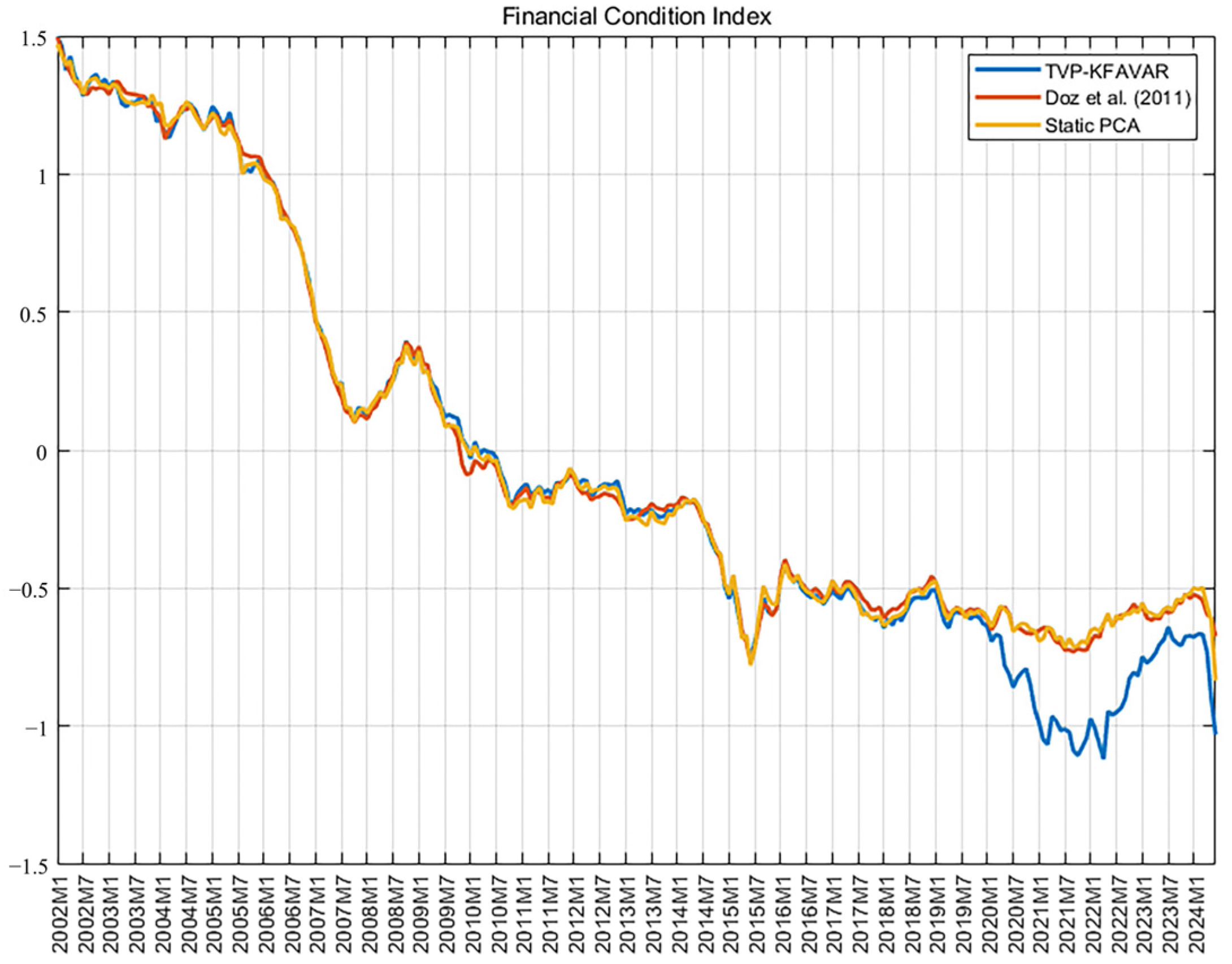
As shown in Figure 2, the blue line is the FCI calculated by the TVP-KFAVAR model, the yellow line is the FCI calculated by the Static PCA model, and the red line is the FCI calculated based on Doz et al. (2011) [49].

Scientific and practical Financial Conditions Index can effectively mirror a country’s financial stability during its historical period. A larger value of the Financial Conditions Index signifies better financial stability, whereas a smaller value indicates greater financial risk. By comparing the absolute value line chart of the Macro-Financial Conditions Index constructed herein (refer to Figure 2) with China’s actual circumstances, it becomes evident that the index can precisely reflect certain external shocks (such as the impact of the U.S. subprime mortgage crisis on China’s financial market in 2008, the Chinese stock market crash in 2015, and the influence of the COVID-19 pandemic in 2020).

4.2. Analysis of the Reasons for Changes in the FCI

The Financial Conditions Index (FCI) reflects the level of financial risk in China: a higher FCI indicates a more resilient financial system, while a lower value signifies greater financial risk. Compared with the FCI calculated by Doz et al. (2011) and the Static PCA model, the FCI derived from the TVP-KFAVAR model in this study exhibits more pronounced fluctuations between 2019 and 2023, enabling a more precise capture of financial risk levels during the pandemic [49]. Based on this, the study combines the Chinese Financial Conditions Index (FCI) calculated by the TVP-KFAVAR model (as shown in Figure 2) with historical events in China’s financial markets to analyze the reasons for FCI changes from 2002 to 2024.

4.2.1. 2008 Global Financial Crisis (FCI Decline)

The 2008 U.S. subprime mortgage crisis triggered a global financial meltdown, leading to a sharp decline in China’s exports, a stock market crash (the Shanghai Composite Index plunged from 6124 points to 1664 points), and tightened financial market liquidity. These factors exacerbated financial risks, potentially resulting in a relatively low Financial Conditions Index between July 2007 and January 2008.

4.2.2. 2009 “Four Trillion” Stimulus Plan (Financial Conditions Index Recovery)

In response to the crisis, the Chinese government implemented a CNY four trillion investment plan to inject liquidity and stimulate credit expansion. This policy revived the economy, stabilized the stock and real estate markets, and temporarily alleviated systemic risks. The Financial Conditions Index rebounded rapidly between July 2008 and January 2009, although subsequent data may reflect the accumulation of risks due to excessive credit growth.

4.2.3. 2015 Stock Market Turbulence (Financial Conditions Index Plummets)

From January 2015 to January 2016, China’s A-share market experienced a sharp decline after rapid growth, with thousands of stocks hitting their daily price limits, triggering widespread panic. This exposed the high financial leverage in China’s stock market and the vulnerabilities arising from market speculation. The FCI reached its relative lowest value in June 2015, coinciding with the peak of China’s A-share index, which then began to decline.

4.2.4. The Outbreak of the COVID-19 Pandemic in Early 2020 (The Financial Conditions Index Initially Fell and Then Rebounded)

The COVID-19 pandemic first emerged in early 2020, quickly triggering panic in the financial market and causing a sharp drop in Chinese stock market prices. Although the central bank’s proactive monetary easing and fiscal support helped stabilize the financial market, the FCI remained low and did not return to pre-pandemic levels until July 2023.

4.2.5. The A-Share Market Has Continued to Fall Since May 2024 (The Financial Conditions Index Has Taken a Sharp Turn for the Worse)

In early 2024, the manufacturing PMI remained below the boom–bust line for three consecutive months, and real estate investment fell by 8.2% year-on-year, dragging down upstream and downstream industrial chains (such as building materials and home appliances). Consumption recovery was weak, with retail sales growth slowing to 4.1%, residents’ savings propensity increased, and corporate earnings expectations were lowered, putting pressure on market valuations. Although the State Council issued the “28 Measures to Stabilize Growth” in March, the market was skeptical about the extent of real estate relaxation (for example, the funding rate for “guaranteed delivery of buildings” was only 65%) and the effectiveness of consumption stimulus (auto-subsidies were declining), with the policy transmission effect falling short of expectations. Following the implementation of new delisting rules in April 2024, the ST sector experienced a panic-driven decline. From May to September, a total of 112 companies were subjected to ST, with related stocks averaging a 45% decline, dragging down the performance of the small- and medium-cap index and causing the FCI to plummet rapidly.

Overall, the potential risks in China’s macro-financial market are elevated and exhibit a tendency to accumulate progressively over the years. Since 2015, the Chinese government has consistently emphasized the need to “prevent and resolve systemic financial risks” and has implemented a robust policy mix with the aim of curbing the further exacerbation of financial risks.

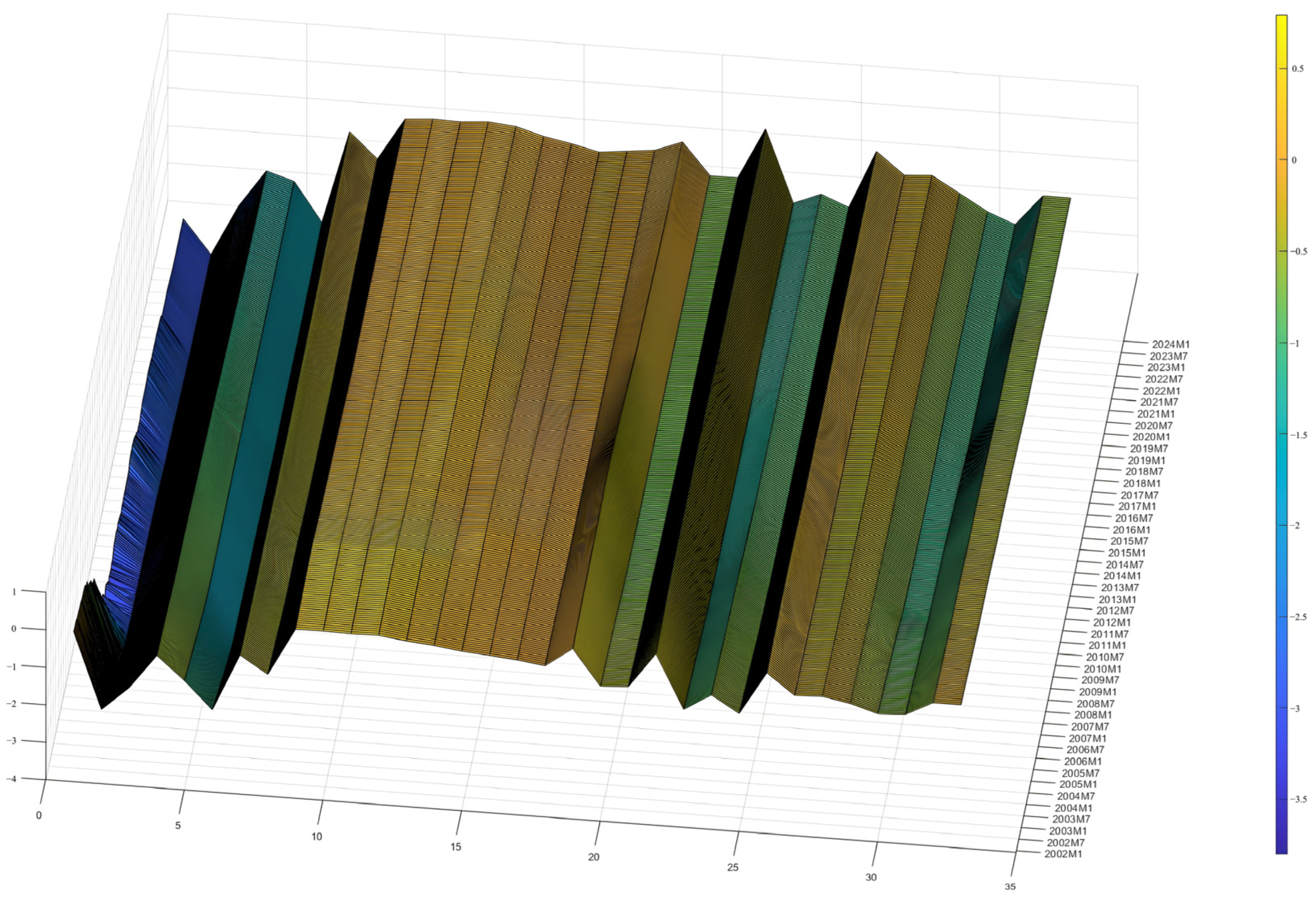
To more effectively achieve this objective, it is crucial to accurately gauge the true state of China’s financial risks. The TVP-KFAVAR model developed in this study employs kernel density PCA and time-varying factor loading coefficients to effectively capture the dynamic impact characteristics of each fundamental indicator on the Financial Conditions Index at various points in time.

As illustrated in Figure 3, all the basic indicators utilized in constructing the Financial Conditions Index exhibit distinct time-varying characteristics; lower factor loading curves correspond to stronger negative impacts on financial stability. Notably, stock market factors consistently occupy the lowest positions in the factor loading diagram, demonstrating their dominant role in influencing China’s financial stability.

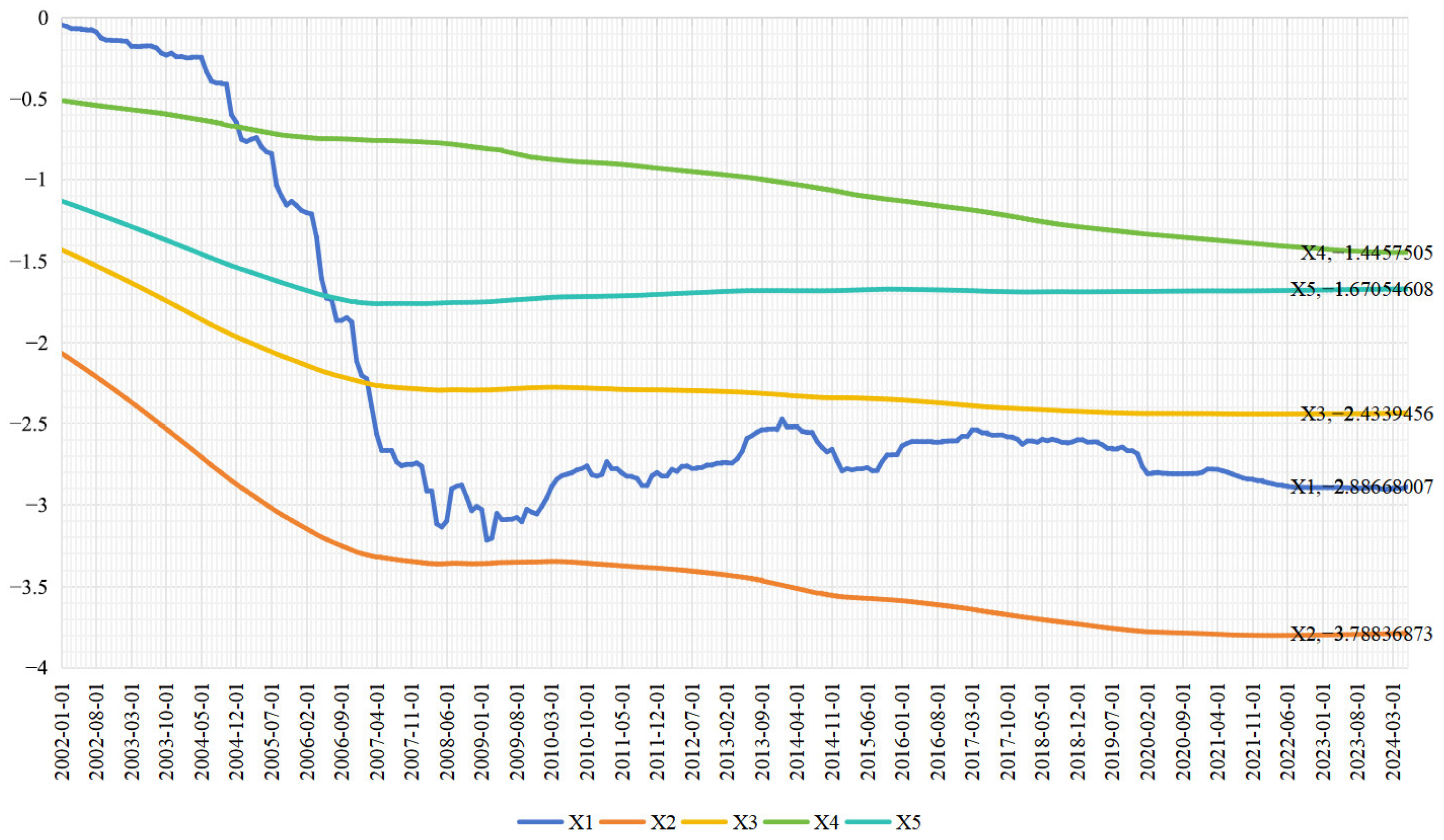
Upon closer examination of Figure 4, the Shanghai Composite Index (X2) exhibits a persistent downward trend, indicating its progressively stronger impact on financial stability over time. Meanwhile, the monthly closing price of the CSI 300 Index (X1) displays more volatile dynamics, with particularly sharp declines during two critical periods: the 2008 global financial crisis and the 2020 COVID-19 pandemic shock. These patterns clearly demonstrate the asymmetric nature of financial shocks.

The time-varying characteristics of factor loadings highlight the dynamic nature of financial factors’ impacts on China’s financial stability. These findings underscore the importance of monitoring the evolving relationships among financial indicators for effective financial risk management and policy formulation.

4.3. Plausibility Testing

To further assess the quality and applicability of the constructed “Macroeconomic Financial Conditions Index”, this study employs a multivariate vector autoregression (VAR) model to examine the predictive capacity of the Financial Conditions Index regarding relevant macroeconomic indicators.

Specifically, this paper employs the GDP growth rate, the natural logarithm of the national real estate boom index, and the natural logarithm of the macroeconomic boom index leading index to evaluate the predictive performance of the Financial Conditions Index (FCI).

(1) GDP Growth Rate: The GDP growth rate is the core indicator for measuring the expansion speed of a country’s total economic volume, reflecting the overall level of real economic activities. As a comprehensive proxy variable for financial conditions, the predictive ability of the FCI needs to be verified by its capacity to anticipate changes in the GDP growth rate. For instance, accommodative financial conditions can stimulate investment and consumption, thereby promoting GDP growth, while a restrictive financial environment may dampen economic activities. Selecting the GDP growth rate as the core variable allows for a direct test of the FCI’s predictive effectiveness regarding the overall macroeconomic volume.

(2) National Real Estate Prosperity Index: The real estate industry holds a “pillar” status in China’s economy, with its fluctuations exerting a broad impact on the macroeconomy through industrial chain transmission and financial intermediation. The National Real Estate Prosperity Index comprehensively reflects the cyclical fluctuations of key aspects such as real estate development investment, funding sources, and sales prices. Its leading characteristics provide an ideal framework for examining the transmission mechanism of FCI.

(3) Macroeconomic Prosperity Index-Leading Index: The Macroeconomic Prosperity Index-Leading Index is composed of a set of leading indicators (such as the PMI, consumer confidence index, production and sales ratio, etc.), designed to forecast the turning points of the economic cycle. Its leading properties are logically consistent with the forward-looking nature of FCI’s financial conditions: if FCI can influence this index in advance, it implies that the financial environment plays a guiding role in shaping the expectations of economic entities.

Prior to estimating the regression model, this study first conducted Augmented Dickey–Fuller (ADF) tests on the selected variables, including the constructed China Financial Conditions Index (FCI). The results, presented in

Table 2. ADF test results.

Variable	Difference Order	Test	p-Value
Financial Conditions Index	1	−2.925	0.0425
National Real Estate Prosperity Index	1	−2.956	0.0393
Macroeconomic Prosperity Index-Leading Index	0	−4.967	0.0000
GDP Growth Rate	0	−4.886	0.0000

, indicate that the GDP growth rate and the Macroeconomic Prosperity Index-Leading Index are stationary at the 1% significance level, confirming that their statistical properties remain stable over time without deterministic trends or unit roots.

In contrast, the National Real Estate Prosperity Index and the FCI exhibit non-stationarity in levels but achieve stationarity after first differencing at the 5% significance level. This suggests that these variables follow a unit root process (I(1))—meaning they are influenced by stochastic trends—and must be differenced to avoid spurious regression results.

Based on the VAR model estimation results presented in

Table 3. VAR model test.

L1.Financial Conditions Index	Coefficient	Std. Err.	p-Value
Financial Conditions Index	0.989	0.005	0.000
National Real Estate Prosperity Index	0.001	0.001	0.083
Macroeconomic Prosperity Index-Leading Index	0.003	0.001	0.000
GDP Growth Rate	0.005	0.001	0.000

, the first lag of the Financial Conditions Index (L1.FCI) exerts a significant positive influence on all the explanatory variables, as detailed below:

(1) The coefficient of the lagged term of FCI is 0.989 (p = 0.000), signifying that the Financial Conditions Index possesses a high degree of inertia, with its rising or falling state typically persisting for approximately one month.

(2) For each one-unit increase in FCI, the National Real Estate Boom Index rises by 0.001 (p = 0.083), a relationship that is statistically significant at the 10% confidence level. This finding reflects that enhancements in financial conditions can stimulate real estate demand via credit expansion.

(3) The coefficient of FCI on the Leading Index of the Macroeconomic Prosperity Index is 0.003 (p = 0.000), indicating that the Financial Conditions Index is capable of predicting the turning points of the economic cycle in advance.

(4) The coefficient of FCI on the GDP growth rate is 0.005 (p = 0.000), suggesting that improvements in financial conditions can exert a driving effect on the real economy through various channels, including investment and consumption.

In summary, the Financial Conditions Index (FCI) constructed in this paper is capable of accurately and effectively forecasting changes in macroeconomic variables, demonstrating a certain degree of applicability.

5. Further Discussion

In order to further explore the applicability of different prediction models to the assessment and early warning of China’s macro-financial conditions, this paper in this section performs time-series prediction of the FCI based on five types of mainstream deep learning algorithms, including LSTM, GRU, BiLSTM, TCN, and Transformer. The division ratio of training set and test set is 4:1. Meanwhile, we add ARIMA model as a benchmark for comparing the forecasting performance of deep learning algorithms and traditional time series analysis models for the FCI. The reasons for selecting the above deep learning algorithms in this paper are mainly due to the following: (1) FCI has an obvious nonlinear structure, which is not accurately portrayed by traditional time series models, and the above five deep learning algorithms are suitable for capturing this time series feature. (2) FCI is affected by many factors, and compared with traditional time series models, these five deep learning algorithms are good at dealing with more complex interactions among variables when considering high-dimensional inputs. (3) FCI belongs to the indicators with long period, strong inertia, and significant cumulative effect, and the above deep learning algorithms can capture the long-time dependency relationship to avoid the gradient disappearance and information attenuation, which is suitable to be used for FCI prediction.

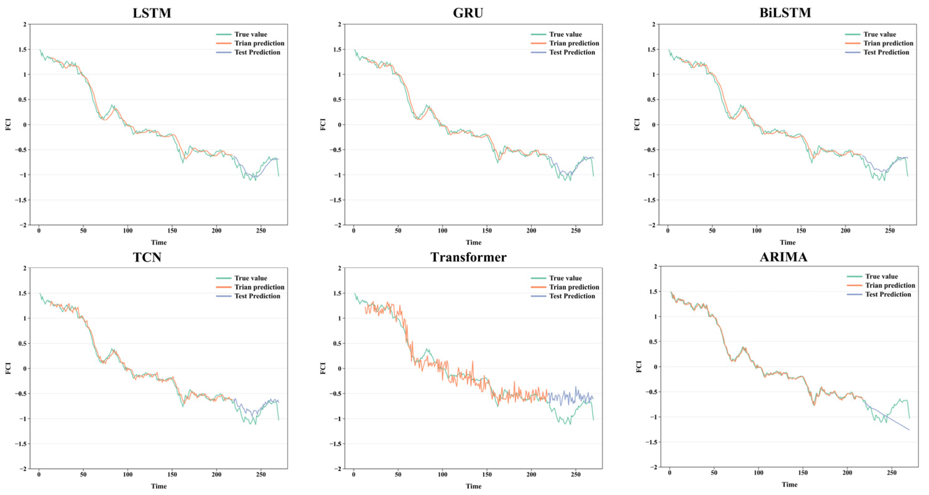
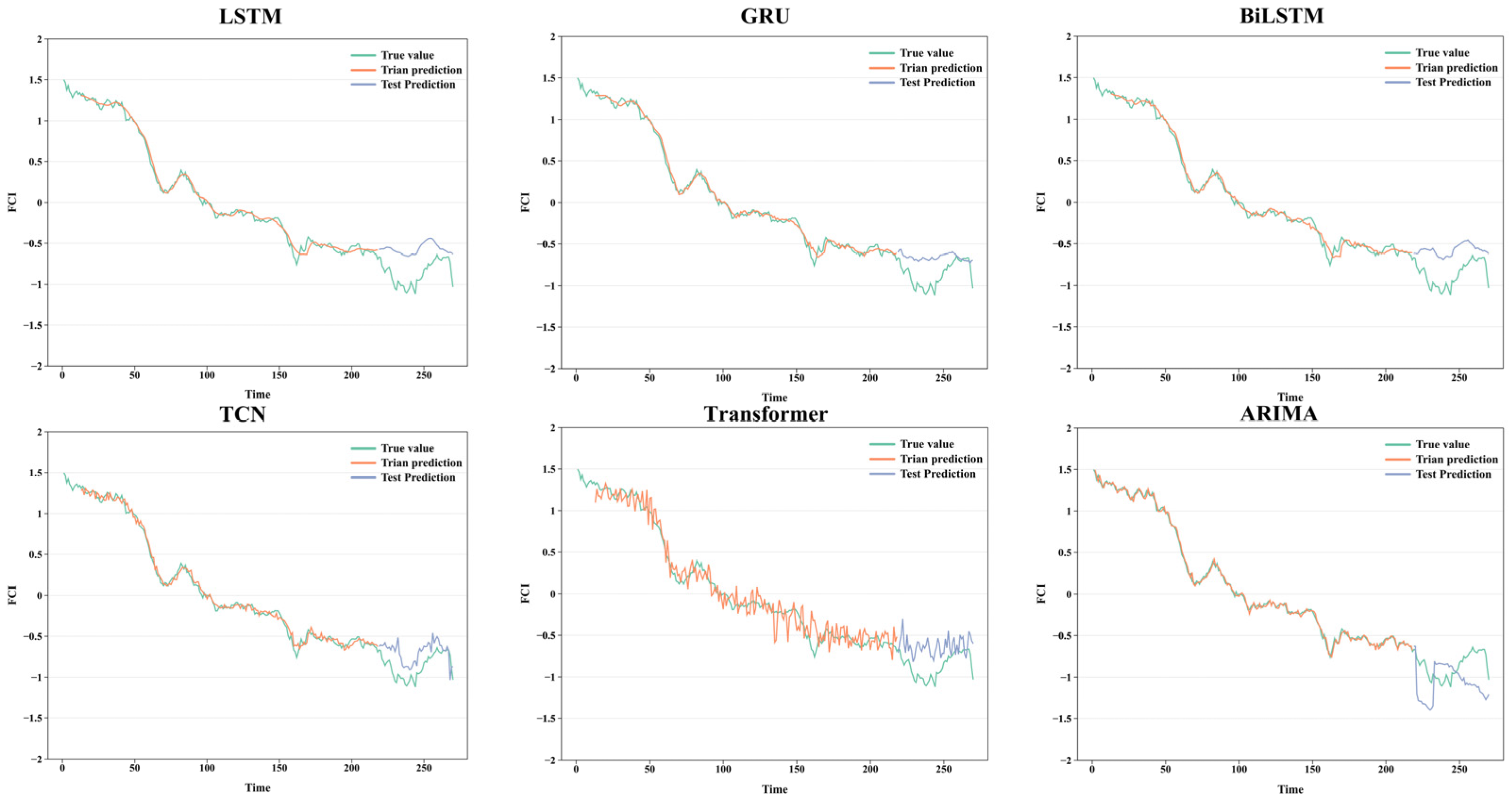
Figure 5 illustrates the univariate predictions of FCI by the six prediction models. It can be seen that the training fit of all models performs well, and the model predictions have a high degree of scientific validity and accuracy. Overall, the FCI predicted by the six models and the real value development of the trend are basically the same; the difference is small. This paper specifically evaluates the prediction performance of the models based on the root mean square error (RMSE), and the results are shown in

Table 4. Evaluation of univariate time series forecasting accuracy.

	LSTM	GRU	BiLSTM	TCN	Transformer	ARIMA
RMSE	0.1066	0.1045	0.1217	0.1446	0.3300	0.2853

.

When using only FCI as an input variable, the deep learning models outperform the ARIMA model in prediction, except for Transformer. The prediction accuracy of LSTM and its modified models (GRU, BiLSTM) is better among the five deep learning models. Among them, the GRU model has the highest prediction accuracy, with RMSE reaching 0.1066. The prediction performance of LSTM and BiLSTM ranked after GRU in that order. The prediction performance of the TCN model is second only to that of LSTM and its variants, with an RMSE of 0.1446, respectively. Transformer’s prediction accuracy for the FCI is not satisfactory and has the worst performance among all models.

Univariate variables provide very limited information for comparing the model’s prediction performance of the FCI with multivariate inputs. In addition to the FCI, this paper additionally selects 25 macroeconomic indicators in China and abroad as input variables to the model, specifically including CPI, GDP, ln(national housing prosperity index)/CPI, ln(social financing scale)/CPI, ln(gold reserves)/CPI, real estate development investment completion, provident fund interest rate of more than 5 years, ln(export amount of the month)/CPI, ln(import amount of the month)/CPI, ln(consumer confidence index)/CPI, ln(macroeconomic prosperity index − leading index)/CPI, ln(macroeconomic prosperity index − lagging index)/CPI, value added of industry above scale month-on-month, public finance revenue/CPI, public finance expenditure/CPI, S&P/CS house price index, CPI (US), m1 (US), m2 (US), federal funds rate, S&P500, Dow Jones, Nasdaq, S&P 500 returns, and ln(mGDP) (US). Figure 6 illustrates the trend in model forecasts with multivariate inputs. Since the traditional ARIMA model is unable to consider multivariate inputs, it is hereby replaced by the ARIMAX model, which can take into account exogenous influences.

According to Figure 6, it can be seen that the difference between the predicted trend and the actual trend of the FCI by most of the prediction models increased after considering more variables as inputs. Among them, the predictive performance of the LSTM, GRU, and BiLSTM models decreased most significantly.

Table 5. Evaluation of multivariate time series forecasting accuracy.

	LSTM	GRU	BiLSTM	TCN	Transformer	ARIMAX
RMSE	0.3180	0.2457	0.3110	0.2110	0.2803	0.3421

reports the prediction accuracy of the six models with multivariate inputs. All deep learning models are better at predicting FCI than the ARIMAX model. Except for the Transformer model, the prediction accuracies of all others decreased after considering multivariate inputs. Among them, the most significant decrease in accuracy is in the LSTM model, where the RMSE is reduced by 0.2114, respectively. TCN has the strongest prediction accuracy for the FCI under multivariate input conditions, and the prediction accuracies of the other models are, in descending order, GRU, Transformer, BiLSTM, LSTM, and ARIMAX.

In conclusion, traditional time-series models are significantly weaker than the vast majority of deep learning models in FCI prediction. The overall publication has a relatively good prediction performance of GRU for FCI, regardless of univariate or multivariate inputs. GRU has the highest prediction accuracy for FCI under univariate input conditions, while TCN performs optimally under multivariate input conditions.

This study corroborates the findings of Zhu et al. (2021) and Wang et al. (2024), confirming the significant time-varying characteristics of China’s Financial Conditions Index [12,28]. Methodologically, we demonstrate that traditional time-series analysis methods underperform machine learning models in FCI prediction—a critical gap overlooked in previous research. Through comprehensive evaluation of RMSE metrics and prediction curves, we reveal novel findings: the GRU model achieves optimal prediction performance under univariate input conditions, while the TCN model excels in multivariate scenarios. These results provide new methodological insights for financial condition forecasting. Future research could explore the integration of diverse machine learning models to identify the optimal model combinations for predicting China’s financial conditions across different economic environments.

6. Conclusions and Recommendations

6.1. Conclusions

This study proposes an innovative methodology for constructing China’s Macro-Financial Conditions Index to improve its explanatory power regarding financial conditions. Our findings demonstrate that (1) the TVP-KFAVAR-based FCI effectively captures the dynamic responses of China’s financial markets to both domestic and international shocks, (2) machine learning models exhibit significantly superior forecasting performance compared to traditional time-series methods. These results provide policymakers with enhanced analytical tools for financial monitoring. The key research conclusions are summarized as follows:

(1) Utilizing data from China’s financial market spanning the period from 2002 to 2024, this study selects 33 quantitative variables from the stock market, bond market, interest rate market, exchange rate market, derivative market, and money market to serve as the fundamental indicators of the Financial Conditions Index (FCI). Additionally, it incorporates 25 macroeconomic variables from both China and the United States as external response variables to construct the FCI. This comprehensive indicator system is capable of thoroughly evaluating China’s financial situation while also taking into account the external shock effects of the international market on China’s financial system. In contrast to previous studies, this research overcomes the limitation of neglecting the international market.

(2) Building upon the TVP-FAVAR model, this paper integrates the kernel density principal component analysis (PCA) model to develop an enhanced TVP-KFAVAR model. This enhancement allows the model to more effectively capture the nonlinearity and asymmetry that manifest during crises. Compared to traditional models, the TVP-KFAVAR model constructed in this study demonstrates superior recognition performance during the pandemic. Validation through the VAR model confirms that the improved FCI possesses significant predictive capabilities for the GDP growth rate, the national real estate prosperity index, and the leading index of the macroeconomic prosperity index.

(3) In further analysis, this paper employs ARIMA and its extended model and five machine learning algorithms to predict the FCI. It discovers that under single input conditions, the GRU model exhibits the best performance, with the TCN model being slightly less effective. Except for Transformer, all other machine learning algorithms outperformed the ARIMA model in terms of prediction accuracy. However, under multiple input conditions, the TCN model surpasses other models, followed by the GRU model. Both models significantly outperform the other algorithms. From the perspectives of fitting form and overall performance, the TCN model achieves the best prediction results, while ARIMAX, as a traditional time series model, has the worst prediction results.

6.2. Recommendations

(1) Based on the findings of this study, the methodology for constructing the FCI should be continuously refined. On one hand, it is recommended to regularly update and expand the underlying indicator system by incorporating more variables that reflect the dynamic characteristics of financial markets, such as emerging financial products and innovative financial instruments. On the other hand, the construction of the FCI must account for the complexity and volatility of international markets. To this end, it is advisable to enhance the monitoring and analysis of international macroeconomic variables, such as those from the Eurozone and Japan, thereby establishing a more robust response mechanism for global financial markets. Additionally, unconventional indicators like nighttime light remote sensing data could be considered for inclusion in the Macro-Financial Conditions Index framework. Such data, with their strong timeliness, can to some extent reflect economic activity and growth momentum, potentially serving as an effective factor in financial stability indices. By integrating these potential indicators, the comprehensiveness and forward-looking capability of the FCI can be further improved, ensuring its applicability and accuracy across diverse market conditions.

(2) Promote and apply the Time Series Variable-KFAVAR model. The research results show that the TVP-KFAVAR model has significant advantages in capturing the nonlinearity and asymmetry of the financial market, especially during crises. Therefore, this paper encourages policymakers and financial institutions to consider promoting and applying this improved model. At the same time, in the process of formulating financial risk management policies, full use should be made of the dynamic information and prediction results provided by the TVP-KFAVAR model to timely adjust and optimize financial regulatory policies, enhancing the stability and resilience of the financial system.

(3) Strengthen the application of machine learning algorithms in financial risk prediction. The research results indicate that both the GRU model and the TCN model perform well in FCI prediction, with the TCN model having the strongest comprehensive prediction ability under multi-input conditions. To further develop this field, it is recommended to strengthen the application of machine learning algorithms in financial risk prediction. Developing hybrid models that integrate multiple machine learning algorithms can leverage the advantages of each model, thereby improving the accuracy and stability of predictions. In addition, future research should consider strengthening the collection and processing of financial big data, utilizing advanced computing technologies to improve data processing efficiency, which will contribute to the scientific and reliable improvement of financial risk prediction.

References

1. Quan, Y.; Miao, W. Asymmetric Risk Contagion Effect of the Interaction between the Real Economy and the Financial Sector-an Analysis Based on the Domestic Commodity Price Index. Financ. Innov. 2025, 11, 55. [Google Scholar] [CrossRef]
2. Matheson, T.D. Financial Conditions Indexes for the United States and Euro Area. Econ. Lett. 2012, 115, 441–446. [Google Scholar] [CrossRef]
3. Koop, G.; Korobilis, D. A New Index of Financial Conditions. Eur. Econ. Rev. 2014, 71, 101–116. [Google Scholar] [CrossRef]
4. Debuque-Gonzales, M.; Socorro Gochoco-Bautista, M. Financial Conditions Indexes and Monetary Policy in Asia. Asian Econ. Pap. 2017, 16, 83–117. [Google Scholar] [CrossRef]
5. Armendariz, T.; Ramirez, C. Estimation of a Financial Conditions Index for Mexico. Trimest. Econ. 2017, 84, 899–946. [Google Scholar]
6. Wang, S.; Xu, F.; Chen, S. Constructing a Dynamic Financial Conditions Indexes by TVP-FAVAR Model. Appl. Econ. Lett. 2018, 25, 183–186. [Google Scholar] [CrossRef]
7. Giri, A.K.; Bansod, D. Establishing Finance-Growth Linkage for India: A Financial Conditions Index (FCI) Approach. IJOEM 2019, 14, 1032–1059. [Google Scholar] [CrossRef]
8. Osina, N. Global Liquidity, Market Sentiment, and Financial Stability Indices. J. Multinatl. Financ. Manag. 2019, 52–53, 100606. [Google Scholar] [CrossRef]
9. Chen, L.; Han, Q.; Qiao, Z.; Stanley, H.E. Correlation Analysis and Systemic Risk Measurement of Regional, Financial and Global Stock Indices. Phys. A Stat. Mech. Its Appl. 2020, 542, 122653. [Google Scholar] [CrossRef]
10. Carrillo, J.A.; Laura Garcia, A. The COVID-19 Economic Crisis in Mexico through the Lens of a Financial Conditions Index. Latin. Am. Econ. Rev. 2021, 30, 1–27. [Google Scholar] [CrossRef]
11. Tissaoui, K.; Hkiri, B.; Zaghdoudi, T.; Azibi, J. Illiquidity, Uncertainty Indices, and COVID-19 Outbreak Conditions: Empirical Evidence from the US Financial Market. Complexity 2022, 2022, 2818633. [Google Scholar] [CrossRef]
12. Zhu, S.; Kavanagh, E.; O’Sullivan, N. Constructing a Financial Conditions Index for the United Kingdom: A Comparative Analysis. Int. J. Financ. Econ. 2021, 26, 2976–2989. [Google Scholar] [CrossRef]
13. Ferriani, F.; Gazzani, A. Financial Condition Indices for Emerging Market Economies: Can Google Help? Econ. Lett. 2022, 216, 110528. [Google Scholar] [CrossRef]
14. Deng, Y.; Zhang, Z.; Zhu, L. A Model-Based Index for Systemic Risk Contribution Measurement in Financial Networks. Econ. Model. 2021, 95, 35–48. [Google Scholar] [CrossRef]
15. Chabot, M. Financial Stability Indices and Financial Networks Dynamics in Europe. Rev. Econ. 2021, 72, 591–631. [Google Scholar] [CrossRef]
16. AL-Rjoub, S.A.M. A Financial Stability Index for Jordan. J. Cent. Bank Theor. Pract. 2021, 10, 157–178. [Google Scholar] [CrossRef]
17. Gustiana, A. Nasrudin Evaluating Financial System Stability Using Heatmap from Aggregate Financial Stability Index with Change Point Analysis Approach. Asia-Pac. Financ. Mark. 2021, 28, 367–396. [Google Scholar] [CrossRef]
18. Kabundi, A.; Mbelu, A. Estimating a Time-Varying Financial Conditions Index for South Africa. Empir Econ. 2021, 60, 1817–1844. [Google Scholar] [CrossRef]
19. Chiappari, M.; Scotti, F.; Flori, A. Hedging Financial Risks with a Climate Index Based on EU ETS Firms. Energy 2025, 320, 135277. [Google Scholar] [CrossRef]
20. Ganchev, G.T.; Paskaleva, M.G. The Importance of Financial Condition Indices in South-Eastern Europe. Int. J. Contemp. Econ. Adm. Sci. 2020, 10, 78–106. [Google Scholar] [CrossRef]
21. Brum-Civelli, C.; Fried-Gindel, A.; Garcia-Hiernaux, A. IFCI-SA: International Financial Conditions Index for South American Economies. Res. Int. Bus. Financ. 2024, 72, 102507. [Google Scholar] [CrossRef]
22. Bas, T.; Malki, I.; Sivaprasad, S. Connectedness between Central Bank Digital Currency Index, Financial Stability and Digital Assets. J. Int. Financ. Mark. Inst. Money 2024, 92, 101981. [Google Scholar] [CrossRef]
23. Zhang, W. Dynamic Monitoring of Financial Security Risks: A Novel China Financial Risk Index and an Early Warning System. Econ. Lett. 2024, 234, 111445. [Google Scholar] [CrossRef]
24. Kazdal, A.; Korkmaz, H.I.; Yilmaz, M.H. Composing a High-Frequency Financial Conditions Index and the Implications for Economic Activity. Borsa Istanb. Rev. 2022, 22, 769–779. [Google Scholar] [CrossRef]
25. Morana, C. A New Macro-Financial Condition Index for the Euro Area. Econom. Stat. 2024, 29, 64–87. [Google Scholar] [CrossRef]
26. Sahoo, J. Financial Stress Index, Growth and Price Stability in India: Some Recent Evidence. Transnatl. Corp. Rev. 2021, 13, 222–236. [Google Scholar] [CrossRef]
27. Angelopoulou, E.; Balfoussia, H.; Gibson, H.D. Building a Financial Conditions Index for the Euro Area and Selected Euro Area Countries: What Does It Tell Us about the Crisis? Econ. Model. 2014, 38, 392–403. [Google Scholar] [CrossRef]
28. Wang, J.; Tang, W. Construction and Analysis of Chinese Macro-Financial Stability Index. Comput Econ. 2024. [Google Scholar] [CrossRef]
29. Lupu, R.; Călin, A.C.; Dumitrescu, D.G.; Lupu, I. Introducing a Novel Fragility Index for Assessing Financial Stability amid Asset Bubble Episodes. N. Am. J. Econ. Financ. 2025, 75, 102291. [Google Scholar] [CrossRef]
30. Reynolds, S.; Fowles, R.; Gander, J.; Kunaporntham, W.; Ratanakomut, S. Forecasting the Probability of Failure of Thailand’s Financial Companies in the Asian Financial Crisis. Econ. Dev. Cult. Change 2002, 51, 237–246. [Google Scholar] [CrossRef]
31. Niemira, M.P.; Saaty, T.L. An Analytic Network Process Model for Financial-Crisis Forecasting. Int. J. Forecast. 2004, 20, 573–587. [Google Scholar] [CrossRef]
32. Chang, J.; Cho, Y.J.; Shin, H.-H. The Change in Corporate Transparency of Korean Firms after the Asian Financial Crisis: An Analysis Using Analysts’ Forecast Data. Corp. Gov. 2007, 15, 1144–1167. [Google Scholar] [CrossRef]
33. Yu, L.; Wang, S.; Lai, K.K.; Wen, F. A Multiscale Neural Network Learning Paradigm for Financial Crisis Forecasting. Neurocomputing 2010, 73, 716–725. [Google Scholar] [CrossRef]
34. Zaleskiewicz, T. Financial Forecasts during the Crisis: Were Experts More Accurate than Laypeople? J. Econ. Psychol. 2011, 32, 384–390. [Google Scholar] [CrossRef]
35. Halbleib, R.; Pohlmeier, W. Improving the Value at Risk Forecasts: Theory and Evidence from the Financial Crisis. J. Econ. Dyn. Control 2012, 36, 1212–1228. [Google Scholar] [CrossRef]
36. Chen, C.W.S.; Gerlach, R.; Lin, E.M.H.; Lee, W.C.W. Bayesian Forecasting for Financial Risk Management, Pre and Post the Global Financial Crisis. J. Forecast. 2012, 31, 661–687. [Google Scholar] [CrossRef]
37. Metescu, A.-M.; Borisov, D.; Banica, R.M. Forecasting Rates of Return Using Geometric Brownian Motion during the Global Financial Crisis Period. Metal. Int. 2013, 18, 134–137. [Google Scholar]
38. Berger, T.; Missong, M. Financial Crisis, Value-at-Risk Forecasts and the Puzzle of Dependency Modeling. Int. Rev. Financ. Anal. 2014, 33, 33–38. [Google Scholar] [CrossRef]
39. Audrino, F. Forecasting Correlations during the Late-2000s Financial Crisis: The Short-Run Component, the Long-Run Component, and Structural Breaks. Comput. Stat. Data Anal. 2014, 76, 43–60. [Google Scholar] [CrossRef]
40. Alessi, L.; Ghysels, E.; Onorante, L.; Peach, R.; Potter, S. Central Bank Macroeconomic Forecasting during the Global Financial Crisis: The European Central Bank and Federal Reserve Bank of New York Experiences. J. Bus. Econ. Stat. 2014, 32, 483–500. [Google Scholar] [CrossRef]
41. Kunze, F.; Kramer, J.; Rudschuck, N. Interest Rate Forecasts in Times of Financial Crisis: What Might Be Interesting to Know? Eur. J. Polit. Econ. 2014, 34, S45–S52. [Google Scholar] [CrossRef]
42. Cao, W.; Cao, L. Financial Crisis Forecasting via Coupled Market State Analysis. IEEE Intell. Syst. 2015, 30, 18–25. [Google Scholar] [CrossRef]
43. Makoni, T.; Chikobvu, D. Assessing and Forecasting the Long-Term Impact of the Global Financial Crisis on Manufacturing Sales in South Africa. Economies 2023, 11, 158. [Google Scholar] [CrossRef]
44. Colladon, A.F.; Grassi, S.; Ravazzolo, F.; Violante, F. Forecasting Financial Markets with Semantic Network Analysis in the COVID-19 Crisis. J. Forecast. 2023, 42, 1187–1204. [Google Scholar] [CrossRef]
45. Abrego-Perez, A.L.; Pacheco-Carvajal, N.; Diaz-Jimenez, M.C. Forecasting Agricultural Financial Weather Risk Using PCA and SSA in an Index Insurance Model in Low-Income Economies. Appl. Sci. 2023, 13, 2425. [Google Scholar] [CrossRef]
46. Li, Y.; Liang, C.; Huynh, T.L.D. Combination Forecast Based on Financial Stress Categories for Global Equity Market Volatility: The Evidence during the COVID-19 and the Global Financial Crisis Periods. Appl. Econ. 2024, 56, 4435–4470. [Google Scholar] [CrossRef]
47. Hafiz, F.; Broekaert, J.; Swain, A. Evolution of Neural Architectures for Financial Forecasting: A Note on Data Incompatibility during Crisis Periods. Ann. Oper. Res. 2024, 346, 1011–1025. [Google Scholar] [CrossRef]
48. Koong, S.S.; Law, S.H.; Ibrahim, M.H. Credit Expansion and Financial Stability in Malaysia. Econ. Model. 2017, 61, 339–350. [Google Scholar] [CrossRef]
49. Doz, C.; Giannone, D.; Reichlin, L. A Two-Step Estimator for Large Approximate Dynamic Factor Models Based on Kalman Filtering. J. Econom. 2011, 164, 188–205. [Google Scholar] [CrossRef]
Figure 1. LSTM cell diagram.
Symmetry 17 00904 g001
Figure 2. Financial Conditions Index [49].
Symmetry 17 00904 g002
Figure 3. Factor loadings. In the figure, color intensity represents the magnitude of factor loadings. Bluer shades indicate lower factor loadings, while yellower shades indicate higher factor loadings.
Symmetry 17 00904 g003
Figure 4. Stock market factor coefficients.
Symmetry 17 00904 g004
Figure 5. Univariate time series forecasting.
Symmetry 17 00904 g005
Figure 6. Multivariate time series forecasting.
Symmetry 17 00904 g006