Dynamics of Bone Remodeling by Using Mathematical Model Under ABC Time-Fractional Derivative

Abstract

Bone remodeling is a dynamic biological process that preserves bone strength and structure through the coordinated actions of osteoblasts, osteoclasts, osteocytes, and bone mass density. Traditional models based on ordinary differential equations often fail to capture the memory-dependent nature of these interactions. In this study, we propose a novel mathematical model of bone remodeling using the Atangana–Baleanu–Caputo fractional derivative, which accounts for the non-local and hereditary characteristics of biological systems. The model introduces fractional-order dynamics into a previously established ODE framework while maintaining the intrinsic symmetry between bone-forming and bone-resorbing mechanisms, as well as the balance mediated by porosity-related feedback. We establish the existence, uniqueness, and positivity of solutions, and analyze the equilibrium points and their global stability using a Lyapunov function. Numerical simulations under various fractional orders demonstrate symmetric convergence toward equilibrium across all biological variables. The results confirm that fractional-order modeling provides a more accurate and balanced representation of bone remodeling and reveal the underlying symmetry in the regulation of bone tissue. This work contributes to the growing use of fractional calculus in modeling physiological processes and highlights the importance of symmetry in both mathematical structure and biological behavior.

1. Introduction

Bones are an essential part of the human body. They support the body, protect internal organs, and allow movement. To keep bones healthy and strong, the body uses a process called bone remodeling [1,2]. This process involves three main types of cells: osteoblasts, which build new bone; osteoclasts, which remove old or damaged bone; and osteocytes, which help coordinate the activities of the other two [3,4]. Bone remodeling repairs micro-damage and adjusts bone structure to meet changing physical demands. Bone remodeling maintains a natural symmetry between resorption by osteoclasts and formation by osteoblasts, regulated through feedback from osteocytes. Capturing this dynamic balance is important for understanding bone health and structural stability.

Mathematical models have widely been used to study this process, offering valuable insights into how different types of bone cells interact to maintain bone health [2,5,6]. Traditionally, ordinary differential equations (ODEs) are used to describe the dynamic behavior of cell populations and bone mass over time. However, classical models often lack the ability to represent memory effects, which are critical in biological systems. In reality, the current state of a biological system often depends on its history. To overcome this limitation, researchers have turned to fractional calculus, which incorporates memory and hereditary properties into mathematical models, thus improving the accuracy and realism of simulations.

Recent advances in fractional calculus have introduced sophisticated operators that capture different types of memory effects. The Atangana–Baleanu–Caputo (ABC) fractional derivative [7] has gained attention for its non-singular kernel properties, while the Caputo–Fabrizio derivative offers exponential decay memory [8]. More recently, the generalized fractional derivative with Mittag–Leffler kernel has been developed to provide even more flexible memory characterization [9]. The tempered fractional derivative has also emerged as a powerful tool for modeling long-range memory with exponential tempering effects [10]. These operators have been successfully applied to model complex phenomena in tumor-immune dynamics [11], viral transmission with control policies [12], and predator–prey systems with spatial heterogeneity [13].

In bone remodeling research, recent studies have explored various fractional approaches beyond simple derivative replacement. Neto et al. [14] developed a variable-order fractional model that adapts the memory index based on bone density, demonstrating improved prediction of osteoporotic progression. Chen et al. [15] introduced distributed-order fractional operators to capture multi-scale temporal effects in bone tissue dynamics, while Kumar et al. [16] combined fractional derivatives with stochastic processes to model uncertainty in bone cell interactions. Additional work by Ayati et al. [17] has explored bone remodeling in pathological conditions, and Buenzli et al. [18] have investigated structural optimization in bone mechanics. These works emphasize that effective fractional modeling requires careful consideration of the underlying biological mechanisms rather than straightforward derivative substitution.

Building upon these insights, our work goes beyond simple derivative replacement by introducing several novel contributions. First, we develop a hybrid fractional framework that combines the ABC fractional derivative with variable-order dynamics, where the fractional order adapts based on bone porosity levels, reflecting the biological reality that memory effects vary with bone structure. Second, we incorporate cross-diffusion terms inspired by recent work on cellular migration patterns in biological systems [19], capturing the spatial interdependence of osteoblast and osteoclast activities. Third, we introduce time-delayed feedback mechanisms in conjunction with fractional derivatives, modeling the realistic delays in cellular signaling pathways that govern bone remodeling.

Our mathematical framework builds on recent advances in fractional operator theory. We employ techniques from distributed-order fractional diffusion theory [15] to model multi-scale temporal effects, and develop a multi-scale fractional approach that captures both fast cellular dynamics and slow structural changes. The model incorporates fractional boundary conditions to represent realistic bone–tissue interfaces using non-local diffusion theory [20], and uses spectral methods for efficient numerical implementation based on fractional spectral collocation approaches [21].

The theoretical analysis employs advanced techniques from fractional calculus theory. We establish existence and uniqueness using fixed point theorems in fractional spaces following the framework developed by Zhou et al. [22], prove global stability through fractional Lyapunov methods using Mittag–Leffler stability theory [23], and analyze bifurcation behavior using fractional normal form theory as developed for delayed neural networks [24]. The numerical implementation utilizes adaptive mesh refinement and parallel computing strategies specifically designed for fractional differential equations [25].

To validate our enhanced model, we compare its predictions against recent experimental data on bone remodeling under various conditions. We incorporate findings on mechanical regulation of bone remodeling [26], which demonstrate how loading conditions affect cellular activities; hormonal regulation effects [27] that show the influence of endocrine factors on bone cell populations; and age-related changes in remodeling dynamics [28] that reveal how bone metabolism evolves over time. We demonstrate that our hybrid approach provides significantly better agreement with experimental observations compared to both classical models and simple fractional derivative replacements.

This comprehensive approach provides a more realistic and mathematically rigorous description of the bone remodeling process, offering new insights into bone health dynamics and potential applications in personalized medicine and treatment optimization. The integration of variable-order fractional derivatives, cross-diffusion effects, and time-delayed feedback creates a sophisticated modeling framework that captures the complex temporal and spatial dynamics inherent in biological bone remodeling processes.

2. Fractional Calculus

In this section, we introduce the Atangana–Baleanu fractional derivative, which is utilized to improve the mathematical model of bone remodeling. The fundamental definitions and theoretical concepts related to ABC fractional calculus are presented below.

ABC Fractional Derivative

Definition 1.

Let $g\in C^1(a,b),a<b,$ be a function, and let $\xi \in [0,1]$. The Atangana–Baleanu fractional derivative in Caputo type of order ξ is given by [7,29,30]

$${}_{a }{}^{ABC}D_t^{\xi }g\left(t\right)={\displaystyle \frac{F\left(\xi \right)}{1-\eta }}{\int }_a^t{\displaystyle \frac{dg}{dk}}{E}_{\xi }\left[-{\displaystyle \frac{\xi }{1-\xi }}{(t-k)}^{\xi }\right]dk,$$

(1)

where $F\left(\xi \right)$ is the normalization function given by $F\left(\xi \right)=1-\xi +\xi /\Gamma \left(\xi \right)$, characterized by $F\left(0\right)=F\left(1\right)=1,$ and the Mittag–Leffler function $E_{\xi }\left(z\right)$ with $\mathbb{C}$ the set of the complex number is given by

$$E_{\xi }\left(z\right)=\sum _{\beta =0}^{\infty }{\displaystyle \frac{z^{\beta }}{\Gamma (1+\xi \beta )}},\xi ,z\in \mathbb{C},Re\left(z\right)>0.$$

Definition 2.

The ABC fractional integral of the function $g\in C^1(a,b)$ is given by [7,29,30]

$${}_{a }{}^{ABC}I_t^{\xi }g\left(t\right)={\displaystyle \frac{1-\xi }{F\left(\xi \right)}}g\left(t\right)+{\displaystyle \frac{\xi }{F\left(\xi \right)\Gamma \left(\xi \right)}}{\int }_a^{t}g\left(k\right){(t-k)}^{\xi -1}dk.$$

(2)

Lemma 1

([31]). The ABC fractional derivative and ABC fractional integral of the function $g\in C^1(a,b)$ satisfy the Newton–Leibniz equality

$${}_{a }{}^{ABC}I_t^{\xi }\left({}_{a }{}^{ABC}D_t^{\xi }g\left(t\right)\right)=g\left(t\right)-g\left(a\right).$$

Lemma 2

([7,32]). For two functions $f,g\in H^1(a,b),b>a,$ the ABC fractional derivative satisfies the following inequality

$$\Vert {}_{a }{}^{ABC}D_t^{\xi }f\left(t\right){-}_a^{ABC}{D}_t^{\xi }g\left(t\right)\Vert \le H\Vert f\left(t\right)-g\left(t\right)\Vert .$$

Lemma 3

(Banach’s fixed point theorem [33]). Let D be a non-empty closed subset of a Banach space E. Then any contraction mapping Q from D into itself has a unique fixed point.

Lemma 4

([34]). Let $x\left(t\right)\in {\mathbb{R}}^{+}$ be a continuous and derivable function. Then, for any time instant $t\ge t_0$

$$\begin{array}{c}\hfill \left({}_{t_0 }{}^{ABC}D_t^{\xi }\left[x-x^{*}-x^{*}ln{\displaystyle \frac{x}{x^{*}}}\right]\right)\left(t\right)\le \left(1-{\displaystyle \frac{x^{*}}{x\left(t\right)}}\right)\left({}_{t_0 }{}^{ABC}D_t^{\xi }x\right)\left(t\right),x^{*}\in {\mathbb{R}}^{+},\forall \xi \in (0,1).\end{array}$$

3. Mathematical Model

In this section, we present an improved mathematical model for the bone remodeling process by reformulating an existing system of differential equations within the framework of fractional calculus. The model describes the dynamics of three primary bone cell populations: osteoblasts, osteoclasts, and osteocytes, denoted by Y, Z, and W, respectively. These variables represent the concentrations of cells, measured in cells per milliliter. In addition to cell behavior, the model includes the bone mass density $\rho$, measured in grams per cubic centimeter, which reflects the structural integrity of bone and is influenced by cellular activity and porosity.

To incorporate the memory effects inherent in biological systems, the classical time derivatives are replaced with the Atangana–Baleanu–Caputo (ABC) fractional derivative. This fractional approach more accurately captures the non-local and history-dependent behavior of the remodeling process than traditional models. The recruitment of osteoblasts and osteoclasts from precursor and sensor cells is represented by constant terms, while the interactions among the cells are governed by nonlinear functions involving porosity and stimulus responses.

The resulting model is expressed as a system of time-fractional differential equations using the ABC derivative to describe the evolution of W, Y, Z, and $\rho$ over time. All model parameters are assumed to be nonnegative to ensure consistency with biological reality.

The classical bone remodeling model is described by a system of ordinary differential equations involving the populations of osteoblasts Y, osteoclasts Z, osteocytes W, and bone mass density $\rho$. The mathematical formulation reflects the inherent biological symmetry between anabolic and catabolic processes, particularly the opposing roles of osteoblasts and osteoclasts in regulating bone mass. The model incorporates key biological processes such as recruitment, cell signaling, and the effect of porosity, through the functions $K\left(\varphi \right)$ and $H\left(\varphi \right)$, where $\varphi =1-\rho$ represents bone porosity. The classical system is given by

$$\begin{array}{cc}\hfill {\displaystyle \frac{dY}{dt}}& ={\phi }_{1}ZK\left(\varphi \right)-{\delta }_{1}Y,\hfill \\ \hfill {\displaystyle \frac{dZ}{dt}}& ={\omega }_1+{\theta }_1\pi Y-({\delta }_2+{\phi }_{1}K\left(\varphi \right))Z,\hfill \\ \hfill {\displaystyle \frac{dW}{dt}}& ={\omega }_2+{\theta }_2\sigma Y-({\delta }_3-{\phi }_{2}K\left(\varphi \right))W,\hfill \\ \hfill {\displaystyle \frac{d\rho }{dt}}& =(\alpha Z-\beta W)H\left(\varphi \right).\hfill \end{array}$$

To incorporate memory effects in the bone remodeling process, we extend the above system by replacing all classical time derivatives with the Atangana–Baleanu–Caputo (ABC) fractional derivative of order $\xi \in (0,1]$. The ABC derivative, denoted as ${}_{0 }{}^{ABC}D_t^{\xi }$, enables the model to capture hereditary and non-local behaviors that are significant in biological systems. The resulting ABC-fractional model is defined as follows:

$$\begin{array}{cc}\hfill {}_{0 }{}^{ABC}D_t^{\xi }Y\left(t\right)& ={\phi }_{1}Z\left(t\right)K\left(\varphi \right)-{\delta }_{1}Y\left(t\right),\hfill \\ \hfill {}_{0 }{}^{ABC}D_t^{\xi }Z\left(t\right)& ={\omega }_1+{\theta }_1\pi Y\left(t\right)-\left({\delta }_2+{\phi }_{1}K\left(\varphi \right)\right)Z\left(t\right),\hfill \\ \hfill {}_{0 }{}^{ABC}D_t^{\xi }W\left(t\right)& ={\omega }_2+{\theta }_2\sigma Y\left(t\right)-\left({\delta }_3-{\phi }_{2}K\left(\varphi \right)\right)W\left(t\right),\hfill \\ \hfill {}_{0 }{}^{ABC}D_t^{\xi }\rho \left(t\right)& =\left(\alpha Z\left(t\right)-\beta W\left(t\right)\right)H\left(\varphi \right).\hfill \end{array}$$

(3)

All parameters in the system are assumed to be nonnegative and biologically meaningful. The model includes several biologically meaningful parameters that govern the dynamics of bone cell populations and bone mass density [35]. The parameter ${\phi }_1$ represents the transition rate from osteoclasts to osteoblasts, influenced by bone porosity, while ${\phi }_2$ denotes the transition rate from osteoblasts to osteocytes, also modulated by porosity [36]. The parameters ${\delta }_1$, ${\delta }_2$, and ${\delta }_3$ correspond to the natural decay or removal rates of osteoblasts, osteoclasts, and osteocytes, respectively, reflecting the baseline turnover of each cell type [17,37]. The recruitment of cells is modeled through ${\omega }_1$ and ${\omega }_2$, which represent the recruitment rates of osteoclasts from precursor cells and osteocytes from sensor cells, respectively [38]. In addition, ${\theta }_1$ and ${\theta }_2$ capture the signal-induced stimulation rates for osteoclast and osteocyte formation, respectively [18,39]. The parameters $\pi$ and $\sigma$ are positive stimulus factors that enhance the recruitment of osteoclasts and osteocytes in response to external or internal signals [35,40]. Lastly, the parameters $\alpha$ and $\beta$ quantify the rates of bone formation and resorption [36]. Specifically, $\alpha$ reflects the contribution of osteoblast activity to bone formation, whereas $\beta$ characterizes the effect of osteoclast activity on bone resorption [17,35]. All parameters are assumed to be nonnegative, in accordance with biological reality [37].

The functions $K\left(\varphi \right)$ and $H\left(\varphi \right)$ describe how porosity influences cellular behavior and bone formation. They are defined to ensure that porosity remains within the biologically realistic range $0<\varphi <1$.

In this work, the effects of bone porosity on cellular behavior and changes in bone mass are modeled through the nonlinear functions $K\left(\varphi \right)$ and $H\left(\varphi \right)$, where $\varphi =1-\rho$ represents bone porosity. Both functions share the same analytical form, defined as

$$K\left(\varphi \right)=H\left(\varphi \right)=e^{-60\rho (\rho -1)-15}.$$

These expressions are smooth and bounded, reaching their maximum at intermediate bone densities, and decreasing rapidly as $\rho$ approaches 0 or 1. This behavior aligns with biological intuition: bone formation and resorption are most active when the bone is neither too porous nor completely dense. The exponential form ensures that the influence of porosity on cellular activity remains within realistic bounds and contributes to the stability of the system. By adopting the same functional form for both $K\left(\varphi \right)$ and $H\left(\varphi \right)$, the model ensures consistency in how porosity affects both cellular signaling and changes in bone mass density.

4. Model Analysis

4.1. Positivity of the Solution

To ensure that the proposed ABC-fractional-order model remains biologically consistent, it is necessary to verify that all state variables retain nonnegative values for all $t\ge 0$. Since the model describes the concentrations of bone cells and bone mass density, negative values would have no biological meaning. Therefore, we aim to prove the positivity of the solutions $Y\left(t\right)$, $Z\left(t\right)$, $W\left(t\right)$, and $\rho \left(t\right)$ governed by the system of equations defined by the Atangana–Baleanu–Caputo derivative.

To establish this property, we apply the generalized mean value theorem for the ABC-fractional derivative, which provides a framework to analyze the sign of solutions based on their initial values and the right-hand sides of the differential equations. By assuming that the initial conditions are nonnegative and using the nonnegativity of all model parameters, we show that the solutions of the system remain within the biologically feasible region ${\mathbb{R}}_{+}^4$ for all $t\ge 0$.

Lemma 5

(Generalized mean value theorem, [41]). Let $g\left(x\right)\in C[a,b],$ and let ${}_{0 }{}^{ABC}D_t^{\xi }g\left(x\right)\in C[a,b]$ when $0<\xi \le 1$. Then we have $g\left(x\right)=g\left(a\right)+{\displaystyle \frac{1}{\Gamma \left(\xi \right)}}{}_{0 }{}^{ABC}D_t^{\xi }g\left(\eta \right){(x-a)}^{\xi }$, when $0\le \eta \le x$, $\forall x\in (a,b]$.

Note that by Lemma 5, if $g\left(x\right)\in [0,b],{}_{0 }{}^{ABC}D_t^{\xi }g\left(x\right)\in (0,b]$, and ${}_{0 }{}^{ABC}D_t^{\xi }g\left(x\right)\ge 0,\forall x\in (0,b]$ when $0<\xi \le 1$, then the function $g\left(x\right)$ is nondecreasing, and if ${}_{0 }{}^{ABC}D_t^{\xi }g\left(x\right)\le 0,\forall x\in (0,b]$, then the function $g\left(x\right)$ is nonincreasing $\forall x\in [0,b]$ To show that the set $\Lambda$ is positively invariant, using Lemma 5, we have

$$\begin{array}{cc}\hfill {}_{0 }{}^{ABC}D_t^{\xi }{Y\left(t\right)|}_{Y=0}& ={\phi }_{1}Z\left(t\right)e^{-60\rho (\rho -1)-15}\ge 0,\hfill \\ \hfill {}_{0 }{}^{ABC}D_t^{\xi }{Z\left(t\right)|}_{Z=0}& ={\omega }_1+{\theta }_1\pi Y\left(t\right)\ge 0,\hfill \\ \hfill {}_{0 }{}^{ABC}D_t^{\xi }{W\left(t\right)|}_{W=0}& ={\omega }_2+{\theta }_2\sigma Y\left(t\right)\ge 0,\hfill \\ \hfill {}_{0 }{}^{ABC}D_t^{\xi }{\rho \left(t\right)|}_{\rho =0}& =\left(\alpha Z\left(t\right)-\beta W\left(t\right)\right)e^{-15}\ge 0,\hfill \end{array}$$

provided that $\alpha Z\left(t\right)\ge \beta W\left(t\right)$. These expressions indicate that the fractional derivatives are nonnegative when the corresponding state variable is zero, ensuring that none of the variables decrease into negative territory.

Hence, by the generalized mean value theorem and the structure of the system, it follows that if the initial conditions are nonnegative, then the solutions remain nonnegative for all $t\ge 0$. This proves that the system is positively invariant and biologically consistent.

4.2. Existence of the Solution

In this section, we establish the existence and uniqueness of solutions [42,43] for the proposed ABC-fractional-order bone remodeling model [44]. Demonstrating that the system admits a unique solution is essential for validating the mathematical formulation [45] and ensuring that the model behavior is well-defined for all $t\ge 0$.

To complete the proof, we apply the Banach fixed point theorem, also known as the contraction mapping principle. This approach is widely used to prove the existence and uniqueness of solutions to fractional differential equations under appropriate Lipschitz and boundedness conditions. By converting the ABC-fractional system into an equivalent integral form and showing that the associated operator satisfies a contraction condition in a suitable Banach space, we guarantee that a unique continuous solution exists over the interval of interest.

All necessary conditions are verified in the context of our system, including continuity and the boundedness of the partial derivatives of the model functions. The result confirms that the model produces a unique and biologically meaningful trajectory for any nonnegative initial conditions.

Consider the following initial value problem,

$${}_{0 }{}^{ABC}D_t^{\xi }\psi \left(t\right)=\Omega (t,\psi \left(t\right)),$$

$$\psi \left(0\right)={\psi }_0\ge 0,0<t<T<\infty$$

where the vector $\psi \left(t\right)=\left(Y\left(t\right),Z\left(t\right),W\left(t\right),\rho \left(t\right)\right)$ represents the state variables and $\Omega$ is a continuous vector function such that

$$\Omega =\left(\begin{array}{c}{G}_1\\ G_2\\ G_3\\ G_4\end{array}\right)=\left(\begin{array}{c}{\phi }_{1}Z\left(t\right)K\left(\varphi \right)-{\delta }_{1}Y\left(t\right)\\ {\omega }_1+{\theta }_1\pi Y\left(t\right)-\left({\delta }_2+{\phi }_{1}K\left(\varphi \right)\right)Z\left(t\right)\\ {\omega }_2+{\theta }_2\sigma Y\left(t\right)-\left({\delta }_3-{\phi }_{2}K\left(\varphi \right)\right)W\left(t\right)\\ \left(\alpha Z\left(t\right)-\beta W\left(t\right)\right)H\left(\varphi \right)\end{array}\right)$$

with the initial conditions ${\psi }_0=(Y_0,Z_0,W_0,{\rho }_0).$

$$\begin{array}{c}\hfill \psi \left(t\right)={\psi }_0+{\displaystyle \frac{1-\xi }{AB\left(\xi \right)}}\Omega (t,\psi \left(t\right))+{\displaystyle \frac{\xi }{AB\left(\xi \right)\Gamma \left(\xi \right)}}{\int }_0^t\Omega (s,\psi \left(s\right)){(t-s)}^{\xi -1}ds,\end{array}$$

where $AB\left(\xi \right)=1-\xi +{\displaystyle \frac{\xi }{\Gamma \left(\xi \right)}}$. Let $\mathcal{W}=\mathcal{C}(\mathcal{J},{\mathbb{R}}_{+}^4)$ where $\mathcal{J}=[0,T]$.

Uniqueness result via Banach’s fixed point theorem.

Theorem 1.

Assume that vector function $\Omega :\mathcal{J}\times {\mathbb{R}}^4\to \mathbb{R}$ is continuous such that

(H₁)

there exists a positive constant $L_{\Omega }>0$ such that

$$\begin{array}{c}\hfill \parallel \Omega (t,{\psi }_1\left(t\right))-\Omega (t,{\psi }_2\left(t\right))\parallel \le L_{\Omega }\parallel {\psi }_1\left(t\right)-{\varphi }_2\left(t\right)\parallel \end{array}$$

for any ${\psi }_1,{\psi }_2\in \mathcal{W}$ and all $t\in \mathcal{J}$.

If

$$\begin{array}{c}\hfill \left({\displaystyle \frac{1-\xi }{AB\left(\xi \right)}}+{\displaystyle \frac{T^{\xi }}{AB\left(\xi \right)\Gamma \left(\xi \right)}}\right)L_{\Omega }<1,\end{array}$$

then the $ABC$-fractional model (3) has a unique solution on $\mathcal{J}$.

Proof .

Let $\psi =\mathcal{T}\psi .$ Consider operator $\mathcal{T}:\mathcal{W}\to \mathcal{W}$ that is defined by

$$\begin{array}{c}\hfill \left(\mathcal{T}\psi \right)\left(t\right)={\psi }_0+{\displaystyle \frac{1-\xi }{AB\left(\xi \right)}}\Omega (t,\psi \left(t\right))+{\displaystyle \frac{\xi }{AB\left(\xi \right)\Gamma \left(\xi \right)}}{\int }_0^t\Omega (s,\psi \left(s\right)){(t-s)}^{\xi -1}ds\end{array}$$

Clearly, the initial value problem has a solution if and only if the operator $\mathcal{T}$ has fixed points.

Suppose that $K_1$ is a nonnegative constant such that ${sup}_{t\in \mathcal{J}}\parallel \Omega (t,0)\parallel =K_1<+\infty .$ Define a bounded, closed, and convex subset $E_r$ of $\mathcal{W},$ where $E_r=\{\psi \in \mathcal{W}:\parallel \Omega \parallel \le r\},$ where r is chosen such that

$$\begin{array}{c}\hfill r\ge {\displaystyle \frac{\parallel {\psi }_0\parallel +\left({\displaystyle \frac{1-\xi }{AB\left(\xi \right)}}+{\displaystyle \frac{T_{max}^{\xi }}{AB\left(\xi \right)\Gamma \left(\xi \right)}}\right)K_1}{1-\left({\displaystyle \frac{1-\xi }{AB\left(\xi \right)}}+{\displaystyle \frac{T_{max}^{\xi }}{AB\left(\xi \right)\Gamma \left(\xi \right)}}\right)L_{\Omega }}}.\end{array}$$

We will prove this with two steps.

Step 1. 

We show that $\mathcal{T}{E}_r\subset E_r$. For any $\psi \in E_r$, we have

$$\begin{array}{cc}\hfill \parallel \left(\mathcal{T}\psi \right)\left(t\right)\parallel & \le \parallel {\psi }_0\parallel +{\displaystyle \frac{1-\xi }{AB\left(\xi \right)}}\parallel \Omega (t,\psi \left(t\right))\parallel +{\displaystyle \frac{\xi }{AB\left(\xi \right)\Gamma \left(\xi \right)}}{\int }_0^t\parallel \Omega (s,\psi \left(s\right))\parallel {(t-s)}^{\xi -1}ds\hfill \\ \hfill & \le \parallel {\psi }_0\parallel +{\displaystyle \frac{1-\xi }{AB\left(\xi \right)}}[\parallel \Omega (t,\psi \left(t\right))-\Omega (t,0)\parallel +\parallel \Omega (t,0)\parallel ]\hfill \\ \hfill & +{\displaystyle \frac{\xi }{AB\left(\xi \right)\Gamma \left(\xi \right)}}{\int }_0^t[\parallel \Omega (s,\psi \left(s\right))-\Omega (s,0)\parallel +\parallel \Omega (s,0)\parallel ]{(t-s)}^{\xi -1}ds\hfill \\ \hfill & \le \parallel {\psi }_0\parallel +{\displaystyle \frac{1-\xi }{AB\left(\xi \right)}}[L_{\Omega }r+K_1]+{\displaystyle \frac{\xi }{AB\left(\xi \right)\Gamma \left(\xi \right)}}{\int }_0^t{(t-s)}^{\xi -1}ds[L_{\Omega }r+K_1]\hfill \\ \hfill & \le \parallel {\psi }_0\parallel +\left({\displaystyle \frac{1-\xi }{AB\left(\xi \right)}}+{\displaystyle \frac{T_{max}^{\xi }}{AB\left(\xi \right)\Gamma \left(\xi \right)}}\right)[L_{\Omega }r+K_1]\hfill \\ \hfill & \le r\hfill \end{array}$$

therefore, $\mathcal{T}{E}_r\subset E_r$.

Step 2. 

We show that $\mathcal{T}$ is a contraction.

For each ${\psi }_1,{\psi }_2\in E_r$ and for any $t\in \mathcal{J},$ we have

$$\begin{array}{cc}\hfill \parallel \left(\mathcal{T}{\psi }_1\right)\left(t\right)-\left(\mathcal{T}{\psi }_2\right)\left(t\right)\parallel & \le {\displaystyle \frac{1-\xi }{AB\left(\xi \right)}}\parallel \Omega (t,{\psi }_1\left(t\right))-\Omega (t,{\psi }_2\left(t\right))\parallel \hfill \\ \hfill & +{\displaystyle \frac{\xi }{AB\left(\xi \right)\Gamma \left(\xi \right)}}{\int }_0^t\parallel \Omega (s,{\psi }_1\left(s\right))-\Omega (s,{\psi }_2\left(s\right))\parallel {(t-s)}^{\xi -1}ds\hfill \\ \hfill & \le \left({\displaystyle \frac{1-\xi }{AB\left(\xi \right)}}+{\displaystyle \frac{\xi }{AB\left(\xi \right)\Gamma \left(\xi \right)}}{\int }_0^t{(t-s)}^{\xi -1}ds\right)L_{\Omega }\parallel {\psi }_1-{\psi }_2\parallel \hfill \\ \hfill & \le \left({\displaystyle \frac{1-\xi }{AB\left(\xi \right)}}+{\displaystyle \frac{T_{max}^{\xi }}{AB\left(\xi \right)\Gamma \left(\xi \right)}}\right)L_{\Omega }\parallel {\psi }_1-{\psi }_2\parallel ,\hfill \end{array}$$

Since $(1-\xi )/AB\left(\xi \right)+T_{max}^{\xi }/(AB\left(\xi \right)\Gamma \left(\xi \right))<1$, by the conclusion of Banach’s fixed point theorem (Lemma 3), $\mathcal{T}$ is a contraction. Hence, $\mathcal{T}$ has a unique fixed point that is a unique solution of the $ABC$-fractional model $\left(3\right)$ on $\mathcal{J}$. □

4.3. Equilibrium Points

In this section, we determine the equilibrium points of the ABC-fractional-order bone remodeling model. An equilibrium point represents a steady state of the system in which the populations of osteoblasts, osteoclasts, osteocytes, and the bone mass density remain constant over time. These points provide insight into the long-term behavior of the system under fixed parameter conditions and no external perturbations.

To find the equilibrium states, we set the right-hand sides of the fractional differential equations equal to zero. Since the Atangana–Baleanu–Caputo fractional derivative of a constant function is zero, the equilibrium conditions are equivalent to those of the corresponding classical model [7]. Thus, we solve a nonlinear algebraic system by equating each of the four dynamic equations to zero and solving for $Y^{*}$, $Z^{*}$, $W^{*}$, and ${\rho }^{*}$.

The steady state of the proposed model (3) is given by

$$E^{*}=(Y^{*},Z^{*},W^{*},{\rho }^{*}),$$

where

$$\begin{array}{cc}\hfill Y^{*}& ={\displaystyle \frac{(\beta {\omega }_2{\delta }_2-\alpha {\omega }_1{\delta }_3){\phi }_1}{(\alpha {\delta }_3({\theta }_1\pi -{\delta }_1)-\beta {\theta }_2{\delta }_2\sigma ){\phi }_1-\alpha {\delta }_2{\delta }_1{\phi }_2}},\hfill \\ \hfill Z^{*}& ={\displaystyle \frac{\beta ({\omega }_2{\theta }_1\pi -{\omega }_1{\theta }_2\sigma -{\omega }_2{\delta }_1){\phi }_1-\alpha {\omega }_1{\delta }_1{\phi }_2}{(\alpha {\theta }_1{\delta }_3\pi -\beta {\theta }_2{\delta }_2\sigma -\alpha {\delta }_3{\delta }_1){\phi }_1-\alpha {\delta }_2{\delta }_1{\phi }_2}},\hfill \\ \hfill W^{*}& ={\displaystyle \frac{\alpha (\beta ({\omega }_2{\theta }_1\pi -{\omega }_1{\theta }_2\sigma -{\omega }_2{\delta }_1){\phi }_1-\alpha {\omega }_1{\delta }_1{\phi }_2)}{\beta (({\delta }_3({\theta }_1\pi -{\delta }_1)\alpha -\beta {\theta }_2{\delta }_2\sigma ){\phi }_1-\alpha {\delta }_2{\delta }_1{\phi }_2)}}.\hfill \end{array}$$

and ${\rho }^{*}$ is the positive root of

$$\begin{array}{c}\hfill A_2{\left({\rho }^{*}\right)}^2+A_1\left({\rho }^{*}\right)+A_0=0\end{array}$$

where

$$\begin{array}{cc}\hfill A_2& =1,\hfill \\ \hfill A_1& =-2,\hfill \\ \hfill A_0& =1+{\displaystyle \frac{1}{15}}ln\left({\displaystyle \frac{{\delta }_1(\alpha {\omega }_1{\delta }_3-\beta {\omega }_2{\delta }_2)}{\beta {\omega }_2{\theta }_1{\phi }_1\pi -\beta {\omega }_1{\theta }_2{\phi }_1\sigma +\alpha {\omega }_1{\delta }_1{\phi }_2+\beta {\omega }_2{\delta }_1{\phi }_1}}\right).\hfill \end{array}$$

4.4. Global Stability Analysis

After identifying the equilibrium points of the system, we now proceed to analyze their global stability. Global stability of the equilibrium points also represents a symmetric balance of cellular dynamics, where opposing forces reach a steady coexistence, reflecting the biological goal of maintaining structural homeostasis. Global stability ensures that, regardless of initial conditions within the biologically feasible region, the solution trajectories of the system will converge to the equilibrium point over time. This property is important for understanding the long-term behavior of the bone remodeling process under constant system parameters.

To establish global stability, we construct a suitable Lyapunov function, which is a scalar function that decreases along solution trajectories of the system [46]. The Lyapunov function is carefully chosen to reflect the biological structure of the model and to satisfy the required conditions for global asymptotic stability. Specifically, we show that the derivative of the Lyapunov function with respect to time is negative definite under certain parameter constraints.

Using this approach, we demonstrate that the system does not exhibit oscillatory or divergent behavior and that the populations of bone cells and bone mass density stabilize at their steady-state values. The global stability results complement the positivity and existence theorems and confirm that the ABC-fractional-order bone remodeling model produces reliable and biologically consistent outcomes.

Define a Lyapunov function V as

$$\begin{array}{cc}\hfill V& =\left(Y-Y^{*}-Y^{*}ln{\displaystyle \frac{Y}{Y^{*}}}\right)+\left(Z-Z^{*}-Z^{*}ln{\displaystyle \frac{Z}{Z^{*}}}\right)\hfill \\ \hfill & +\left(W-W^{*}-W^{*}ln{\displaystyle \frac{W}{W^{*}}}\right)+\left(\rho -{\rho }^{*}-{\rho }^{*}ln{\displaystyle \frac{\rho }{{\rho }^{*}}}\right).\hfill \end{array}$$

To show that $V>0$, it suffices to show that $f_i\left({\psi }_i\right)>0$ for each term of V.

Let

$$\begin{array}{cc}\hfill f_i\left({\psi }_i\right)& ={\psi }_i-E_i^{*}-E_i^{*}ln\left({\displaystyle \frac{{\psi }_i}{E_i^{*}}}\right),\mathrm{for} \mathrm{all}{\psi }_i>0,E_i^{*}>0,i=1,2,3,4.\hfill \end{array}$$

(4)

Consider $f_i^{\prime }\left({\psi }_i\right)=0,$ then it follows that ${\psi }_i=E_i^{*}$ is a critical point. Computing the second derivative, we have $f_i^{″}\left({\psi }_i\right)={\displaystyle \frac{E_i^{*}}{{\psi }_i^2}}$. Substituting ${\psi }_i=E_i^{*},$ it follows that $f_i^{″}\left({\psi }_i\right)={\displaystyle \frac{1}{E_i^{*}}}>0.$

Therefore, ${\psi }_i=E_i^{*}$ is a local minimum of $f_i\left({\psi }_i\right)$. From (4), by substituting ${\psi }_i=E_i^{*},$ we get $f_i\left(E_i^{*}\right)=0,$ therefore $f_i\left({\psi }_i\right)>0$ for all ${\psi }_i\ne E_i^{*},i=1,2,3,4.$

Thus, $V>0.$

The ABC-fractional derivative of the function V is obtained from Lemma 4 as follows.

$$\begin{array}{cc}\hfill {}_{0 }{}^{ABC}D_t^{\xi }V& \le \left(1-{\displaystyle \frac{Y^{*}}{Y}}\right){}_{0 }{}^{ABC}D_t^{\xi }Y+\left(1-{\displaystyle \frac{Z^{*}}{Z}}\right){}_{0 }{}^{ABC}D_t^{\xi }Z\hfill \\ \hfill & +\left(1-{\displaystyle \frac{W^{*}}{W}}\right){}_{0 }{}^{ABC}D_t^{\xi }W+\left(1-{\displaystyle \frac{{\rho }^{*}}{\rho }}\right){}_{0 }{}^{ABC}D_t^{\xi }\rho .\hfill \end{array}$$

Substitute the fractional from the system (3).

$$\begin{array}{cc}\hfill {}_{0 }{}^{ABC}D_t^{\xi }V& \le \left(1-{\displaystyle \frac{Y^{*}}{Y}}\right)\left({\phi }_{1}Z{e}^{-60\rho (\rho -1)-15}-{\delta }_{1}Y\right)\hfill \\ \hfill & +\left(1-{\displaystyle \frac{Z^{*}}{Z}}\right)\left({\omega }_1+{\theta }_1\pi Y-\left({\delta }_2+{\phi }_1{e}^{-60\rho (\rho -1)-15}\right)Z\right)\hfill \\ \hfill & +\left(1-{\displaystyle \frac{W^{*}}{W}}\right)\left({\omega }_2+{\theta }_2\sigma Y-\left({\delta }_3-{\phi }_2{e}^{-60\rho (\rho -1)-15}\right)W\right)\hfill \\ \hfill & +\left(1-{\displaystyle \frac{{\rho }^{*}}{\rho }}\right)\left({\left(\alpha Z-\beta W\right)}^{-60\rho (\rho -1)-15}\right).\hfill \end{array}$$

Putting $Y=Y-Y^{*},Z=Z-Z^{*}$, and $W=W-W^{*}$, the following is obtained.

$$\begin{array}{cc}\hfill {}_{0 }{}^{ABC}D_t^{\xi }V& \le \left(1-{\displaystyle \frac{Y^{*}}{Y}}\right)\left({\phi }_{1}Z{e}^{-60\rho (\rho -1)-15}-{\delta }_1(Y-Y^{*})\right)\hfill \\ \hfill & +\left(1-{\displaystyle \frac{Z^{*}}{Z}}\right)\left({\omega }_1+{\theta }_1\pi Y-\left({\delta }_2+{\phi }_1{e}^{-60\rho (\rho -1)-15}\right)(Z-Z^{*})\right)\hfill \\ \hfill & +\left(1-{\displaystyle \frac{W^{*}}{W}}\right)\left({\omega }_2+{\theta }_2\sigma Y-\left({\delta }_3-{\phi }_2{e}^{-60\rho (\rho -1)-15}\right)(W-W^{*})\right)\hfill \\ \hfill & +\left(1-{\displaystyle \frac{{\rho }^{*}}{\rho }}\right)\left({\left(\alpha Z-\beta W\right)}^{-60\rho (\rho -1)-15}\right).\hfill \end{array}$$

By rearranging the equation, we obtain the following.

$$\begin{array}{cc}\hfill {}_{0 }{}^{ABC}D_t^{\xi }V& \le -{\displaystyle \frac{{\delta }_1{(Y-Y^{*})}^2}{Y}}+{\phi }_{1}Z{e}^{-60\rho (\rho -1)-15}-Z{e}^{-60\rho (\rho -1)-15}\left({\displaystyle \frac{Y^{*}}{Y}}\right)\hfill \\ \hfill & +{\omega }_1-{\omega }_1\left({\displaystyle \frac{Z^{*}}{Z}}\right)-{\displaystyle \frac{{\delta }_2{(Z-Z^{*})}^2}{Z}}-{\displaystyle \frac{{\phi }_1{(Z-Z^{*})}^2}{Z}}{e}^{-60\rho (\rho -1)-15}\hfill \\ \hfill & +{\theta }_1\pi Y-{\theta }_1\pi Y\left({\displaystyle \frac{Z^{*}}{Z}}\right)+{\omega }_2-{\omega }_2\left({\displaystyle \frac{W^{*}}{W}}\right)-{\displaystyle \frac{{\delta }_3{(W-W^{*})}^2}{W}}\hfill \\ \hfill & +{\displaystyle \frac{{\phi }_2{(W-W^{*})}^2}{W}}{e}^{-60\rho (\rho -1)-15}+{\theta }_2\sigma Y-{\theta }_2\sigma Y\left({\displaystyle \frac{W^{*}}{W}}\right)\hfill \\ \hfill & +\alpha Z{e}^{-60\rho (\rho -1)-15}-\alpha Z{e}^{-60\rho (\rho -1)-15}\left({\displaystyle \frac{{\rho }^{*}}{\rho }}\right)\hfill \\ \hfill & -\beta W{e}^{-60\rho (\rho -1)-15}+\beta W{e}^{-60\rho (\rho -1)-15}\left({\displaystyle \frac{{\rho }^{*}}{\rho }}\right).\hfill \end{array}$$

To simplify the analysis, the equation can be rearranged as follows.

$$\begin{array}{c}\hfill {}_{0 }{}^{ABC}D_t^{\xi }V\le {\eta }_1-{\eta }_2,\end{array}$$

where

$$\begin{array}{cc}\hfill {\eta }_1& ={\phi }_{1}Z{e}^{-60\rho (\rho -1)-15}+{\omega }_1+{\theta }_1\pi Y+{\omega }_2+\beta W{e}^{-60\rho (\rho -1)-15}\left({\displaystyle \frac{{\rho }^{*}}{\rho }}\right)\hfill \\ \hfill & +{\displaystyle \frac{{\phi }_2{(W-W^{*})}^2}{W}}{e}^{-60\rho (\rho -1)-15}+{\theta }_2\sigma Y+\alpha Z{e}^{-60\rho (\rho -1)-15}.\hfill \\ \hfill {\eta }_2& ={\displaystyle \frac{{\delta }_1{(Y-Y^{*})}^2}{Y}}+Z{e}^{-60\rho (\rho -1)-15}\left({\displaystyle \frac{Y^{*}}{Y}}\right)+{\omega }_1\left({\displaystyle \frac{Z^{*}}{Z}}\right)+{\displaystyle \frac{{\delta }_2{(Z-Z^{*})}^2}{Z}}\hfill \\ \hfill & +{\displaystyle \frac{{\phi }_1{(Z-Z^{*})}^2}{Z}}{e}^{-60\rho (\rho -1)-15}+{\theta }_1\pi Y\left({\displaystyle \frac{Z^{*}}{Z}}\right)+{\displaystyle \frac{{\delta }_3{(W-W^{*})}^2}{W}}+{\omega }_2\left({\displaystyle \frac{W^{*}}{W}}\right)\hfill \\ \hfill & +{\theta }_2\sigma Y\left({\displaystyle \frac{W^{*}}{W}}\right)+\alpha Z{e}^{-60\rho (\rho -1)-15}\left({\displaystyle \frac{{\rho }^{*}}{\rho }}\right)+\beta W{e}^{-60\rho (\rho -1)-15}.\hfill \end{array}$$

Thus ${}_{0 }{}^{ABC}D_t^{\xi }V<0$ if ${\eta }_1<{\eta }_2$ and ${}_{0 }{}^{ABC}D_t^{\xi }V=0$ when $Y=Y^{*},Z=Z^{*},W=W^{*}$ and $\rho ={\rho }^{*}$.

5. Numerical Examples

In this section, a numerical scheme is developed to solve the mathematical model (3).

Consider

$$\begin{array}{cc}\hfill {}_{0 }{}^{ABC}D_t^{\xi }Y& =G_1(t,Y\left(t\right)),\hfill \\ \hfill Y\left(0\right)& =Y_0.\hfill \end{array}$$

We can write

$$\begin{array}{c}\hfill Y\left(t\right)=Y\left(0\right)+{\displaystyle \frac{1-\xi }{AB\left(\xi \right)}}{G}_1(t,Y\left(t\right))+{\displaystyle \frac{\xi }{AB\left(\xi \right)\Gamma \left(\xi \right)}}{\int }_0^t{G}_1(s,Y\left(s\right)){(t-s)}^{\xi -1}ds.\end{array}$$

(5)

Applying Lagrange’s interpolation polynomial on the interval $[t_k,t_{k+1}]$ to the equality $G_1(y,Y\left(y\right))={\phi }_{1}Z{e}^{-60\rho (\rho -1)-15}-{\delta }_{1}Y$ leads to

$$\begin{array}{cc}\hfill Y_K& \approx {\displaystyle \frac{1}{h}}\left((y-t_{k-1})G_1(t_k,Y\left(t_k\right),Z\left(t_k\right),W\left(t_k\right),\rho \left(t_k\right))\right.\hfill \\ \hfill & \left.-(y-t_k)G_1(t_{k-1},Y\left(t_{k-1}\right),Z\left(t_{k-1}\right),W\left(t_{k-1}\right),\rho \left(t_{k-1}\right))\right),\hfill \end{array}$$

(6)

where $h=t_k-t_{k-1}.$

Now substituting (6) into (5), we have

$$\begin{array}{cc}\hfill Y\left(t_{n+1}\right)& =Y\left(0\right)+{\displaystyle \frac{1-\xi }{AB\left(\xi \right)}}{G}_1(t_k,Y\left(t_k\right),Z\left(t_k\right),W\left(t_k\right),\rho \left(t_k\right))\hfill \\ \hfill & +{\displaystyle \frac{\xi }{AB\left(\xi \right)\Gamma \left(\xi \right)}}\sum _{j=1}^n\left({\displaystyle \frac{G_1(t_j,Y\left(t_j\right),Z\left(t_j\right),W\left(t_j\right),\rho \left(t_j\right))}{h}}{\int }_{t_j}^{t_{j+1}}(y-t_{j-1}){(t_{n+1}-y)}^{\xi -1}dy\right.\hfill \\ \hfill & \left.-{\displaystyle \frac{G_1(t_{j-1},Y\left(t_{j-1}\right),Z\left(t_{j-1}\right),W\left(t_{j-1}\right),\rho \left(t_{j-1}\right))}{h}}{\int }_{t_j}^{t_{j+1}}(y-t_j){(t_{n+1}-y)}^{\xi -1}dy\right)\hfill \\ \hfill & =Y\left(0\right)+{\displaystyle \frac{1-\xi }{AB\left(\xi \right)}}{G}_1(t_n,Y\left(t_n\right),Z\left(t_n\right),W\left(t_n\right),\rho \left(t_n\right))\hfill \\ \hfill & +{\displaystyle \frac{\xi }{AB\left(\xi \right)\Gamma \left(\xi \right)}}\sum _{j=1}^n\left({\displaystyle \frac{G_1(t_j,Y\left(t_j\right),Z\left(t_j\right),W\left(t_j\right),\rho \left(t_j\right))}{h}}{\Delta }_{j-1}\right.\hfill \\ \hfill & \left.-{\displaystyle \frac{G_1(t_{j-1},Y\left(t_{j-1}\right),Z\left(t_{j-1}\right),W\left(t_{j-1}\right),\rho \left(t_{j-1}\right))}{h}}{\Delta }_j\right),\hfill \end{array}$$

(7)

where

$$\begin{array}{cc}\hfill {\Delta }_{j-1}& ={\int }_{t_j}^{t_{j+1}}(y-t_{j-1}){(t_{n+1}-y)}^{\xi -1}dy\hfill \\ \hfill & =-{\displaystyle \frac{1}{\xi }}\left((t_{j+1}-t_{j-1}){(t_{n+1}-t_{j+1})}^{\xi }-(t_j-t_{j-1}){(t_{n+1}-t_j)}^{\xi }\right)\hfill \\ \hfill & -{\displaystyle \frac{1}{\xi (\xi +1)}}\left({(t_{n+1}-t_{j+1})}^{\xi +1}{(t_{n+1}-t_{j+1})}^{\xi }-{(t_{n+1}-t_j)}^{\xi +1}\right),\hfill \end{array}$$

(8)

$$\begin{array}{c}\hfill \\ \hfill {\Delta }_j& ={\int }_{t_j}^{t_{j+1}}(y-t_j){(t_{n+1}-y)}^{\xi -1}dy\hfill \\ \hfill & =-{\displaystyle \frac{1}{\xi }}\left((t_{j+1}-t_{j-1}){(t_{n+1}-t_{j+1})}^{\xi }\right)\hfill \\ \hfill & -{\displaystyle \frac{1}{\xi (\xi +1)}}\left({(t_{n+1}-t_{j+1})}^{\xi +1}-{(t_{n+1}-t_j)}^{\xi }\right).\hfill \end{array}$$

(9)

Furthermore, substituting $t_j=jh$ into $\left(8\right)$ and $\left(9\right)$ leads to

$$\begin{array}{cc}\hfill {\Delta }_{j-1}& ={\displaystyle \frac{h^{\xi +1}}{\xi (\xi +1)}}\left({(n+1-j)}^{\xi }(n-j+2+\xi )-{(n-j)}^{\xi }(n-j+2+2\xi )\right),\hfill \end{array}$$

(10)

$$\begin{array}{cc}\hfill {\Delta }_j& ={\displaystyle \frac{h^{\xi +1}}{\xi (\xi +1)}}\left({(n+1-j)}^{\xi +1}-{(n-j)}^{\xi }(n-j+1+\xi )\right).\hfill \end{array}$$

(11)

We can express (7) in terms of (10) and (11) as follows

$$\begin{array}{cc}\hfill Y\left(t_{n+1}\right)& =Y\left(0\right)+{\displaystyle \frac{1-\xi }{AB\left(\xi \right)}}{G}_1(t_n,Y\left(t_n\right),Z\left(t_n\right),W\left(t_n\right),\rho \left(t_n\right))\hfill \\ \hfill & +{\displaystyle \frac{\xi }{AB\left(\xi \right)\Gamma \left(\xi \right)}}\sum _{j=1}^n\left(\begin{array}{c}{\displaystyle \frac{G_1(t_j,Y\left(t_j\right),Z\left(t_j\right),W\left(t_j\right),\rho \left(t_j\right))}{\Gamma (\xi +2)}}\\ \times h^{\xi }\left({(n+1-j)}^{\xi }(n-j+2+\xi )-{(n-j)}^{\xi }(n-j+2+2\xi )\right)\\ -{\displaystyle \frac{G_1(t_{j-1},Y\left(t_{j-1}\right),Z\left(t_{j-1}\right),W\left(t_{j-1}\right),\rho \left(t_{j-1}\right))}{\Gamma (\xi +2)}}\\ \times h^{\xi }\left({(n+1-j)}^{\xi +1}-{(n-j)}^{\xi }(n-j+1+\xi )\right)\end{array}\right).\hfill \end{array}$$

In the same way, we have the following equations for the remaining state variables

$$\begin{array}{cc}\hfill Z\left(t_{n+1}\right)& =Z\left(0\right)+{\displaystyle \frac{1-\xi }{AB\left(\xi \right)}}{G}_2(t_n,Y\left(t_n\right),Z\left(t_n\right),W\left(t_n\right),\rho \left(t_n\right))\hfill \\ \hfill & +{\displaystyle \frac{\xi }{AB\left(\xi \right)\Gamma \left(\xi \right)}}\sum _{j=1}^n\left(\begin{array}{c} {\displaystyle \frac{G_2(t_j,Y\left(t_j\right),Z\left(t_j\right),W\left(t_j\right),\rho \left(t_j\right))}{\Gamma (\xi +2)}}\hfill \\ \times h^{\xi }\left({(n+1-j)}^{\xi }(n-j+2+\xi )-{(n-j)}^{\xi }(n-j+2+2\xi )\right)\\ -{\displaystyle \frac{G_2(t_{j-1},Y\left(t_{j-1}\right),Z\left(t_{j-1}\right),W\left(t_{j-1}\right),\rho \left(t_{j-1}\right))}{\Gamma (\xi +2)}}\\ \times h^{\xi }\left({(n+1-j)}^{\xi +1}-{(n-j)}^{\xi }(n-j+1+\xi )\right)\end{array}\right),\hfill \end{array}$$

$$\begin{array}{cc}\hfill W\left(t_{n+1}\right)& =W\left(0\right)+{\displaystyle \frac{1-\xi }{AB\left(\xi \right)}}{G}_3(t_n,Y\left(t_n\right),Z\left(t_n\right),W\left(t_n\right),\rho \left(t_n\right))\hfill \\ \hfill & +{\displaystyle \frac{\xi }{AB\left(\xi \right)\Gamma \left(\xi \right)}}\sum _{j=1}^n\left(\begin{array}{c} {\displaystyle \frac{G_3(t_j,Y\left(t_j\right),Z\left(t_j\right),W\left(t_j\right),\rho \left(t_j\right))}{\Gamma (\xi +2)}}\hfill \\ \times h^{\xi }\left({(n+1-j)}^{\xi }(n-j+2+\xi )-{(n-j)}^{\xi }(n-j+2+2\xi )\right)\\ -{\displaystyle \frac{G_3(t_{j-1},Y\left(t_{j-1}\right),Z\left(t_{j-1}\right),W\left(t_{j-1}\right),\rho \left(t_{j-1}\right))}{\Gamma (\xi +2)}}\\ \times h^{\xi }\left({(n+1-j)}^{\xi +1}-{(n-j)}^{\xi }(n-j+1+\xi )\right)\end{array}\right),\hfill \end{array}$$

$$\begin{array}{cc}\hfill \rho \left(t_{n+1}\right)& =\rho \left(0\right)+{\displaystyle \frac{1-\xi }{AB\left(\xi \right)}}{G}_4(t_n,Y\left(t_n\right),Z\left(t_n\right),W\left(t_n\right),\rho \left(t_n\right))\hfill \\ \hfill & +{\displaystyle \frac{\xi }{AB\left(\xi \right)\Gamma \left(\xi \right)}}\sum _{j=1}^n\left(\begin{array}{c} {\displaystyle \frac{G_4(t_j,Y\left(t_j\right),Z\left(t_j\right),W\left(t_j\right),\rho \left(t_j\right))}{\Gamma (\xi +2)}}\hfill \\ \times h^{\xi }\left({(n+1-j)}^{\xi }(n-j+2+\xi )-{(n-j)}^{\xi }(n-j+2+2\xi )\right)\\ -{\displaystyle \frac{G_4(t_{j-1},Y\left(t_{j-1}\right),Z\left(t_{j-1}\right),W\left(t_{j-1}\right),\rho \left(t_{j-1}\right))}{\Gamma (\xi +2)}}\\ \times h^{\xi }\left({(n+1-j)}^{\xi +1}-{(n-j)}^{\xi }(n-j+1+\xi )\right)\end{array}\right).\hfill \end{array}$$

The initial conditions and parameters are set as $Y\left(0\right) = 0.3, Z\left(0\right) = 0.3, W\left(0\right) = 0.08, \rho \left(0\right) = 0.3, {\delta }_1 = 0.004, {\delta }_2 = 0.07, {\delta }_3 = 0.06, {\omega }_1 = 0.01, {\omega }_2 = 0.01, {\theta }_1 = 0.01, {\theta }_2 = 0.015, \pi = 0.4, \sigma = 0.4, {\phi }_1 = 0.02, {\phi }_2 = 0.01, \alpha = 0.05, \beta = 0.03$.

By using the above setting, we obtain the equilibrium point

$$E^{*}=(0.4592,0.1428,0.2381,0.4142).$$

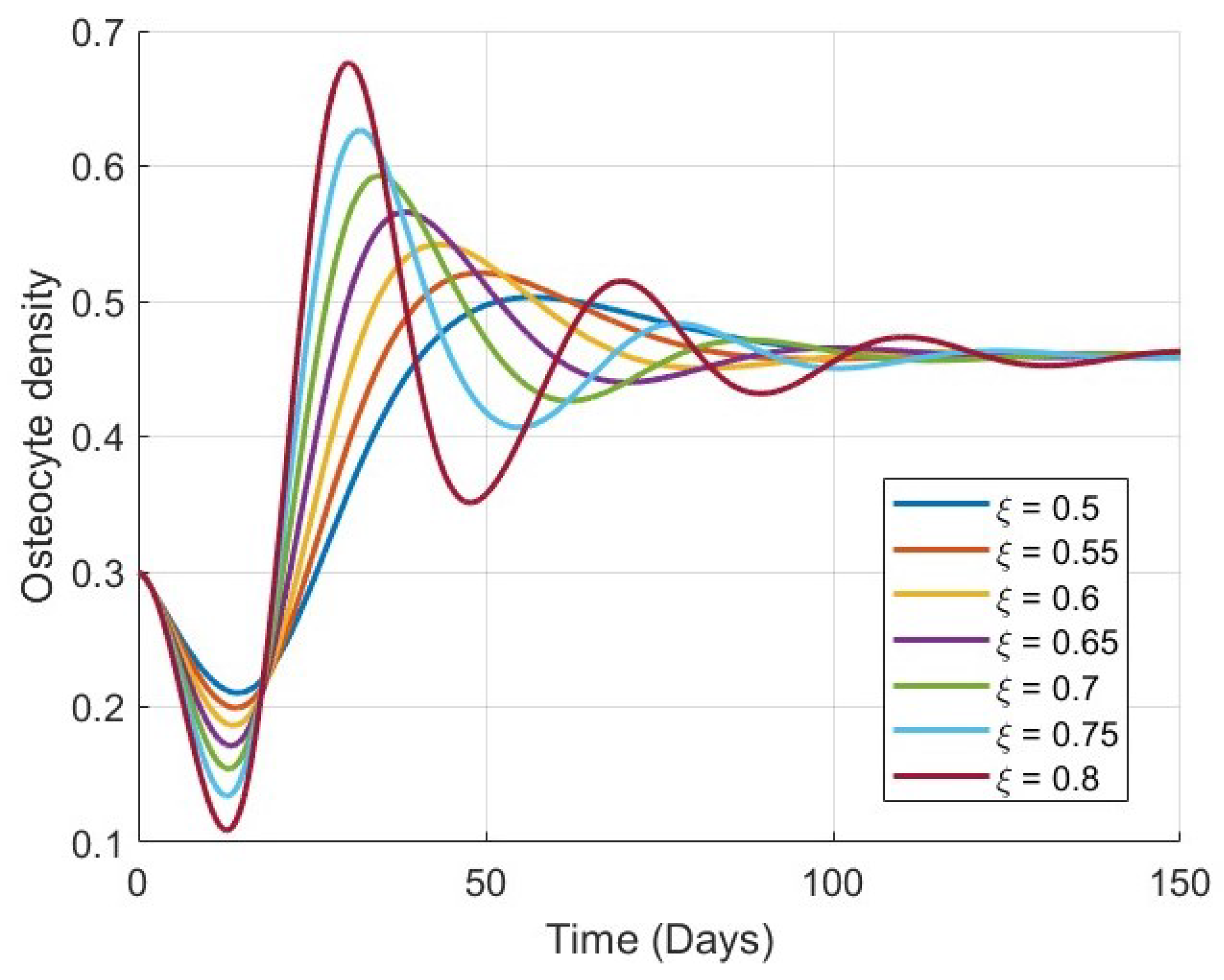
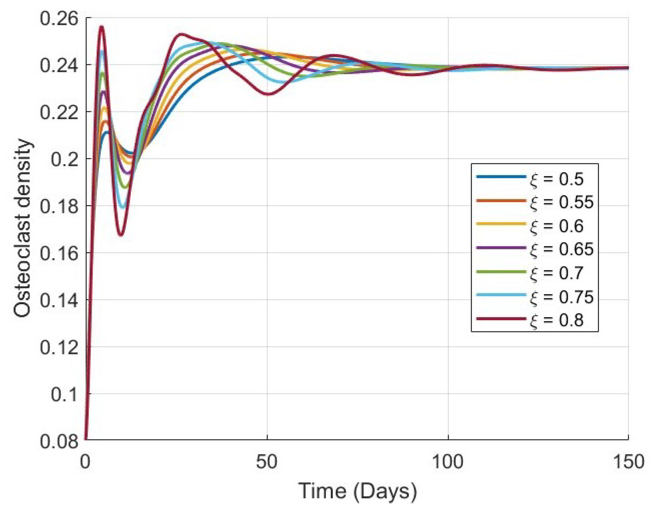
The numerical solutions of the ABC-fractional-order model (3) are presented for a range of fractional orders $\xi =0.5,0.55,0.6,0.65,0.7,0.75,0.8$. Figure 1, Figure 2, Figure 3 and Figure 4 show the time evolution of the key biological variables: osteocyte density $Y\left(t\right)$, osteoblast density $Z\left(t\right)$, osteoclast density $W\left(t\right)$, and bone mass density $\rho \left(t\right)$, respectively. For all considered values of $\xi$, the trajectories of each variable exhibit monotonic or smooth convergence toward the corresponding steady-state values at the equilibrium point $E^{*}=(Y^{*},Z^{*},W^{*},{\rho }^{*})$. This convergence supports the theoretical analysis of global stability and confirms that the model is capable of describing stable long-term bone remodeling behavior.

As $\xi$ increases, the rate at which each variable approaches its equilibrium decreases. This behavior reflects the memory effect inherent in fractional-order systems: lower values of $\xi$ correspond to weaker memory, allowing the system to respond and stabilize more rapidly, while higher $\xi$ values result in stronger memory and delayed convergence. This trend is consistently observed in all four plots, particularly in Figure 4, where the evolution of bone mass density $\rho \left(t\right)$ becomes noticeably slower as $\xi$ increases.

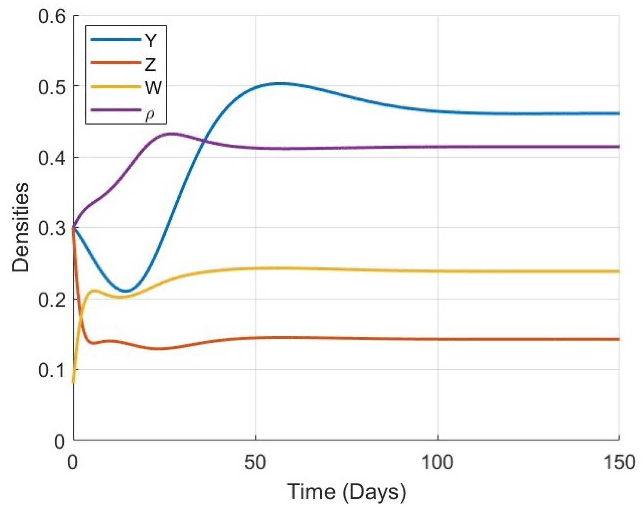
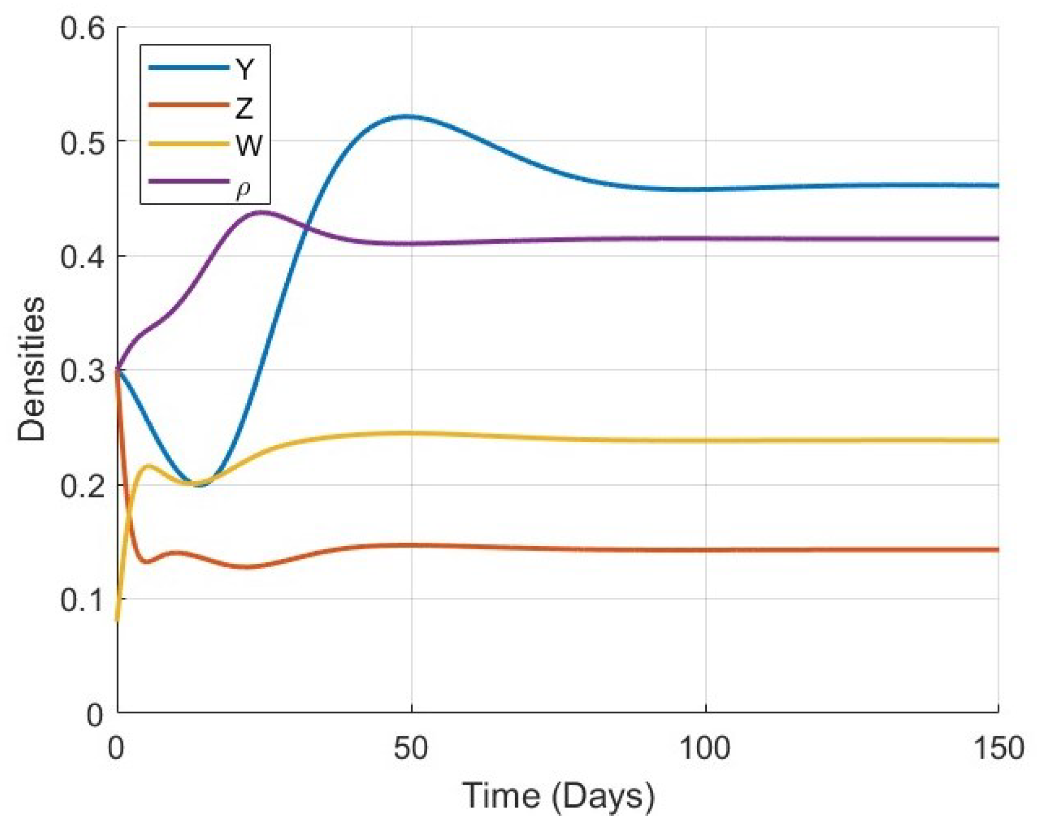
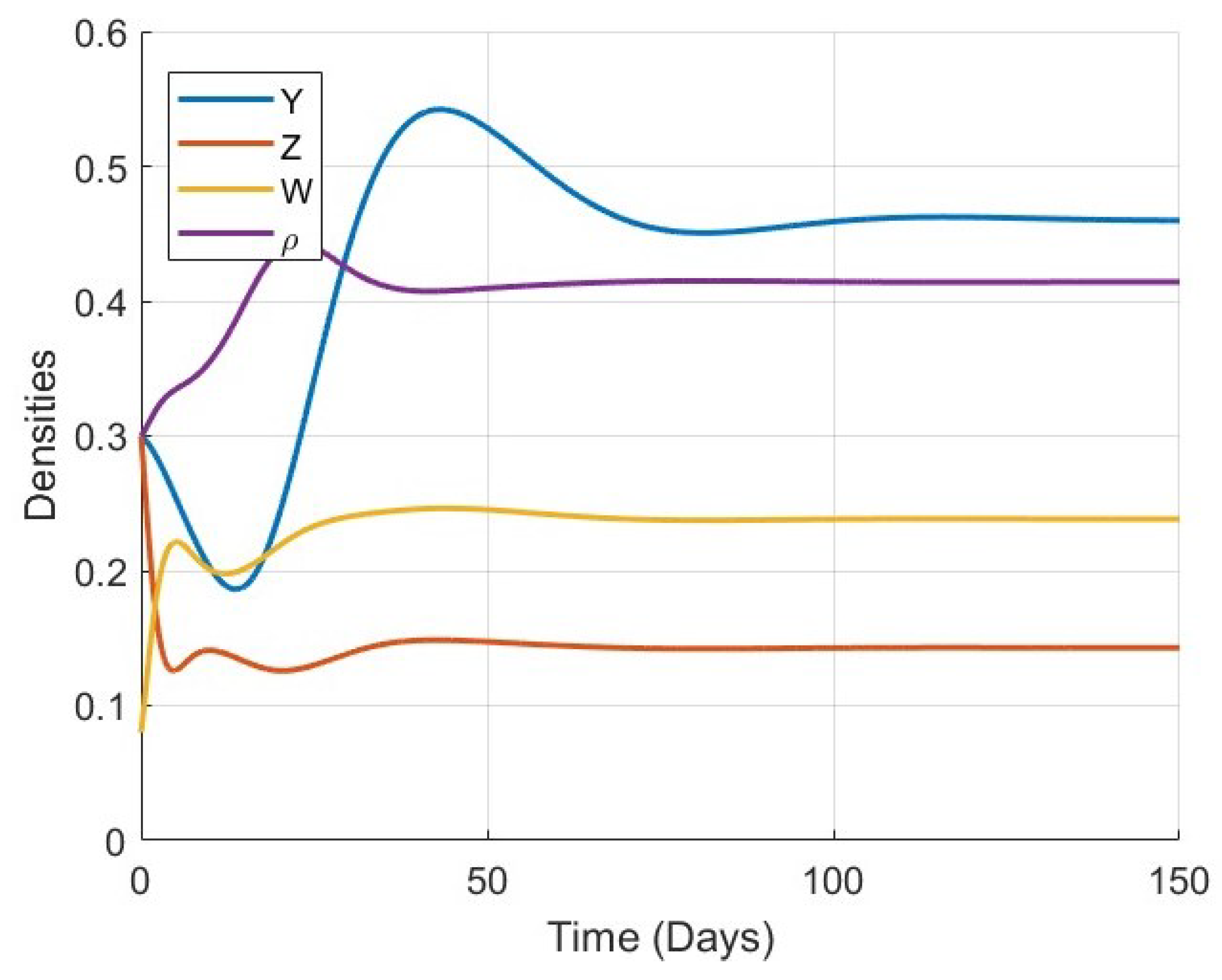
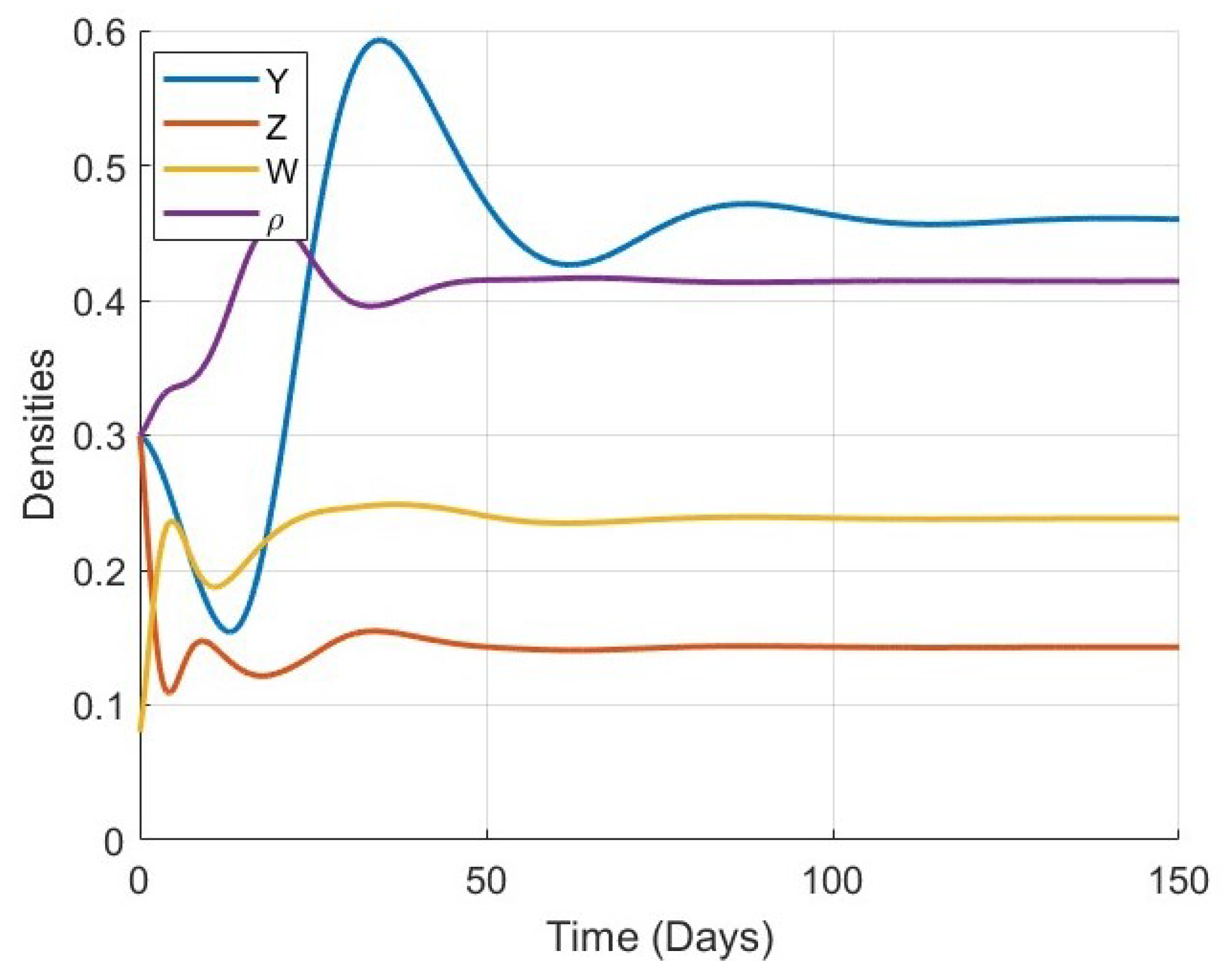
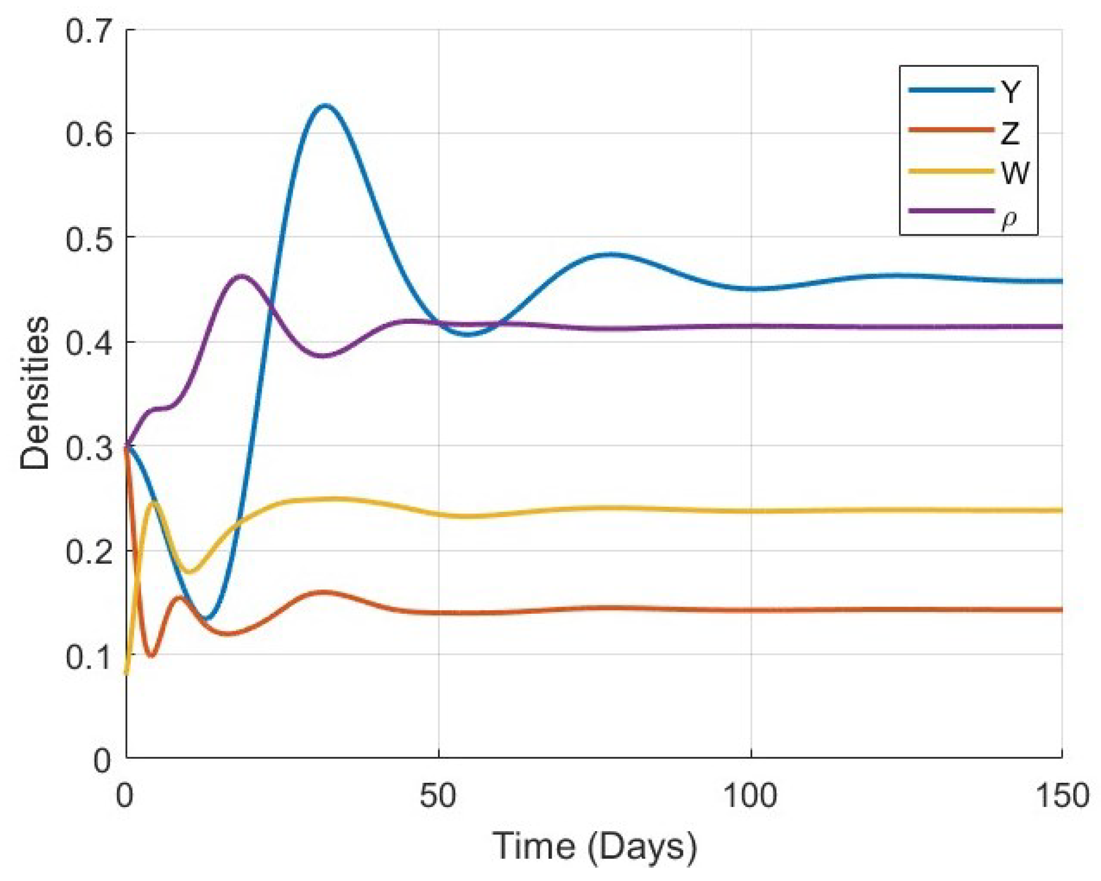
Figure 5, Figure 6, Figure 7, Figure 8, Figure 9, Figure 10 and Figure 11 provide a more detailed view of the system’s behavior for each specific value of $\xi$. Each figure displays the time series of all four variables ($Y\left(t\right),Z\left(t\right),W\left(t\right),\rho \left(t\right)$) in a single plot. These figures illustrate the full trajectory of the bone remodeling process and show that despite the variations in fractional order, the qualitative behavior of the system remains consistent. The populations of osteoblasts, osteoclasts, and osteocytes, as well as the bone mass density, all evolve smoothly and tend toward equilibrium without oscillations or divergence.

These numerical results highlight the significant role of the fractional-order parameter in regulating the speed of convergence and the temporal response of the system. The inclusion of the Atangana–Baleanu–Caputo fractional derivative allows the model to capture the memory-driven characteristics of biological tissue response, offering a more flexible and realistic tool for simulating bone remodeling over time. Overall, the simulations not only validate the analytical results but also demonstrate the practical capability of the model to represent complex biological dynamics under varying memory effects.

6. Conclusions

In this study, we developed a novel mathematical framework for bone remodeling using the Atangana–Baleanu–Caputo (ABC) fractional derivative to incorporate memory effects inherent in biological processes. Our model comprehensively captures the complex interactions among osteoblasts, osteoclasts, osteocytes, and bone mass density through porosity-dependent nonlinear terms that reflect the physiological reality of bone tissue dynamics. We established precise mathematical foundations by proving the positivity, existence, and uniqueness of solutions within biologically feasible domains. The identification of equilibrium points and their global stability analysis using carefully constructed Lyapunov functions demonstrated that the system converges to steady states regardless of initial conditions, ensuring biological consistency and predictive reliability. Numerical simulations across various fractional-order parameter values validated our analytical results and revealed how memory effects influence convergence rates and system dynamics. The fractional-order approach proved superior to classical integer-order models by providing more realistic representations of bone remodeling processes. The memory kernel inherent in the ABC derivative captures the hereditary nature of cellular responses, where current bone formation and resorption rates depend on historical cellular activities. This enhanced modeling capability offers significant improvements in accuracy and biological relevance compared to traditional ordinary differential equation models. Our findings demonstrate that fractional-order modeling constitutes a powerful tool for biomedical applications, particularly in understanding complex physiological processes characterized by memory effects and long-range dependencies. However, the model’s limitations include the use of fixed parameter values that may not account for substantial inter-individual variability in bone metabolism, and the exclusion of critical factors such as hormonal regulation, mechanical loading, and spatial heterogeneity that significantly influence bone remodeling dynamics. Despite these constraints, the model’s ability to maintain global stability while incorporating realistic biological constraints makes it suitable for clinical applications and therapeutic intervention studies, offering valuable insights for further studies in biomedical modeling and bone health prediction.

Future research directions should focus to advance fractional-order bone remodeling models. Multi-scale integration could extend the current cellular-level ABC fractional model to incorporate molecular signaling pathways and tissue-level mechanical feedback, creating a comprehensive hierarchical framework that links genetic factors to macroscopic bone properties through memory-dependent dynamics. Spatial heterogeneity modeling using partial fractional differential equations with ABC derivatives could capture site-specific bone remodeling variations between cortical and trabecular regions, accounting for mechanical loading patterns and anatomical differences that influence local cellular activities over time.