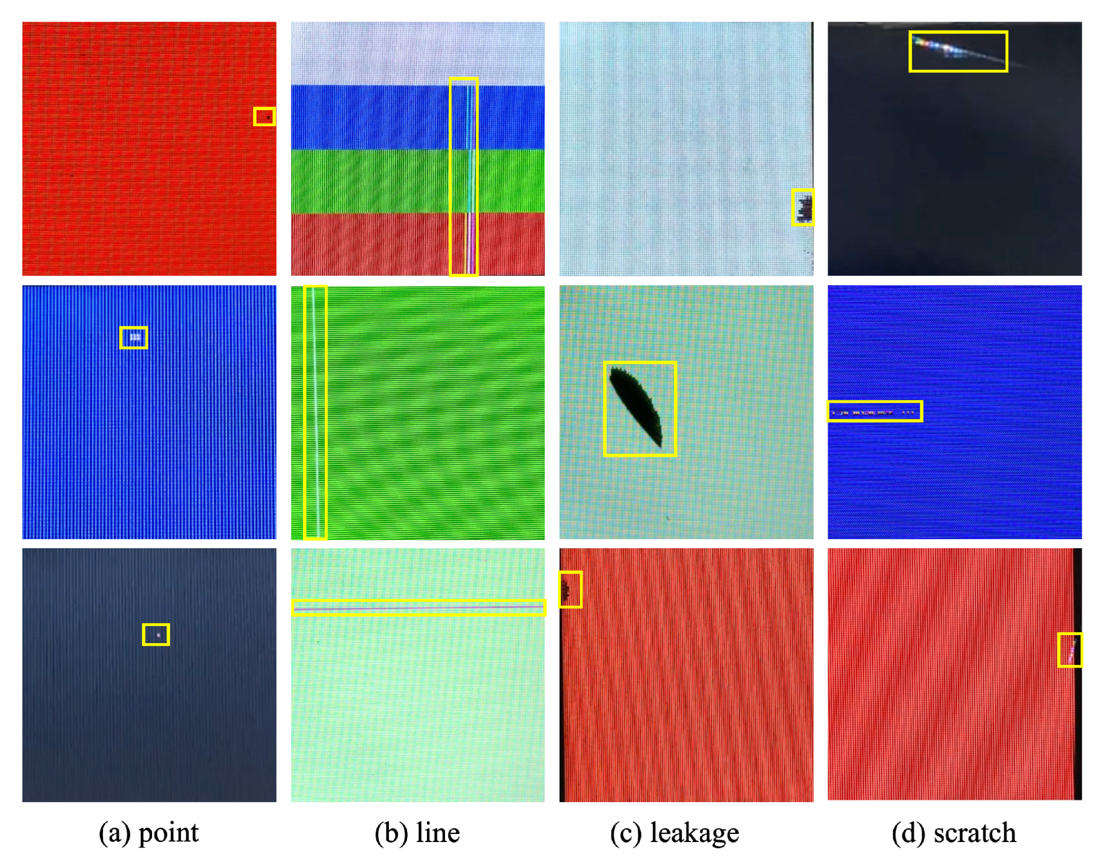
Article

An LCD Defect Image Generation Model Integrating Attention Mechanism and Perceptual Loss

1
School of Electrical and Information Engineering, Wuhan Institute of Technology, Wuhan 430205, China
2
Hubei Key Laboratory of Digital Finance Innovation, Hubei University of Economics, Wuhan 430205, China
3
School of Information Engineering, Hubei University of Economics, Wuhan 430205, China
4
Hubei Internet Finance Information Engineering Technology Research Center, Hubei University of Economics, Wuhan 430205, China
5
Nancheng County Institute of Machine Vision Industry Technology, Fuzhou 344700, China
*
Author to whom correspondence should be addressed.
Current address: School of Electrical and Information Engineering, Wuhan Institute of Technology, No. 206, Guanggu 1st Road, East Lake New Technology Development Zone, Wuhan 430205, China.
These authors contributed equally to this work.
Symmetry 2025, 17(6), 833; https://doi.org/10.3390/sym17060833
Submission received: 22 April 2025 / Revised: 10 May 2025 / Accepted: 14 May 2025 / Published: 27 May 2025
(This article belongs to the Section Engineering and Materials)

Abstract

:
With the rise of smart manufacturing, defect detection in small-size liquid crystal display (LCD) screens has become essential for ensuring product quality. Traditional manual inspection is inefficient and labor-intensive, making it unsuitable for modern automated production. Although machine vision techniques offer improved efficiency, the lack of high-quality defect datasets limits their performance. To overcome this, we propose a symmetry-aware generative framework, the Squeeze-and-Excitation Wasserstein GAN with Gradient Penalty and Visual Geometry Group(VGG)-based perceptual loss (SWG-VGG), for realistic defect image synthesis.By leveraging the symmetry of feature channels through attention mechanisms and perceptual consistency, the model generates high-fidelity defect images that align with real-world structural patterns. Evaluation using the You Only Look Once version 8(YOLOv8) detection model shows that the synthetic dataset improves mAP@0.5 to 0.976—an increase of 10.5% over real-data-only training. Further assessment using Peak Signal-to-Noise Ratio (PSNR), Structural Similarity Index Measure (SSIM), Root Mean Square Error (RMSE), and Content Similarity (CS) confirms the visual and structural quality of the generated images.This symmetry-guided method provides an effective solution for defect data augmentation and aligns closely with Symmetry’s emphasis on structured pattern generation in intelligent vision systems.

1. Introduction

With the increasing integration of intelligent technologies, small-sized liquid crystal displays (LCDs) have become critical interactive interfaces. This trend is driving a surge in demand for such displays. However, manufacturing defects such as point defects, line defects, liquid leakage, and scratches are inevitable (Figure 1).Currently, defect inspection primarily relies on manual quality control. This process is labor-intensive, time-consuming, and inadequate for the real-time detection requirements of intelligent production lines. As a result, it has become a bottleneck in production capacity.
The advancement of machine vision has facilitated the development of intelligent defect detection methods [1,2,3], including You Only Look Once(YOLO) [4] and Faster Region-based Convolutional Neural Network(Faster R-CNN) [5]. However, the effectiveness of these methods heavily depends on the availability of high-quality and well-balanced datasets [6,7]. Figure 2 illustrates the data distribution from an LCD screen production factory. It reveals that point defects and scratches are common, whereas line defects and liquid leakage are rare, leading to a highly imbalanced dataset.Studies have shown that data augmentation can significantly enhance defect detection performance, especially in imbalanced datasets [8,9,10]. Traditional techniques such as geometric transformations and brightness adjustments can increase data volume. However, they struggle to improve sample diversity.In contrast, intelligent data generation methods offer promising solutions. These include Generative Adversarial Networks (GANs) [11], Variational Autoencoders (VAEs) [12], and Denoising Diffusion Probabilistic Models (DDPMs) [13]. Among them, GANs have become a mainstream approach due to their efficiency and ability to generate diverse samples [14,15,16]. However, applying GANs directly to LCD defect generation presents several challenges. The scarcity of real defect samples leads to unstable training. In addition, complex defect details are difficult to synthesize accurately, and conventional architectures often fail to capture deep hierarchical features effectively.
To address these issues, researchers have proposed several GAN-based improvements. Conditional GANs (CGANs) [17] use label information to guide image generation. Deep Convolutional Generative Adversarial Network(DCGAN) [18] enhance feature extraction through convolutional designs. Wasserstein Generative Adversarial Network [19] optimize the loss function, and Wasserstein Generative Adversarial Network with Gradient Penalty(WGAN-GP) [20] introduces gradient penalty to stabilize training.Despite these advancements, WGAN-GP still struggles to generate complex defects such as liquid leakage.Recently, attention mechanisms have shown remarkable potential in improving image generation quality. The Squeeze-and-Excitation (SE) module [21], for example, adaptively adjusts channel weights to emphasize important regions. Inspired by this, we integrate the SE module into the WGAN-GP generator. This enables the model to focus more effectively on defect regions and improves the fidelity of the generated images.
Furthermore, traditional pixel-wise loss functions often fail to capture high-level semantic information. This shortcoming can result in perceptual distortions in generated images. Perceptual loss [22] addresses this issue by using features extracted from a pre-trained network. Therefore, we construct a perceptual loss function based on Visual Geometry Group(VGG)-19 to enhance the structural realism of generated defect images.
In summary, a novel defect image generation model, Squeeze-and-Excitation Wasserstein GAN with Gradient Penalty and VGG-based perceptual loss (SWG-VGG), is proposed based on WGAN-GP. The main contributions of this work are as follows:
  • The SE attention mechanism is integrated into the generator to enhance the model’s ability to focus on key defect regions.
  • A perceptual loss based on VGG-19 is introduced to improve the structural realism and perceptual quality of generated images.
  • A defect dataset of small-sized LCD modules is constructed, providing data support for model training and evaluation.

2. Related Theoretical Basis

2.1. Generative Adversarial Networks

Generative Adversarial Networks (GANs) were proposed by Ian Goodfellow et al. [11] in 2014. The core idea of GANs is to train a generator and a discriminator in an adversarial manner, enabling the generator to produce increasingly realistic data. The basic structure of GANs is illustrated in Figure 3.
A GAN consists of a generator and a discriminator. The generator receives a random noise vector sampled from a Gaussian or uniform distribution and maps it to the target data space using transposed convolution operations, aiming to generate realistic synthetic data that can deceive the discriminator. The discriminator, a binary classification network, employs a convolutional neural network (CNN) to extract features from the input data and outputs a probability value via fully connected layers to determine whether the input is real or generated.
The training of GANs follows a minimax game, where the generator attempts to minimize the discriminator’s ability to distinguish real from generated data, while the discriminator aims to maximize its classification accuracy. The objective function is defined as follows:
min G max D V ( D , G ) = E x p data ( x ) [ log D ( x ) ] + E z p z ( z ) [ log ( 1 D ( G ( z ) ) ) ]
where D ( x ) denotes the discriminator’s output for real data x, D ( G ( z ) ) is the output for generated data G ( z ) , p data represents the real data distribution, and p z denotes the distribution of input noise. During training, the generator and discriminator are alternately optimized until a Nash equilibrium is reached, making it difficult to distinguish generated samples from real ones.

2.2. Channel Attention Mechanism

The channel attention mechanism is a type of attention strategy in deep learning designed to assign adaptive weights to different feature channels, thereby allowing the network to focus on the most informative channels for a given task. In convolutional neural networks (CNNs), feature maps are composed of multiple channels, each potentially representing specific types of features such as edges or textures. However, not all channels contribute equally to the task at hand. Channel attention aims to enhance relevant features and suppress less useful ones through a learned weighting process.
Typically, the mechanism involves three main stages: feature aggregation, weight generation, and channel reweighting. First, global average pooling is applied to compress the spatial information of each channel into a single descriptor, capturing global contextual information. Then, a lightweight transformation—often involving a sigmoid activation function—is used to generate attention weights for each channel. Finally, these weights are applied to the original feature maps to modulate the response of each channel accordingly. This mechanism improves the network’s ability to highlight task-relevant features and has been widely adopted in tasks such as image classification and object detection.

2.3. Perceived Loss

Perceptual loss is a high-level semantic loss function commonly used in image generation and image-to-image translation tasks. Unlike traditional pixel-wise losses, such as mean squared error, perceptual loss emphasizes the visual and semantic similarity between generated and target images. It has been widely employed in applications such as style transfer, super-resolution, and image denoising, where maintaining structural and perceptual fidelity is crucial.
This loss is computed by passing both the generated and reference images through a pretrained convolutional neural network (e.g., VGG) and comparing their high-level feature representations at specific layers. Content loss is defined as the discrepancy between the feature representations of the two images, ensuring that the generated image retains the structural layout and semantic information of the target. In contrast, style loss measures the differences in feature correlations—typically captured by Gram matrices—thereby ensuring consistency in texture, color, and overall style.
The final perceptual loss is often formulated as a weighted combination of content and style losses, enabling the model to generate visually plausible images that are both semantically meaningful and stylistically coherent.

3. Methods

3.1. Structural Overview

The proposed SWG-VGG model is based on WGAN-GP, designed to address complex defect morphology and image distortion in small-size display screens. The overall framework is shown in Figure 4, consisting of a generator, a discriminator, and VGG-19.
During training, the generator receives a 100-dimensional noise vector sampled from a standard normal distribution and maps it through deconvolution layers to generate 256 × 256 defect images. The discriminator differentiates real from generated images and computes the WGAN-GP loss to improve the generator. VGG-19 extracts high-level features from both real and generated images, computing the perceptual loss, ensuring generated images maintain realistic textures and structures.

3.2. Generator and Discriminator Design

The traditional WGAN architecture usually suffers from low image quality and missing details when generating high-resolution images. In order to solve these problems, improve the quality of generated images, and enhance the ability to capture key features, this paper redesigns the generator structure, as shown in Figure 5.
The generator structure mainly consists of five parts:
  • The input layer, namely, the noise mapping layer, is responsible for accepting the 100-dimensional random noise vector Z and mapping it to a high-dimensional feature space to provide initial features for generating images.
  • The upsampling part, including multiple transposed convolution layers and nonlinear activation layers, gradually expands the resolution of the feature map to the target size.
  • The channel attention layer is responsible for adjusting the channel weights of generated feature maps so that the model can more accurately capture the key features of the image.
  • The high-resolution feature reconstruction part: The feature maps are further upsampled, and the number of channels is gradually reduced so that the high-resolution features match the target output size.
  • The output layer: A transposed convolution layer is used to convert the feature map into the target image channel number of RGB three channels, and the pixel value is restricted to the range of [−1, 1] through the Tanh activation function.
The generator structure is composed of several 4 × 4 deconvolution layers and SELayer. This paper embeds SELayer into the generator and expands the structure of the generator, increasing the resolution of the output image from 64 × 64 to 256 × 256, greatly enhancing the detail expression ability of the defect image. Each block contains a deconvolution layer, a batch normalization layer, a ReLU(rectified linear unit) activation function layer, and a SELayer. The role of these layers is to gradually amplify the low-resolution features and use the attention mechanism to optimize the feature expression of the channel. The workflow of the generator is to first use the deconvolution operation to upsample the input feature map and extract important features. The calculation process can be expressed as:
H out = ( H in 1 ) s 2 p + k ,
where H out and H in are the heights of the output and input feature maps, respectively, s is the stride, p is the padding size, and k is the convolution kernel size. Then the output feature map is batch normalized to standardize the feature maps of each batch, reduce the internal covariance shift during training, and thus accelerate convergence and stabilize training. For each feature channel, the batch normalization operation can be expressed as:
x ^ = x μ σ 2 + ϵ ,
y = γ x ^ + β ,
where x is the output feature map, ϵ is a small constant to prevent division by zero, γ and β is a learnable parameter for translation and scaling. Then, nonlinearity is introduced through the ReLU activation function to enhance the feature expression capability. Finally, a SELayer is used to enhance the expression capability of channel features.
The SE module is a channel attention module used to improve the performance of convolutional neural networks. In the display defect image generation task, the SE module can weight the importance of each channel, thereby enhancing the generator’s attention to the defect morphology to improve the clarity of the generated defect image. The structure of the SE module is shown in Figure 6.
First, the input feature map X is transformed into a feature map U through a standard convolution operator Ftr, that is, each layer of the input feature map X is convolved with a 2D spatial kernel to finally obtain C output feature maps to form the feature map U. Then the compression operation is performed, that is, the global spatial information is compressed into a channel descriptor, and the feature map U containing the global information is compressed into a 1 × 1 × C feature vector using the global average pooling of the channel. The specific operation is defined as:
F sq ( u c ) = 1 H × W i = 1 H j = 1 W u c ( i , j ) ,
where u c ( i , j ) represents ( i , j ) the value of channel c at the spatial position, and indicates the use of global average pooling of the channel. After feature compression, the obtained channel descriptor is input into the weight generation network for weight generation to learn the weight of each channel. Weight generation is divided into two steps. First, the channel descriptor passes through the first fully connected layer and uses the ReLU activation function to reduce the feature dimension to the original C / r , where r is the scaling factor. Then the dimension is restored to C through the second fully connected layer, and the Sigmoid activation function is used to limit the weight to the range of [0, 1]. Each channel will get a corresponding weight to indicate its importance in the current task. The weight generation process can be expressed as:
F ex ( z , W ) = σ ( W 2 δ ( W 1 z ) ) ,
where z is the channel descriptor vector, W 1 and W 2 are the weight matrices of the two fully connected layers, δ and σ represent the ReLU and Sigmoid activation functions respectively, and s is the channel weight vector. Finally, the generated channel weight s is multiplied by the original feature map channel by channel to achieve the final feature weighted output. The feature weighting can be expressed as:
F scale ( u c , s c ) = s c u c ,
where s c is the weight of the c th channel, is the value of the original feature map in channel c, and finally outputs the weighted feature map.
In WGAN-GP, the discriminator’s goal is different from that of traditional GAN. The discriminator of WGAN-GP uses Wasserstein distance instead of cross entropy loss. WGAN-GP optimizes the adversarial relationship between the generator and the discriminator by minimizing the Wasserstein distance. In order to ensure the Lipschitz continuity of the discriminator, WGAN-GP also introduces gradient penalty.
The WGAN-GP discriminator replaces cross-entropy loss with Wasserstein distance and includes a gradient penalty term to enforce Lipschitz continuity. Its structure, shown in Figure 7, processes 3 × 256 × 256 images through five convolution blocks, each containing a convolution layer, batch normalization, and LeakyReLU activation, followed by a final 4 × 4 convolution layer outputting a real/fake score. The Wasserstein loss and gradient penalty are computed as:
L D = E x r P data [ D ( x r ) ] E x g P g [ D ( x g ) ] ,
L GP = λ E x ^ P x ^ [ ( x ^ D ( x ^ ) 2 1 ) 2 ] ,
where x ^ is an interpolated sample between real and generated images.

3.3. Loss Function Improvement

The loss function of the original WGAN-GP model cannot fully capture the high-level semantic information of the image. Therefore, this model introduces perceptual loss to improve the problem of image distortion generated by the generator. Perceptual loss uses VGG-19 to extract high-level features of the generated image and the real image to calculate the difference between these features, and finally weighted sums the feature differences of different layers to obtain the final perceptual loss. The calculation flow chart of perceptual loss is shown in Figure 8.
First, the input image X is passed through a generative network to output a picture. The VGG network extracts the feature map of the input image, and then calculates the mean square error between the style image and the content image and the generated image to obtain the loss function L style , L feat . Finally, the weight of the conversion network is adjusted according to the loss value to output the image y h . This model uses the middle five convolutional layers of VGG-19 to extract image features, and uses Conv1_1, Conv2_1, Conv3_1, Conv4_1, and Conv5_1 to calculate style losses at different levels L style , and uses Conv3_1 to calculate content losses, L feat which are combined into perceptual losses L p . The calculation process can be expressed as:
L style = l 1 C l 2 H l 2 W l 2 i = 1 C l j = 1 C l ( G l ( y h ) ) i j ( G l ( y s ) ) i j 2 ,
L feat = 1 C 3 H 3 W 3 i = 1 C 3 j = 1 H 3 k = 1 W 3 φ 3 ( y h ) i j k φ 3 ( y c ) i j k 2 ,
L p = L style + L feat ,
where l is the set of feature layers, C l , H l , W l are the number of channels, height and width of the feature map, respectively, y h is the generated image, y s is the style image, G j is the Gram matrix calculated for the target image, φ 3 represents the feature map of the image at layer 3. The total loss function of this paper combines the WGAN-GP loss with the perceptual loss and is defined as follows:
L total = L WGAN - GP + α ( t ) L p ,
where α ( t ) is the weight coefficient of perceptual loss, which is used to adjust the weight of perceptual loss in the overall loss. Through experimental analysis, the model loss convergence process is best when this value is set to 0.001.

4. Experiments

4.1. Experimental Environment and Dataset

To validate the effectiveness of the proposed method, three sets of experiments were conducted.All experiments were implemented using the PyTorch (version 1.13.1) framework. The hardware device was a 12th Generation Intel Core i5-12400F CPU (Intel Corporation, Santa Clara, CA, USA), an NVIDIA GeForce RTX 3080 Ti GPU (NVIDIA Corporation, Santa Clara, CA, USA), and a Windows 11 system with 12 GB RAM.
The dataset used in this study consists of defect images of LCD screens, collected on-site in a factory setting. To ensure data authenticity and diversity, images were captured from different production batches under real manufacturing conditions. The defect inspection process requires the display to be fully illuminated, as defect visibility varies across different background colors. Therefore, each defect was captured under five background conditions: white, blue, green, red, and colorful, ensuring no defects appeared in these backgrounds. For line defects, black refers to cases where the screen fails to illuminate properly and bright lines appear. Since leakage defects are inherently black, they are not visible against black backgrounds, and thus, no leakage defect samples were collected under such conditions.
For each defect, 30 different images were collected under each background color, and finally a multi-background and multi-view defect image dataset was constructed as shown in Table 1. A high-resolution industrial camera was used for data acquisition. The dataset includes defect images from multiple production lines and varying process conditions, ensuring its representativeness.

4.2. Evaluation Metrics

In this study, to comprehensively evaluate the quality of generated images, several commonly used image quality metrics were selected, including Peak Signal-to-Noise Ratio (PSNR) [23], Structural Similarity Index Measure (SSIM) [24], Root Mean Square Error (RMSE), and Content Similarity (CS). PSNR is mainly used to measure the pixel-level difference between the generated image and the real image. A higher PSNR value indicates a lower degree of distortion; SSIM evaluates the structural similarity of the image by comparing the brightness, contrast and structural information of the image. The closer the SSIM value is to 1, the more similar the images are; RMSE is used to measure the pixel-level difference between the generated image and the real image. The smaller the RMSE, the smaller the difference between the generated image and the real image, and the higher the image quality; finally, CS is used to measure the similarity between the generated image and the real image. A higher CS value indicates that the overall quality of the generated image is closer to the real image. These indicators are defined as:
PSNR = 10 · log 10 ( MAX 2 MSE ) ,
SSIM = ( 2 μ x μ y + c 1 ) ( 2 σ x y + c 2 ) ( μ x 2 + μ y 2 + c 1 ) ( σ x 2 + σ y 2 + c 2 ) ,
RMSE = 1 n i = 1 n ( x i y i ) 2 ,
CS = x · y x y ,
where x and y represent the generated image and the original image respectively, x i and y i are the pixel values of the generated image and the original image at position i, MAX is the maximum pixel value of the image, which is usually 255 for 8-bit images, and MSE is the mean square error. μ and σ 2 represent the mean and variance of the image respectively, c 1 and c 2 are constants. x and y are the norms of x and y.

4.3. Experimental Results and Analysis

4.3.1. Ablation Analysis

To validate the effectiveness of the proposed model, several ablation experiments were conducted by progressively adding the SE module and perceptual loss to assess their contributions to image quality. The experiments were based on a small-sized LCD screen defect image dataset with a resolution of 256 × 256, using PSNR, SSIM, MI, and CS as evaluation metrics. Four models were compared: Model 1 is the traditional WGAN-GP (baseline model); Model 2 adds the SE module to the baseline model; Model 3 introduces perceptual loss; Model 4 incorporates both the SE module and perceptual loss. The experiments were conducted in the same environment using the same dataset to generate defect images, with the average metrics of leakage and line defect images shown in Table 2 and the generator loss curves depicted in Figure 9. In order to better demonstrate the impact of each module on the model, this paper statistically compares the scores of each indicator of each model at different training stages. Table 3 is the score comparison of leakage defects at different training stages, and Table 4 is the score comparison of line defects at different training stages; Figure 10 and Figure 11 are the comparisons of leakage defect and line defect images generated when the model is trained to different stages.
The results show that:Compared to Model 1, Model 2 outperforms in all metrics, with PSNR, SSIM, and CS improving by 0.57, 0.0104, and 0.014, respectively, and RMSE decreasing by 1.1001. Table 3 and Table 4 show that after 1900 epochs, Model 2 generates higher-quality defect images. The SE module enhances image details in terms of brightness, contrast, and structural features, and the loss curve converges faster. Model 3, compared to Model 1, improves PSNR, SSIM, and CS by 0.39, 0.0212, and 0.0097, respectively, with RMSE reduced by 0.7345. The perceptual loss enhances image quality, and the loss value is lower than that of Models 1 and 2.Compared to Model 1, Model 4 improves PSNR, SSIM, and CS by 1.6, 0.0417, and 0.0442, respectively, and reduces RMSE by 1.7238. In most training stages, Model 4 outperforms the other models across all four metrics, with faster convergence of the generator loss, and the loss value is the same as Model 3. Figure 10 and Figure 11 show that Model 4 generates higher-quality and more detailed leakage and line defect images than the other models.
In conclusion, both the SE module and perceptual loss individually improve image quality, while their combination significantly enhances the model’s performance. This confirms that the integration of the SWG-VGG architecture with perceptual loss substantially improves the quality of defect image generation for small-sized LCD screens.

4.3.2. Comparative Analysis

To comprehensively evaluate the performance of the proposed SWG-VGG model, comparative experiments were conducted with the classic WGAN-GP and DCGAN models. Using the dataset shown in Table 1, the performance of the three models in generating line and leakage defect images was tested. The experiments were carried out in the same environment with the same computer and dataset, using these three generative models for defect image generation. The results, including PSNR, SSIM, RMSE, and CS metrics, are shown in Table 5, and the average scores of generated images are provided in Table 6. The scores of randomly generated 200 line and leakage defect images, as well as their comparison across different backgrounds, are shown in Figure 12 and Figure 13, with image comparisons in Figure 14.
The results indicate that the SWG-VGG model outperforms the other two models in PSNR, SSIM, RMSE, and CS scores for both line and leakage defect images. The leakage defect images scored 23.7, 0.83, 19.13, and 0.84, while the line defect images scored 23.41, 0.78, 22.92, and 0.81, with average scores of 23.56, 0.80, 21.02, and 0.83. Compared to the WGAN-GP model, the PSNR, SSIM, and CS values improved by 1.6, 0.04, and 0.05, respectively, while RMSE decreased by 1.73. Table 5 shows that the SWG-VGG model scores significantly better than WGAN-GP. Compared to the DCGAN model, SWG-VGG improved PSNR, SSIM, and CS by 1.13, 0.03, and 0.04, respectively, with RMSE decreased by 0.81. The scatter plots in Figure 12 show that SWG-VGG outperforms DCGAN, especially in terms of RMSE, while other metrics are slightly better than those of DCGAN.
Figure 13 show that for leakage defects, SWG-VGG achieves the highest PSNR across all backgrounds. WGAN-GP and DCGAN have lower PSNR, particularly on white and red backgrounds, where WGAN-GP performs the worst. SSIM follows a similar trend among the three models, with SWG-VGG achieving the best structural similarity, always higher than the other two models. DCGAN performs better than WGAN-GP, especially on colorful and white backgrounds. SWG-VGG also has the lowest RMSE, indicating minimal error in image generation. WGAN-GP consistently has the highest RMSE, indicating the greatest error in generated images. The CS value is highest for SWG-VGG, confirming the highest correlation between the generated images and reference images. For line defects, SWG-VGG performs best in PSNR, but background color has a significant impact, particularly with slight performance drops on white and red backgrounds. SSIM and CS are also higher in SWG-VGG, especially on black and blue backgrounds, demonstrating its stability. WGAN-GP performs the worst, particularly in RMSE and CS, highlighting its deficiencies in generating line defect images. Figure 14 and Figure 15 shows that SWG-VGG generates defect images with high fidelity in terms of color, texture, and structure, accurately capturing defect targets. WGAN-GP-generated line defect images on colorful and white backgrounds show distortion, while DCGAN-generated images exhibit less distortion but with poorer overall quality.Other line defects and leakage defect images generated by the model proposed in this study are shown in Figure 16.

4.3.3. Application Analysis

To verify the effectiveness of the SWG-VGG model’s generated LCD defect images in practical applications, this study employed the high-performance object detection model YOLOv8 for testing and analysis. YOLOv8 is a single-stage object detection algorithm that strikes a good balance between detection speed and accuracy and is widely used in defect detection. In the experiment, the training set used defect images generated by the SWG-VGG model, while the validation set used original defect images, with input image sizes uniformly set to 416 × 416. During training, the hyperparameters were set as follows: 50 epochs, batch size of 16, and the Adam optimizer. Model performance on the validation set was evaluated using precision, recall, and mean average precision (mAP@50), with training results shown in Figure 17 and Table 7.
As shown in Figure 17,the YOLOv8 model trained with generated data achieved precision, recall, and mAP@50 values of 94.6%, 93.8%, and 97.6%, respectively. In comparison, the model trained with original images performed significantly worse on the same test set, with precision, recall, and mAP@50 values of 89.9%, 74.5%, and 87.1%. The YOLOv8 model trained with generated data showed improvements of 4.7%, 19.3%, and 10.5%, respectively. This discrepancy indicates that the inclusion of the generated dataset, especially with regard to defect sample diversity and quantity, greatly enhanced YOLOv8’s performance. The detection accuracy mAP@50 values in Table 7 show that the average mAP@50 across all defect types in the original dataset was only 0.871, with leakage defects at 0.941, point defects at 0.962, scratches at 0.972, and line defects at 0.609. After incorporating the generated dataset, the model’s overall performance significantly improved, with mAP@50 increasing to 0.976, a 10.5% improvement. The generated data effectively improved the model’s ability to detect weak categories, such as line defects.
In order to further verify the impact of the number of datasets on the stability of the defect detection model, this study designed a series of experiments, using the generated defect image award dataset to be enhanced to 2000, 4000, 6000 and 8000 data for model training and testing. By comparing the performance of the model under different dataset sizes, it aims to explore the specific impact of dataset size on model training effect, accuracy and stability. In the experiment, we mainly focus on the accuracy of the model for four types of defect detection and the stability during training, especially under small dataset conditions, whether the model is prone to overfitting or training instability. Table 8 is a data distribution table in the dataset, and Table 9 is a statistical table of detection accuracy for various types of defects using different datasets.
Table 9 shows that the average accuracy of dataset 2 is 97.8%, which is 0.2% higher than that of dataset 1, and the improvement is small. The line defect accuracy is lower than that of dataset 1, and the point defect accuracy is significantly higher than that of dataset 1, indicating that although the increase in data volume has a small improvement in overall accuracy, it is beneficial to the detection of small-sized defects such as point defects; the average accuracy of dataset 3 is 97.5%, which is roughly the same as dataset 1. The gap in the detection accuracy of various defects has narrowed, and the point defect accuracy is higher than that of dataset 1, indicating that the increase in data volume has increased the stability of the detection model; the average accuracy of dataset 4 reaches the highest, and its point defect accuracy reaches 95.4%, which is significantly higher than the point defect detection accuracy of the first three datasets. The overall improvement is relatively stable, indicating that the increase in the size of the dataset is helpful to improve the detection accuracy of the model, especially when dealing with complex and difficult-to-identify defect types, the expansion of data volume is particularly important.

5. Conclusions

To address the issues of limited defect samples and extreme dataset imbalance for small-sized LCD screens, this study proposes a defect image generation model based on WGAN-GP, named SWG-VGG, which enables accurate generation and detail restoration of line and leakage defects. This model provides an effective and balanced defect sample dataset for intelligent defect detection. Specifically, the model incorporates the Wasserstein distance and gradient penalty mechanism to improve training stability; integrates the SE attention mechanism to enhance the representation of defect areas; expands the generator’s depth and width to better capture fine-grained textures, colors, and shapes; and utilizes VGG-19 to extract deep features and construct perceptual loss, effectively mitigating image distortion during generation.
Ablation studies confirm that each component contributes to improved image quality. The overall model demonstrates significant enhancements across four evaluation metrics (PSNR, SSIM, RMSE, CS), while ensuring stable training and faster convergence. Compared to DCGAN and the standard WGAN-GP, SWG-VGG consistently outperforms in generating high-quality defect images. In application experiments, a defect detection model trained using SWG-VGG-generated samples achieved a substantial accuracy improvement from 87.1% to 97.6%, with especially notable gains in detecting line defects. These results suggest that SWG-VGG has considerable engineering application value in generating realistic defect samples and enhancing intelligent detection systems.
Despite these contributions, the model still faces several limitations. One notable constraint is the fixed or limited placement of defects within generated samples, which may reduce dataset variability and realism. In addition, the current model has not been extensively evaluated on its ability to generalize to unexpected or rare defect types not present in the training data, which could limit its robustness in real-world scenarios with diverse defect patterns.
Future work will focus on addressing these limitations through two main directions. First, we plan to introduce domain adaptation techniques to improve the model’s generalization across different defect domains and enhance its robustness to unseen defect types. Second, we aim to incorporate conditional generation mechanisms or spatial control modules to enable more flexible and controllable placement of defects during generation, thereby increasing the diversity and utility of the generated dataset for downstream detection tasks.

Author Contributions

Conceptualization, S.Z. and Y.Z.; Formal analysis, S.Z., Y.Z. and X.C.; Investigation, S.L.; Methodology, S.Z. and Y.Z.; Project administration, X.C.; Software, S.Z. and Y.Z.; Supervision, S.L.; Validation, S.L.; Visualization, S.Z. and Y.Z.; Writing—original draft, S.Z. and Y.Z.; Writing—review & editing, X.C.; All authors have read and agreed to the published version of the manuscript.

Funding

This research was funded by the Fuzhou Science and Technology Bureau (FZKJ202409ZB04) under the "Jie Bang Gua Shuai" project initiative. The APC was funded by the Fuzhou Science and Technology Bureau.

Data Availability Statement

The data are available on request from the corresponding author. The data are not publicly available due to institutional restrictions.

Conflicts of Interest

The authors declare no conflicts of interest.

References

  1. Li, W.; Zhang, H.; Wang, G.; Xiong, G.; Zhao, M.; Li, G.; Li, R. Deep learning based online metallic surface defect detection method for wire and arc additive manufacturing. Robot. Comput.-Integr. Manuf. 2023, 80, 102470. [Google Scholar] [CrossRef]
  2. Chen, P.; Chen, M.; Wang, S.; Song, Y.; Cui, Y.; Chen, Z.; Zhang, Y.; Chen, S.; Mo, X. Real-time defect detection of TFT-LCD displays using a lightweight network architecture. J. Intell. Manuf. 2024, 35, 1337–1352. [Google Scholar] [CrossRef]
  3. Hu, W.; Xiong, J.; Liang, J.; Xie, Z.; Liu, Z.; Huang, Q.; Yang, Z. A method of citrus epidermis defects detection based on an improved YOLOv5. Biosyst. Eng. 2023, 227, 19–35. [Google Scholar] [CrossRef]
  4. Redmon, J.; Divvala, S.; Girshick, R.; Farhadi, A. You only look once: Unified, real-time object detection. In Proceedings of the IEEE Conference on Computer Vision and Pattern Recognition, Las Vegas, NV, USA, 27–30 June 2016; pp. 779–788. [Google Scholar]
  5. Ren, S.; He, K.; Girshick, R.; Sun, J. Faster r-cnn: Towards real-time object detection with region proposal networks. IEEE Trans. Pattern Anal. Mach. Intell. 2016, 39, 1137–1149. [Google Scholar] [CrossRef] [PubMed]
  6. Lin, S.; Wu, Y. A review of vision-based defect detection methods for LCD/OLED screens. J. Image Graph. 2024, 29, 1321–1345. (In Chinese) [Google Scholar] [CrossRef]
  7. Zhao, L.; Wu, Y. Research progress of surface defect detection methods based on machine vision. Chin. J. Sci. Instrum. 2022, 43, 198–219. [Google Scholar]
  8. Shorten, C.; Khoshgoftaar, T.M. A survey on image data augmentation for deep learning. J. Big Data 2019, 6, 1–48. [Google Scholar] [CrossRef]
  9. Khalifa, N.E.; Loey, M.; Mirjalili, S. A comprehensive survey of recent trends in deep learning for digital images augmentation. Artif. Intell. Rev. 2022, 55, 2351–2377. [Google Scholar] [CrossRef] [PubMed]
  10. Yang, Z.; Sinnott, R.O.; Bailey, J.; Ke, Q. A survey of automated data augmentation algorithms for deep learning-based image classification tasks. Knowl. Inf. Syst. 2023, 65, 2805–2861. [Google Scholar] [CrossRef]
  11. Goodfellow, I.; Pouget-Abadie, J.; Mirza, M.; Xu, B.; Warde-Farley, D.; Ozair, S.; Courville, A.; Bengio, Y. Generative adversarial networks. Commun. ACM 2020, 63, 139–144. [Google Scholar] [CrossRef]
  12. Kingma, D.P.; Welling, M. Auto-encoding variational bayes. arXiv 2013, arXiv:1312.6114v10. [Google Scholar]
  13. Ho, J.; Jain, A.; Abbeel, P. Denoising diffusion probabilistic models. Adv. Neural Inf. Process. Syst. 2020, 33, 6840–6851. [Google Scholar]
  14. Sampath, V.; Maurtua, I.; Aguilar Martin, J.J.; Gutierrez, A. A survey on generative adversarial networks for imbalance problems in computer vision tasks. J. Big Data 2021, 8, 1–59. [Google Scholar] [CrossRef] [PubMed]
  15. Niu, S.; Li, B.; Wang, X.; Lin, H. Defect image sample generation with GAN for improving defect recognition. IEEE Trans. Autom. Sci. Eng. 2020, 17, 1611–1622. [Google Scholar] [CrossRef]
  16. Gao, S.; Dai, Y.; Xu, Y.; Chen, J.; Liu, Y. Generative adversarial network–assisted image classification for imbalanced tire X-ray defect detection. Trans. Inst. Meas. Control 2023, 45, 1492–1504. [Google Scholar] [CrossRef]
  17. Mirza, M.; Osindero, S. Conditional generative adversarial nets. arXiv 2014, arXiv:1411.1784. [Google Scholar]
  18. Radford, A.; Metz, L.; Chintala, S. Unsupervised representation learning with deep convolutional generative adversarial networks. arXiv 2015, arXiv:1511.06434. [Google Scholar]
  19. Arjovsky, M.; Chintala, S.; Bottou, L. Wasserstein generative adversarial networks. In Proceedings of the International Conference on Machine Learning, PMLR, Sydney, Australia, 6–11 August 2017; pp. 214–223. [Google Scholar]
  20. Gulrajani, I.; Ahmed, F.; Arjovsky, M.; Dumoulin, V.; Courville, A.C. Improved training of wasserstein gans. In Proceedings of the 31st International Conference on Neural Information Processing Systems, Long Beach, CA, USA, 4–9 December 2017; Volume 30. [Google Scholar]
  21. Hu, J.; Shen, L.; Sun, G. Squeeze-and-excitation networks. In Proceedings of the IEEE Conference on Computer Vision and Pattern Recognition, Salt Lake City, UT, USA, 18–23 June 2018; pp. 7132–7141. [Google Scholar]
  22. Johnson, J.; Alahi, A.; Li, F.-F. Perceptual losses for real-time style transfer and super-resolution. In Proceedings of the Computer Vision–ECCV 2016: 14th European Conference, Amsterdam, The Netherlands, 11–14 October 2016; Part II 14. Springer: Berlin/Heidelberg, Germany, 2016; pp. 694–711. [Google Scholar]
  23. Wang, Z.; Bovik, A.C.; Sheikh, H.R.; Simoncelli, E.P. Image quality assessment: From error visibility to structural similarity. IEEE Trans. Image Process. 2004, 13, 600–612. [Google Scholar] [CrossRef] [PubMed]
  24. Snell, J.; Ridgeway, K.; Liao, R.; Roads, B.D.; Mozer, M.C.; Zemel, R.S. Learning to generate images with perceptual similarity metrics. In Proceedings of the 2017 IEEE International Conference on Image Processing (ICIP), Beijing, China, 17–20 September 2017; pp. 4277–4281. [Google Scholar]
Figure 1. Examples of typical display defect types and their manifestations. The yellow boxes indicate the defect locations. The images are shown under different background colors to better illustrate defect visibility.
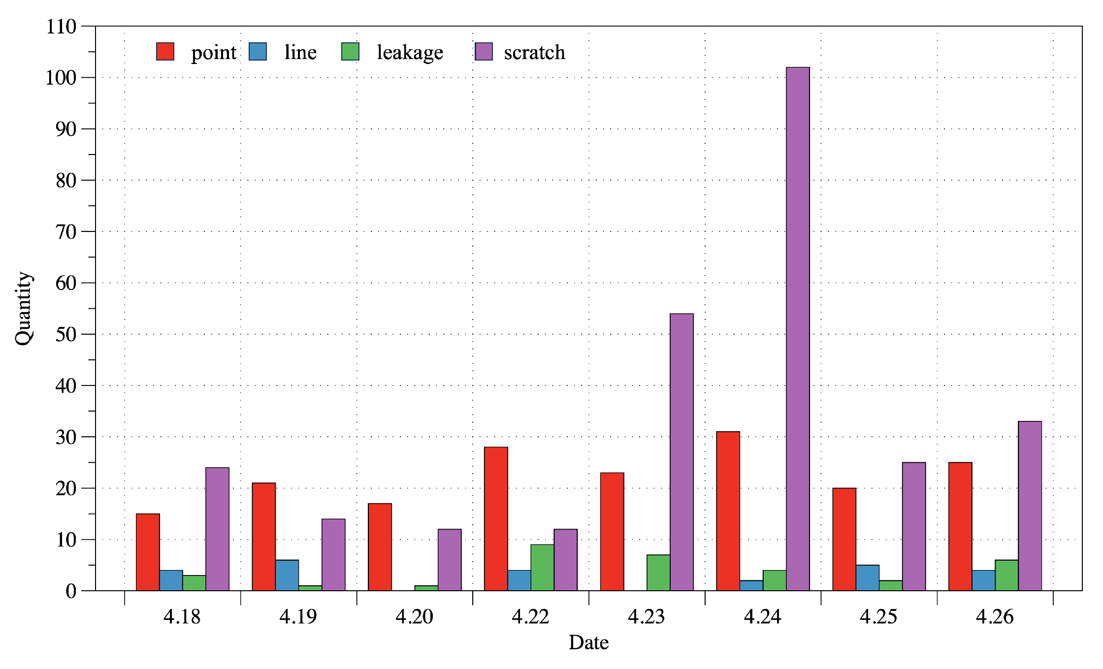
Symmetry 17 00833 g001
Figure 2. Distribution of various defect data generated by a certain LCD display manufacturing plant from 18 April to 26 April 2024.
Symmetry 17 00833 g002
Figure 3. Basic structure of GAN.
Symmetry 17 00833 g003
Figure 4. The framework of the proposed SWG-VGG model. The left side shows the training phase with SE-enhanced generator and VGG-based perceptual loss; the right side shows the image generation phase.
Symmetry 17 00833 g004
Figure 5. SWG-VGG generator structure.The generator consists of five parts, marked as 1–5 in the figure: (1) input noise mapping layer; (2) upsampling layers with transposed convolutions; (3) channel attention mechanism(SE module); (4) high-resolution feature reconstruction; and (5) output layer producing RGB images via Tanh activation.
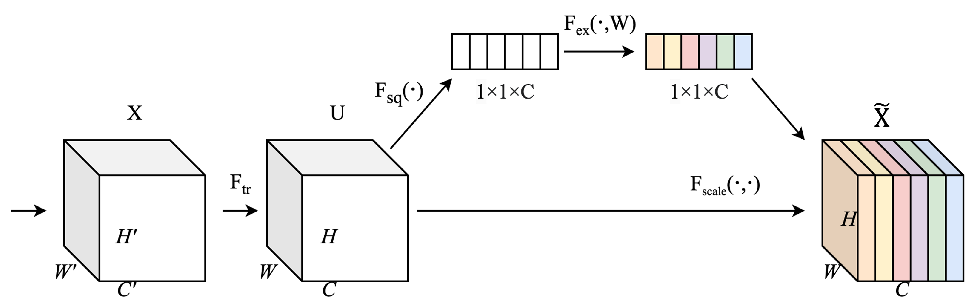
Symmetry 17 00833 g005
Figure 6. Structure of the SE module. The feature maps after excitation are shown in different colors to indicate channel-wise weighting by the SE module.
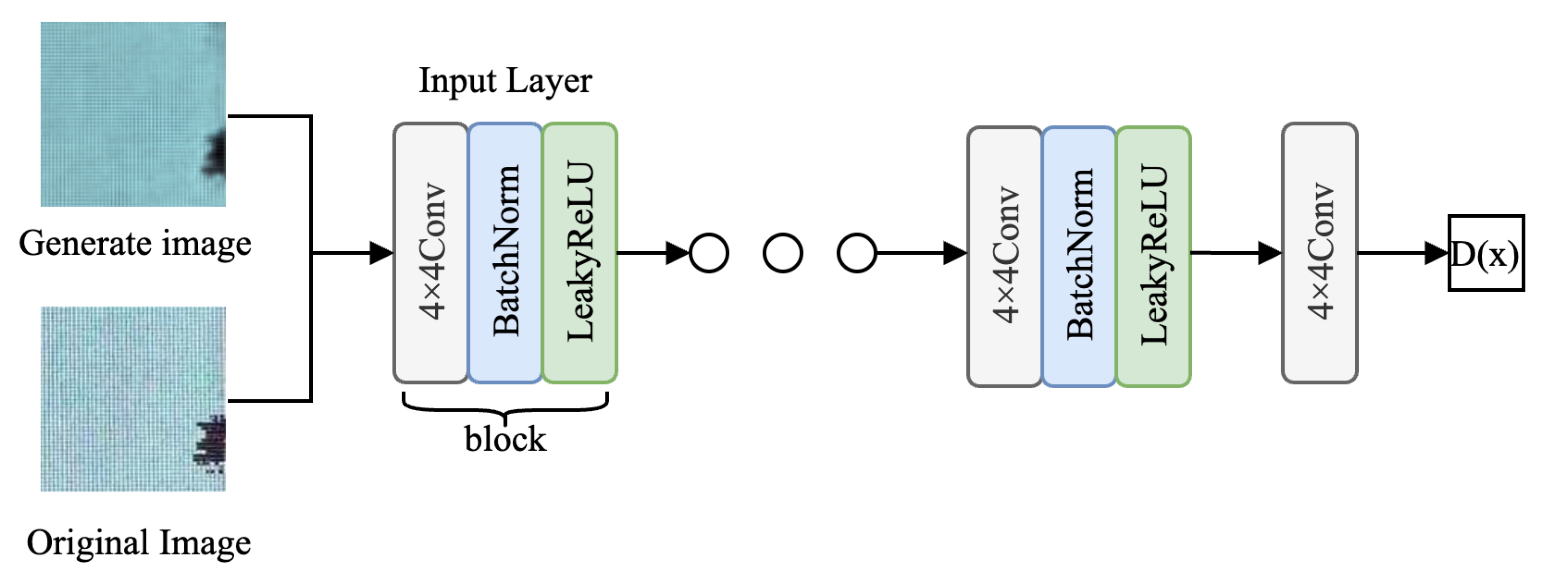
Symmetry 17 00833 g006
Figure 7. SWG-VGG discriminator structure.
Symmetry 17 00833 g007
Figure 8. Illustration of perceptual loss calculation using the VGG network. Different colors represent feature maps extracted from different layers of the VGG model.
Symmetry 17 00833 g008
Figure 9. Comparison graph of generator loss of four models.
Symmetry 17 00833 g009
Figure 10. Comparison of leakage defect images generated by four models at different training stages.
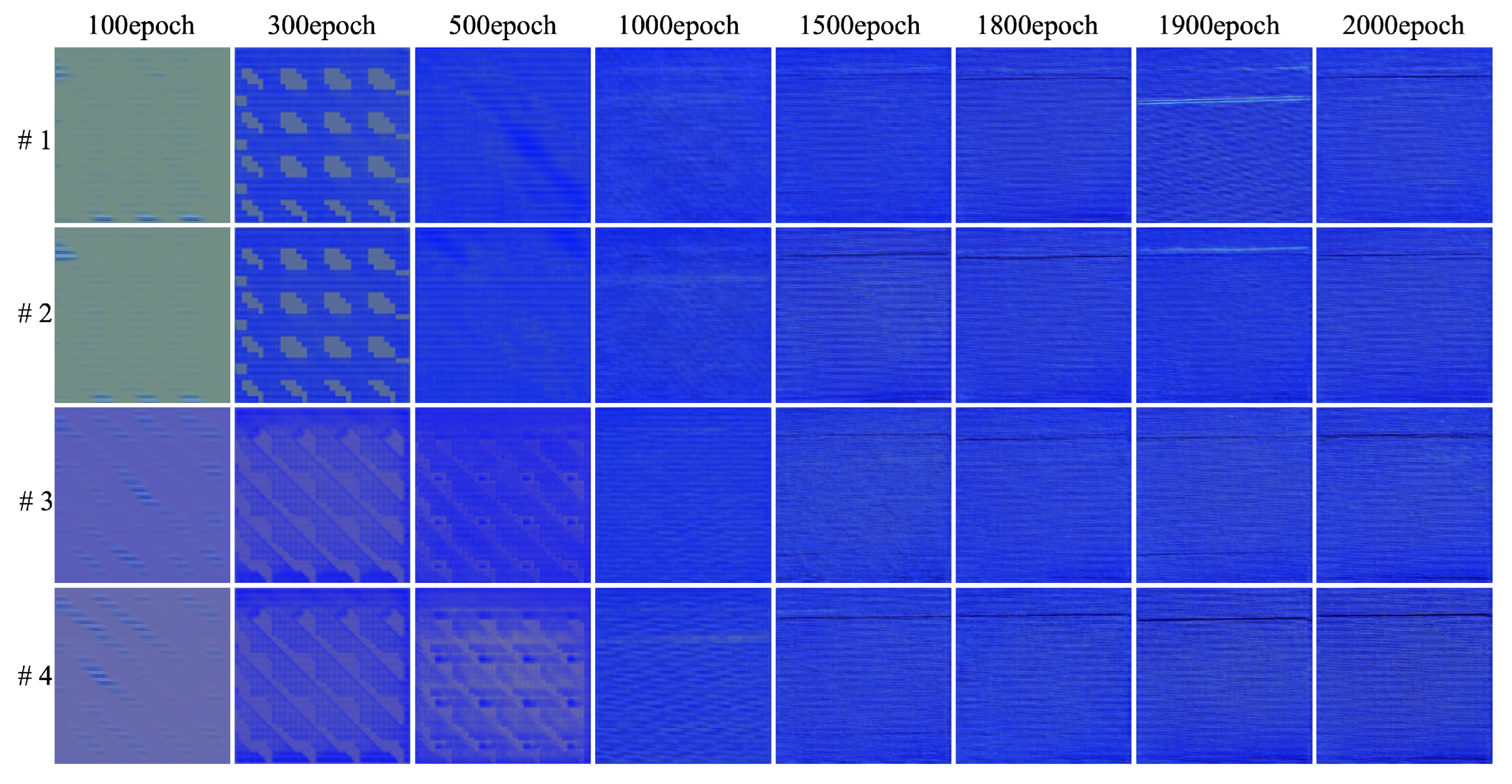
Symmetry 17 00833 g010
Figure 11. Comparison of line defect images generated by four models at different training stages. In the figure, #1, #2, #3, and #4 are Model 1, 2, 3, and 4 respectively, and 100, 300, 500, … 2000 are training rounds respectively.
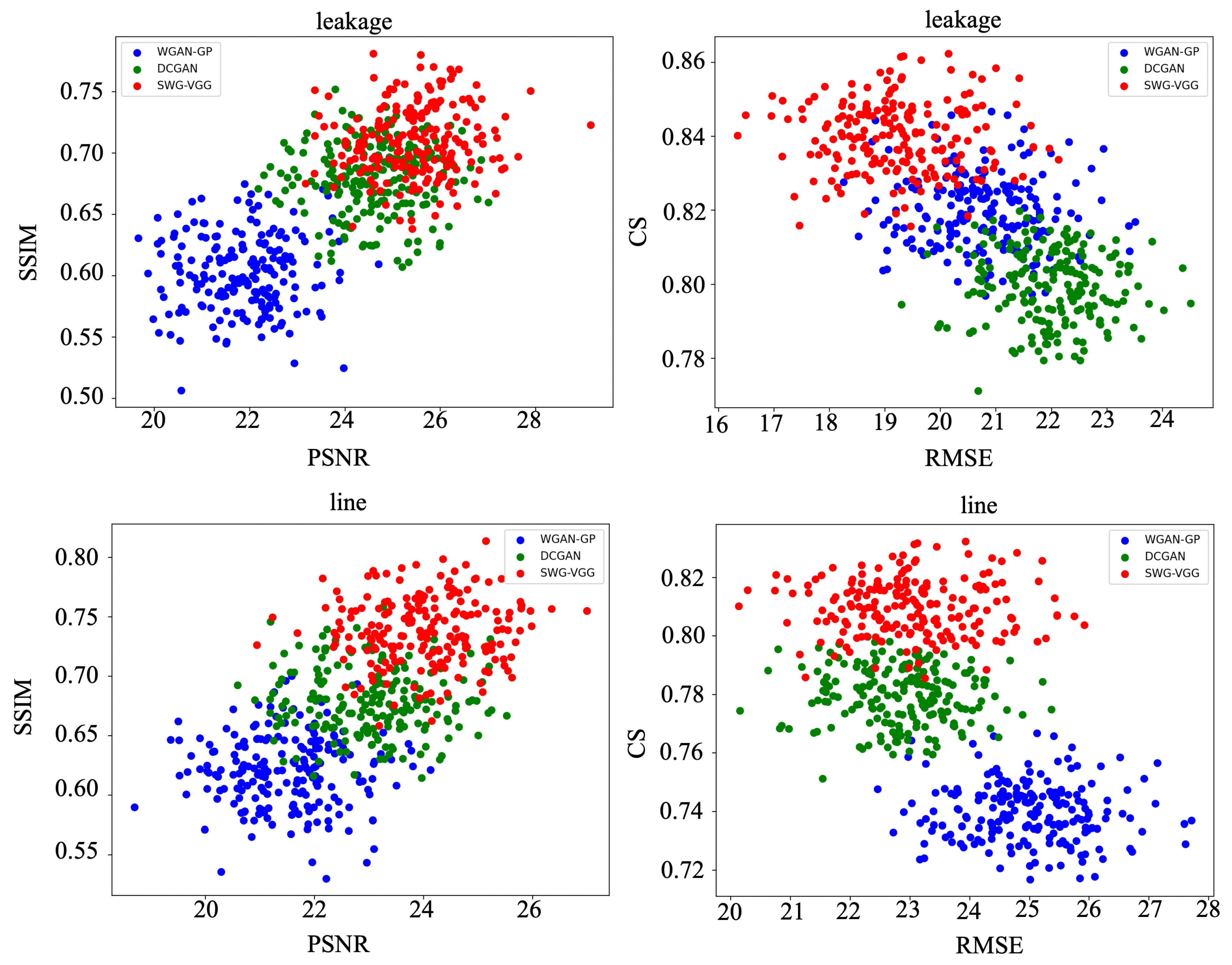
Symmetry 17 00833 g011
Figure 12. The three models randomly generate 200 images of leakage defects and line defects, and the scores of the four indicators are scatter plots.
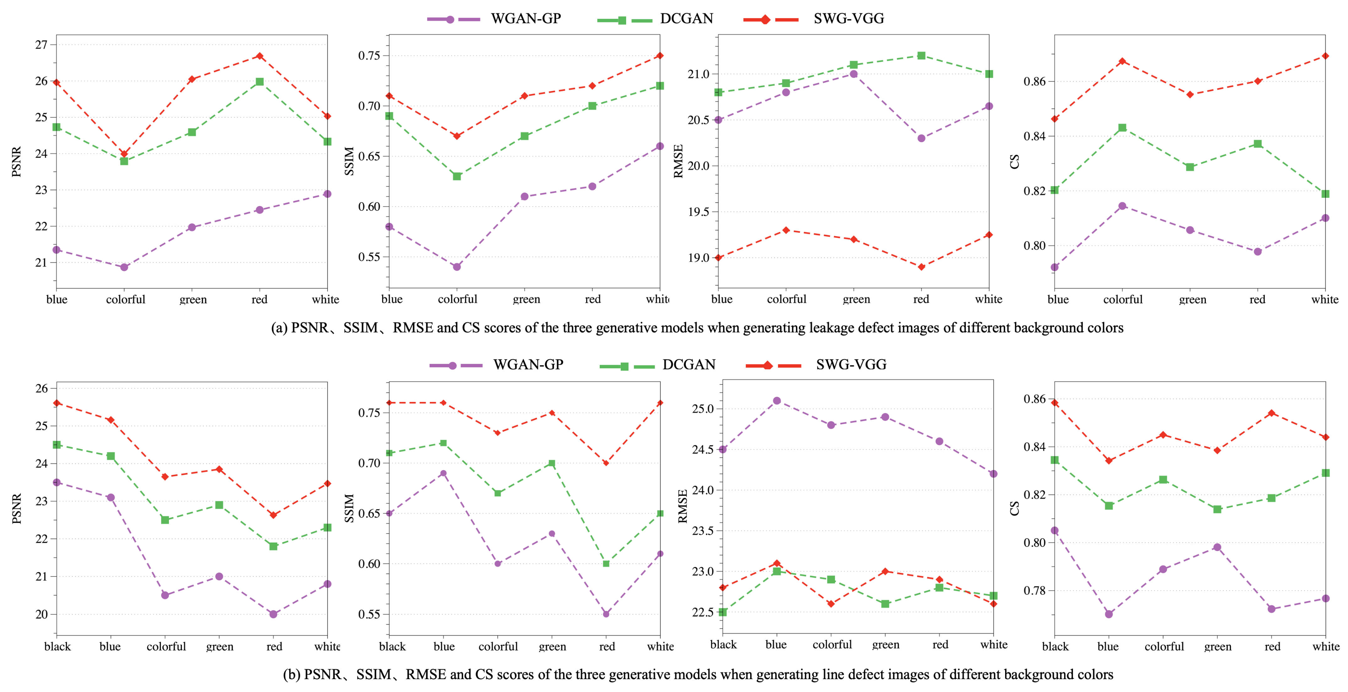
Symmetry 17 00833 g012
Figure 13. The three models randomly generate 200 images of line defects and line defects, and the scores of the four indicators are scatter plots.
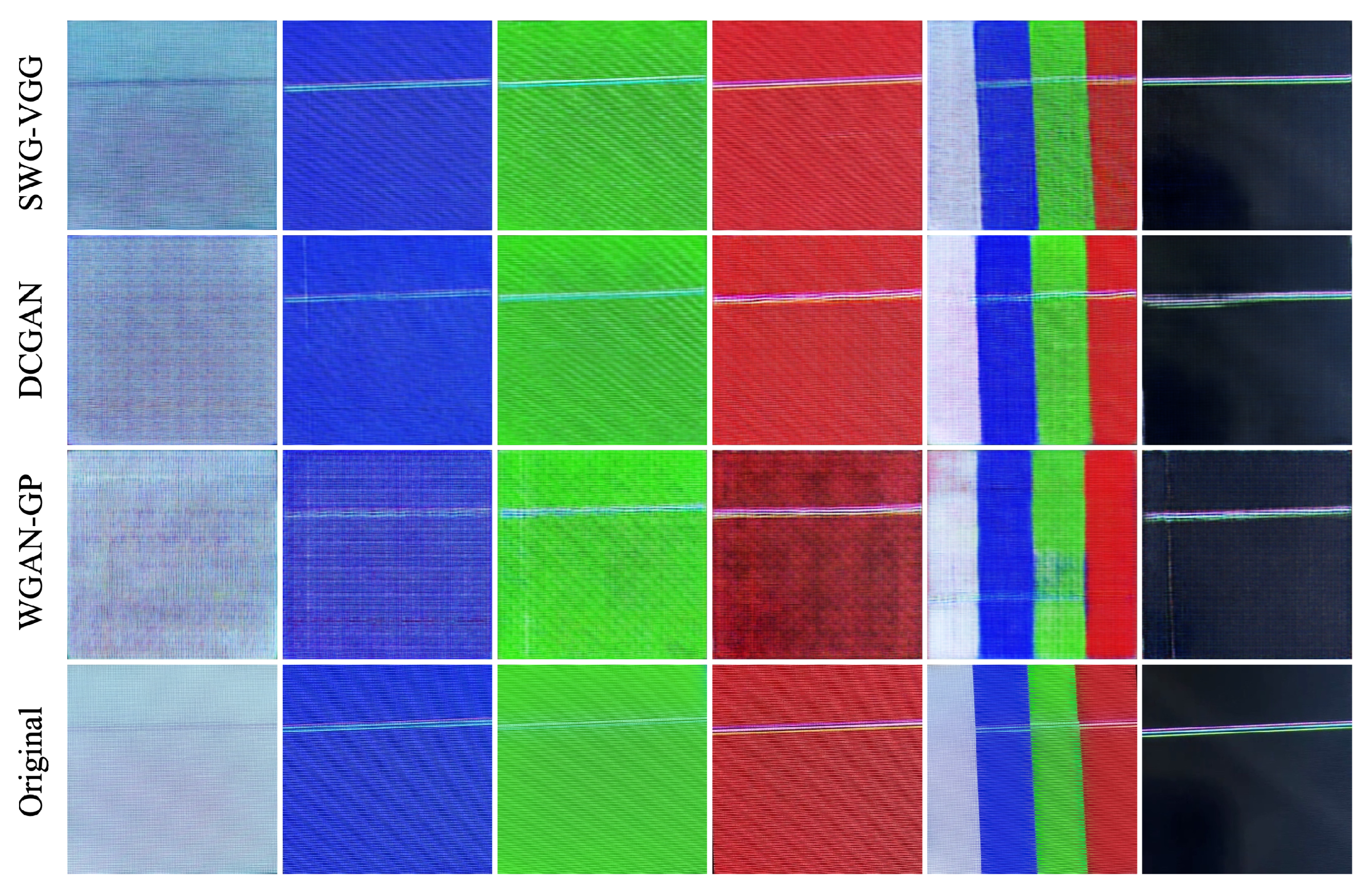
Symmetry 17 00833 g013
Figure 14. The line defect images with different background colors generated by WGAN-GP, DCGAN, and SWG-VGG models compared with the original defect images.
Symmetry 17 00833 g014
Figure 15. The leakage defect images with different background colors generated by WGAN-GP, DCGAN, and SWG-VGG models are compared with the original defect images.
Symmetry 17 00833 g015
Figure 16. Other line defects and leakage defect images generated by SWG-VGG.
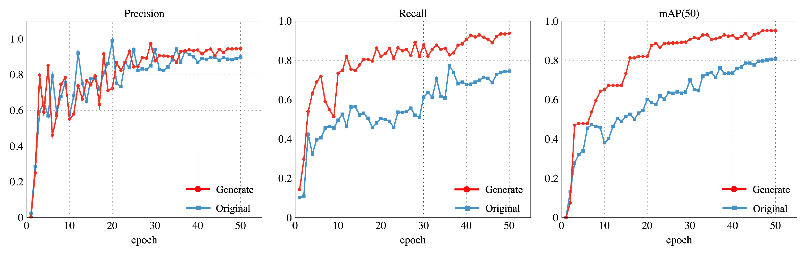
Symmetry 17 00833 g016
Figure 17. The original dataset and the enhanced dataset were used to calculate the precision, recall, and mAP@50 values.
Symmetry 17 00833 g017
Table 1. Distribution of line defect and leakage defect sample data.
ColorLineLeakage
black30-
blue3030
colorful3030
green3030
red3030
white3030
Table 2. Comparison of PSNR, SSIM, RMSE, and CS scores of four models.
ModelBasicSELpPSNRSSIMRMSECS
#1 21.960.759322.74640.7807
#2 22.530.769721.64630.7947
#3 22.350.780522.01190.7904
#423.560.801021.02260.8249
Table 3. The scores of leakage defect images generated by four models at different training stages.
IndexEpoch#1#2#3#4
PSNR10012.0012.2114.3314.30
30012.6112.2914.9615.11
50013.2810.5213.8415.15
100016.8016.3414.9415.65
150016.5218.0516.4219.44
180020.3018.2219.4922.35
190020.6220.9021.1923.42
200021.8022.8422.0823.70
SSIM1000.17980.17930.17250.1740
3000.18270.18480.17070.1894
5000.18160.16790.16080.1754
10000.18290.18850.18330.1965
15000.62170.58190.63220.7215
18000.69720.69870.71060.7926
19000.77590.78100.80460.8193
20000.78430.78350.81020.8267
RMSE10059.370055.502333.183234.3475
30054.542659.956637.161340.6640
50058.281650.940544.728841.8722
100033.546134.544141.478825.0741
150027.582924.317524.522227.4031
180023.110825.982825.598820.6448
190022.480621.831121.078119.9285
200020.646020.226420.920319.1279
CS1000.16130.23610.54230.5570
3000.54880.57030.54280.5336
5000.53640.59120.28600.3082
10000.53770.53060.48020.5647
15000.69360.62320.68060.7637
18000.76360.78870.76470.8181
19000.79440.79740.81150.8361
20000.81830.82510.82040.8447
Bold values indicate the best performance of each metric in each epoch.
Table 4. The scores of line defect images generated by four models at different training stages.
IndexEpoch#1#2#3#4
PSNR10010.3710.3215.2912.94
30017.1317.0718.3918.46
50019.2318.6919.0917.60
100018.2119.4719.0019.56
150019.9019.6420.8320.11
180020.6319.7420.6921.00
190021.1821.3421.2222.52
200022.1522.2122.5923.41
SSIM1000.11860.11670.11100.1834
3000.10710.16570.17630.1505
5000.22210.30360.39500.3577
10000.44240.49600.54720.5043
15000.56050.58190.54260.6551
18000.65940.65040.66520.7412
19000.69010.71510.71670.7743
20000.73430.75590.75080.7753
RMSE10048.481753.975247.732346.4447
30045.274745.269243.235944.8728
50041.041537.307330.868827.3125
100029.042829.152925.928726.7886
150027.399125.975725.481324.2669
180026.521625.331724.110423.5695
190024.918923.506823.405822.8818
200024.846823.066223.103422.9172
CS1000.16890.16560.12470.1397
3000.14760.28340.27200.1312
5000.34500.40240.52000.5511
10000.48900.47100.44930.4979
15000.68120.64900.66750.6512
18000.70210.71460.71930.7580
19000.73670.75170.75910.7954
20000.74300.76430.76030.8051
Bold values indicate the best performance of each metric in each epoch.
Table 5. Table of scores of defect images generated by WGAN-GP, DCGAN, and SWG-VGG models in various indicators.
WGAN-GPDCGANSWG-VGG
PSNRSSIMRMSECSPSNRSSIMRMSECSPSNRSSIMRMSECS
Leakage21.800.7820.650.8222.900.7620.900.8023.700.8319.130.84
Line22.120.7324.850.7421.960.7822.760.7823.410.7822.920.81
AV21.960.7622.750.7822.430.7721.830.7923.560.8021.020.83
Table 6. Ttable of scores of various indicators of WGAN-GP, DCGAN and SWG-VGG models in different training stages.
IndexEpochWGAN-GPDCGANSWG-VGG
PSNR10011.1813.0313.62
30014.8715.6716.78
50016.2515.5316.37
100017.5017.4317.60
150018.2118.7319.77
180020.4619.5321.67
190020.9021.1622.97
200021.9722.4323.55
SSIM1000.14920.14480.1787
3000.14490.42430.1699
5000.20180.25680.2665
10000.31260.35370.3504
15000.59110.58460.6883
18000.67830.68120.7669
19000.73300.75430.7968
20000.75930.77510.8010
RMSE10053.925847.598240.3961
30049.908646.405742.7684
50049.661540.961334.5923
100031.294432.776125.9313
150027.491025.074125.8350
180024.816225.255922.1071
190023.699722.455421.4051
200022.746421.829021.0225
CS1000.16510.26710.3483
3000.34820.41710.3324
5000.44070.44990.4296
10000.51330.48270.5313
15000.68740.65500.7074
18000.73280.74680.7880
19000.76550.77990.8157
20000.78060.79250.8249
Bold values indicate the best performance of each metric in each epoch.
Table 7. MAP@50 values of various defects in the original dataset and the dataset after adding generated images.
Original DatasetGenerate Dataset
LeakageLinePointScratchLeakageLinePointScratch
mAP@500.9410.6099629720.9950.9900.9230.995
AV0.8710.976
Table 8. Distribution of various defects in different number of datasets.
Detect
DatasetsLeakageLinePointScratch
#1train500500500500
val25252525
#2train500500500500
val25252525
#3train500500500500
val25252525
#4train500500500500
val25252525
Table 9. Statistics of each defect accuracy and average accuracy of different data sets.
DatasetsLeakageLinePointScratchAV
#10.9950.9900.9230.9950.976
#20.9940.9820.9390.9950.978
#30.9950.9800.9310.9930.975
#40.9960.9870.9540.9940.983
Disclaimer/Publisher’s Note: The statements, opinions and data contained in all publications are solely those of the individual author(s) and contributor(s) and not of MDPI and/or the editor(s). MDPI and/or the editor(s) disclaim responsibility for any injury to people or property resulting from any ideas, methods, instructions or products referred to in the content.

