Symmetric Model for Predicting Homography Matrix Between Courts in Co-Directional Multi-Frame Sequence

Abstract

The homography matrix is essential for perspective transformation across consecutive video frames. While existing methods are effective when the visual content between paired images remains largely unchanged, they rely on substantial, high-quality annotated data for a multi-frame court sequence with content variation. To address this limitation and enhance homography matrix predictions in competitive sports images, a new symmetric stacked neural network model is proposed. The model first leverages the mutual invertibility of bidirectional homography matrices to improve prediction accuracy between paired images. Secondly, by theoretically validating and leveraging the decomposability of the homography matrix, the model significantly reduces the amount of data annotation required for continuous frames within the same shooting direction. Experimental evaluations on datasets for court homography transformations in sports, such as ice hockey, basketball, and handball, show that the proposed symmetric model achieves superior accuracy in predicting homography matrices, even when only one-third of the frames are annotated. Comparisons with seven related methods further highlight the exceptional performance of the proposed model.

1. Introduction

The homography matrix is crucial for establishing coordinate mappings between paired images and plays a fundamental role in computer vision tasks such as camera calibration [1,2], image stitching [3,4], illumination estimation [5,6], and simultaneous localization and mapping [7]. Similarly, in team ball sports competitions, the homography matrix is used to transform the players’ positions from a live TV perspective to a standardized top view. This transformation enables the calculation of metrics such as movement speed, acceleration, and running distance, facilitating a quantitative assessment of player performance.

Directly converting a competitive video frame to a standardized top view, as shown in Figure 1a, is often challenging due to the significant difference between the live TV perspective and the standardized top view, given the constant movement of the content on screen. Therefore, as shown in Figure 1b, the primary focus is typically on studying the homography transformation between consecutive frames and then indirectly achieving the goal by manually annotating the transformation parameters $H_{manual}$ of a frame to the standardized top view image.

Research on homography matrix prediction initially relies on significant feature points in images to establish the mapping relationship [8,9,10]. Follow-up studies propose extracting lines and curves [11,12,13], which could also incorporate color information [14] and shape features [15]. Although these methods yield favorable results, the task of matching line segments in images still requires further optimization [16]. To improve both feature extraction and matching, convolutional neural network (CNN) is extensively researched [17,18]. The network overcomes the limitations of finite points or line segments and significantly enhances robustness, but it comes with the drawback of requiring extensive data annotation. When directly applied to the vast number of frames in competitive sports videos, the accuracy of homography matrix prediction decreases significantly. The intense competition among players and continuous camera movements further diminish the performance of these methods.

To overcome the limitations of existing methods for predicting homography matrices within frame sequence, we draw inspiration from the bidirectional recurrent neural network (RNN) [19], the mutual invertibility property of homography matrices, HomegraphyNet [18], and the codirectional shooting characteristics of team ball competition videos to propose a model that introduces a symmetric bidirectional stacked neural network. This model predicts continuous homography matrices between courts in a co-directional frame sequence, requiring just a few data annotations during training. This study makes three key contributions:

• The model exploits the mutual invertibility property of bidirectional homography transformation matrices for paired images, enhancing the accuracy of homography transformation even in scenarios with certain content changes.
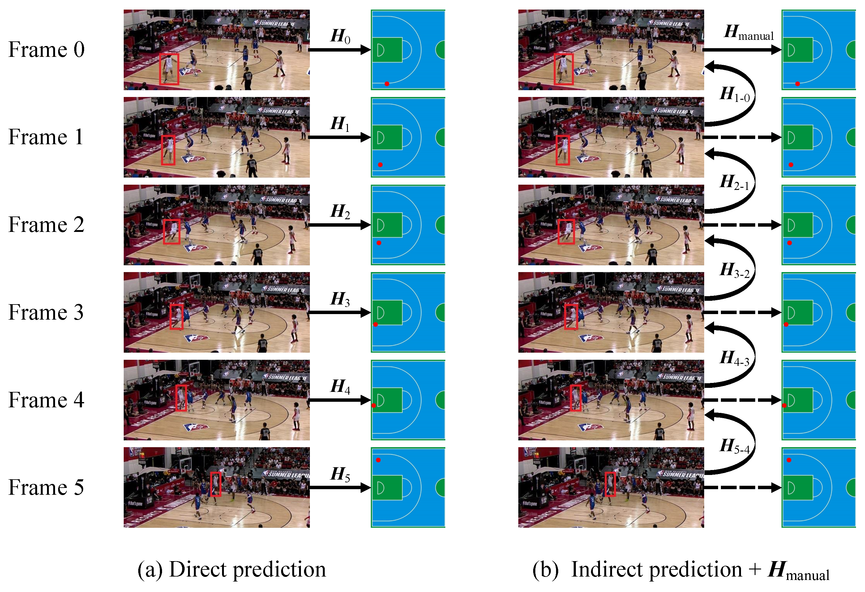
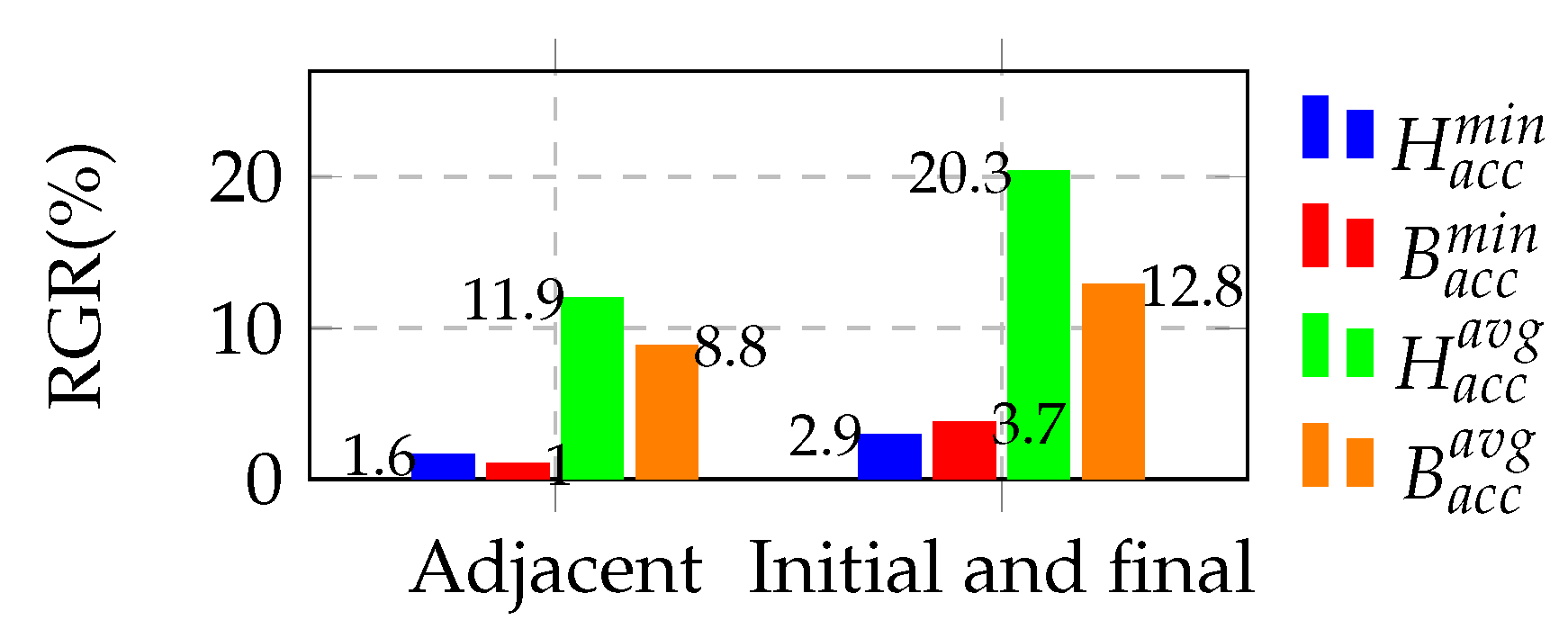
• By leveraging matrix decomposition, the proposed method requires homography matrix annotation only for the initial and final frames, thereby reducing the data annotation workload.
• The proposed strategy of selecting four pairs of keypoints effectively trains the symmetric bidirectional stacked neural network by using a continuous frame sequence as input.

2. Related Work

Homography Transformation Based on Displayed Features. Traditional approaches for predicting homography matrix between paired images rely on selected matching elements that effectively represent the uniqueness of their features. Specifically, a typical method is to obtain corner points using the Harris detector [20], although it is sensitive to scale changes. The SIFT (Scale Invariant Feature Transform) detector [21,22] improves by being invariant to rotation changes. Other keypoint detectors, such as the ORB (Oriented FAST and Rotated BRIEF) detector [23], SURF (Speeded Up Robust Feature) detector [24], and LBP (Local Binary Patterns) detector [17], are also available. However, due to the continuous movement of players wearing similar kits and the large areas of similarity on the court, homography transformation based on these points may not yield optimal results. To address these challenges, researchers have proposed improved methods to obtain more effective mapping information. Yao et al. [25] extracted distinctive T-shaped intersections on the court and combined them with the direct linear transformation algorithm or with the video mosaic calibration algorithm based on line segment features for matching. Doria et al. [26] utilized color for image segmentation and extracted court boundary line segments [14,27] to perform inter-court homography transformation. However, these methods only provide local information and do not fully capture the target subjects. Moreover, the constantly changing video shooting perspective can exacerbate the failure of transformation. Thus, Liu et al. [9] attempted to incorporate video shooting angles into the line segment matching process, while Lao et al. [28] proposed a method of inter-court homography transformation that relies on kinematics models. Nonetheless, these methods offer limited improvements for team sports with rapid player movement and complex interactions. In summary, methods of predicting homography matrix based on display features are not suitable for competitive sports with constantly changing visual content, and the separation of feature extraction and matching steps may also introduce additional errors.

Homography Transformation Based on Deep Learning. In recent years, research on homography transformation among paired images has focused on enhancing deep learning networks that integrate feature extraction and matching processes. One of the early studies is HomographyNet [18], proposed by DeTone et al. This model generates data annotations by utilizing the positional deviation of 4 randomly selected keypoints before and after homography transformation of the same content image, demonstrating the feasibility of end-to-end deep learning for homography transformation. Subsequently, Wang et al. [29] incorporated a pyramid structure into the network to improve feature extraction effectiveness. Since homography transformation requires two related images as input, Czolbe et al. [30] enhanced the single-branch CNN used in HomographyNet by developing a double-branch approach. Ghassab et al. [31] applied an enhanced version of HomographyNet for homography transformation among paired images of courts; however, the use of Mask R-CNN to identify and exclude regions containing player regions may introduce instability. Moreover, researchers have explored using color blocks to improve homography transformation within deep neural networks. For instance, Molina-Cabello et al. [32] proposed a refinement operation based on color blocks, which generates tentative color transformations from paired images to improve the accuracy of the homography matrix. Similarly, CNN models based on similar block features have been employed for homography transformation by Zeng et al. [33]. Photometric information has also been recognized as an important feature that can enhance homography transformation, as demonstrated by Wang et al. [34] and Kang et al. [6], who incorporated photometric error into the loss function to improve accuracy. However, acquiring color, similar blocks, and luminosity can be influenced by local self-similar features, posing challenges when directly applied to scenes with a large number of similarly dressed players and a uniformly colored court, which are the focus of this paper. Both supervised and weakly supervised deep learning models require extensive data annotation to improve homography transformation between paired images with content changes, further constraining the development of relevant methods in competitive sports [35,36]. Therefore, self-supervised and unsupervised learning methods have become a recent research focus. Almost all related advancements use spatial transformer networks combined with model-predicted homography matrices to perform homography mapping on each pixel in standardized images, driving the training of overall network parameters. Researchers such as Nguyen et al. [37], Wang et al. [38], and Koguciuk et al. [39] have adopted this approach and incorporated optical flow loss. However, these methods rely on the basic assumption that the original image should align with the target image after homography transformation. This assumption becomes ineffective when the content of paired images changes. Additionally, Jiang et al. [40] proposed a semi-supervised network for homography matrix prediction of sequential images, which inserts more images between labeled image pairs. Although these images lack training labels, the product of the homography matrices among consecutive image pairs is exactly equal to the homography matrix between the first and last frames, thus reducing the need for data labels. However, the number of inserted images in this method is a hyperparameter that significantly impacts the stability of the model.

3. Methods

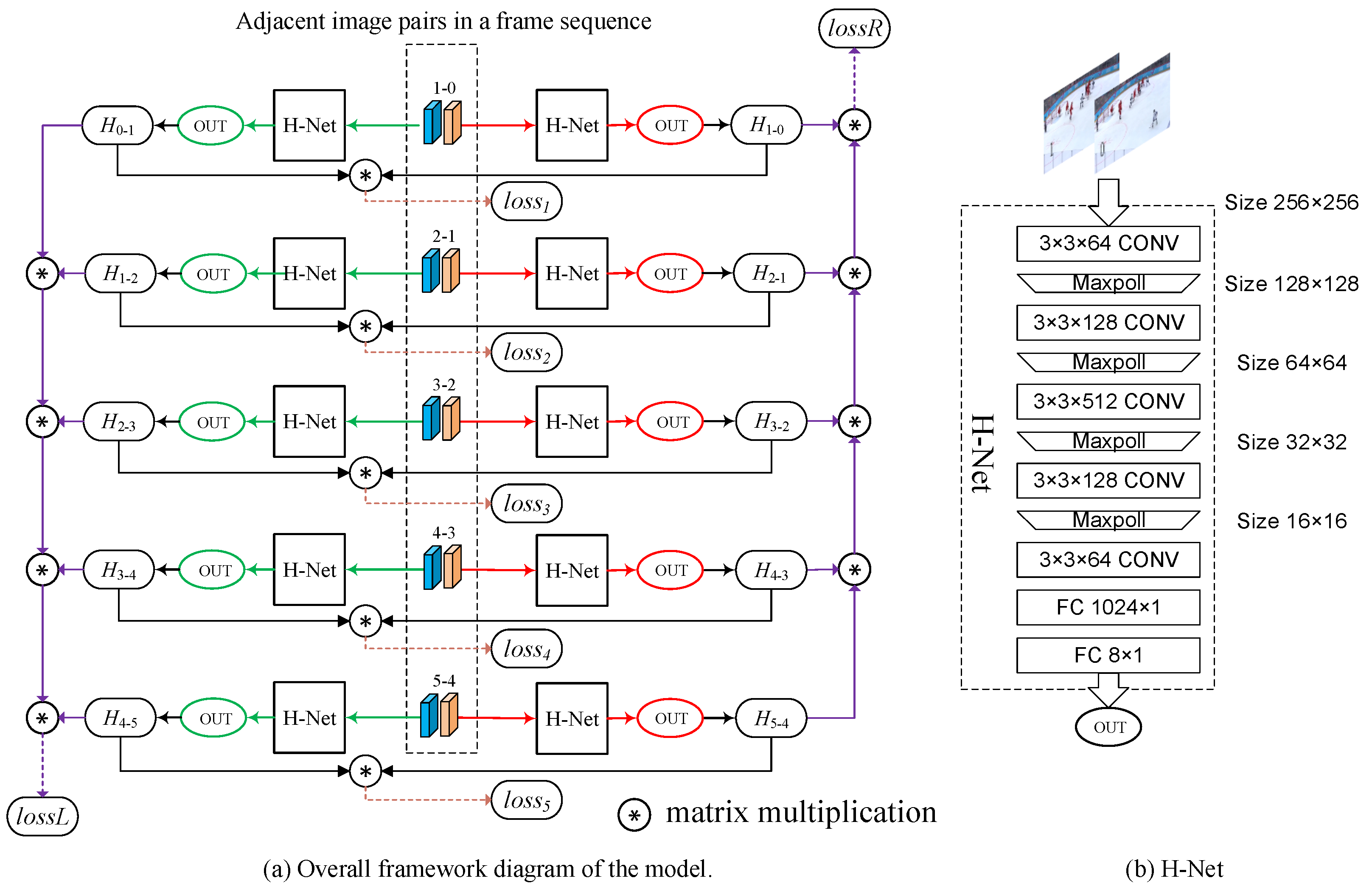
3.1. Overall Architecture

This paper presents a homography matrix prediction model for court transformations. Overall, the symmetric model, illustrated in Figure 2, consists of five repeated structures and forms a bidirectional stacked neural network.

The model is based on two key theoretical principles from matrix theory: the decomposability of homography matrices and the fact that a matrix multiplied by its reciprocal yields the identity matrix. This means that the homography matrix between the initial and final frames of a sequence can be decomposed into the product of five intermediate matrices. These intermediate matrices correspond to the homographies between adjacent paired images, transforming a complex one-step prediction into a more manageable five-step process, thereby reducing the data annotation burden. Each of these repetitive structures consists of two identical H-Net modules, which facilitates the use of bidirectional homography matrix invertibility. This design also helps mitigate the impact of visual content changes between images, reducing potential errors introduced by treating intermediate matrices as ground truth labels. Additionally, within H-Net, we have innovatively designed a strategy for selecting four keypoints that are specifically suited for predicting homography matrices in sequence images based on theoretical calculations. Further details of this approach are provided in the following section.

3.2. Decomposability of Homography Matrix

The decomposability of the homography matrix constrains the overall structure of the model and reduces the amount of data annotation required for training.

Equation (1) represents the fundamental formula for the homography transformation between paired images.

$${\mathit{H}}_{s\to t}·{\overrightarrow{\mathit{L}}}_s={\overrightarrow{\mathit{L}}}_t$$

(1)

It incorporates the pixel position ${\overrightarrow{\mathit{L}}}_s$ in the source image, the corresponding pixel position ${\overrightarrow{\mathit{L}}}_t$ in the target image, and the homography matrix ${\mathit{H}}_{s\to t}$ required to transform positions from the source perspective to the target perspective, as defined in Equation (2).

$${\mathit{H}}_{s\to t}=\left[\begin{array}{ccc}{h}_0& h_1& h_2\\ h_3& h_4& h_5\\ h_6& h_7& 1\end{array}\right]$$

(2)

where $h_0$ to $h_7$ respectively represent the 8 degrees of freedom of the homography matrix. $s\to t$ represents the homography transformation performed from the perspective of the source image s to the perspective of the target image t.

Assume a sequence of n consecutive frame images is randomly sampled from a competitive sports video captured with a consistent camera movement direction. The homography matrices between each adjacent paired image are then computed using the basic homography transformation formula, as illustrated in Equation (3). Subsequently, the source perspective pixel points in the current paired images are substituted with the target perspective pixel points from the previous paired images, resulting in the final output presented in Equation (4). Furthermore, the homography transformation between the initial and final frames of the sequence can be expressed by Equation (5). By comparing Equation (4) with Equation (5), Equation (6) is derived, demonstrating that for a sequence composed of multiple frames, the homography transformation matrix between the initial and final frames can be decomposed into the product of the homography matrices between adjacent paired images throughout the sequence. Therefore, the model can predict the homography matrix ${\mathit{H}}_{0\to n-1}$ when transforming from frame 0 to frame $n-1$.

$$\begin{array}{cc}\hfill {\mathit{H}}_{n-2\to n-1}·& {\overrightarrow{\mathit{L}}}_{n-2}={\overrightarrow{\mathit{L}}}_{n-1}\hfill \\ \hfill {\mathit{H}}_{n-3\to n-2}·& {\overrightarrow{\mathit{L}}}_{n-3}={\overrightarrow{\mathit{L}}}_{n-2}\hfill \\ \hfill & \dots \hfill \\ \hfill {\mathit{H}}_{1\to 2}·& {\overrightarrow{\mathit{L}}}_1={\overrightarrow{\mathit{L}}}_2\hfill \\ \hfill {\mathit{H}}_{0\to 1}·& {\overrightarrow{\mathit{L}}}_0={\overrightarrow{\mathit{L}}}_1\hfill \end{array}$$

(3)

$${\mathit{H}}_{n-2\to n-1}·{\mathit{H}}_{n-3\to n-2}\dots \dots {\mathit{H}}_{0\to 1}·{\overrightarrow{\mathit{L}}}_0={\overrightarrow{\mathit{L}}}_{n-1}$$

(4)

$${\mathit{H}}_{0\to n-1}·{\overrightarrow{\mathit{L}}}_0={\overrightarrow{\mathit{L}}}_{n-1}$$

(5)

$${\mathit{H}}_{0\to n-1}={\mathit{H}}_{n-2\to n-1}·{\mathit{H}}_{n-3\to n-2}\dots \dots {\mathit{H}}_{0\to 1}$$

(6)

Given the bidirectional nature of homography transformation among paired images, we can incorporate the decomposability of the homography matrix between the final and initial frames in the reverse direction by combining Equation (6) with the structure illustrated in Figure 1. This enables us to establish the matrix relationship expressed in Equation (7), which is used to express the homography matrix ${\mathit{H}}_{n-1\to 0}$ when the model predicts the transformation from frame n-1 to frame 0.

$${\mathit{H}}_{n-1\to 0}={\mathit{H}}_{1\to 0}\dots \dots {\mathit{H}}_{n-2\to n-3}·{\mathit{H}}_{n-1\to n-2}$$

(7)

By considering the decomposability of the homography matrix described by Equations (6) and (7) as a constraint condition, we formulate the loss function represented in Equation (8) using the L1-norm with the homography matrix ground truth annotations ${\mathit{H}}_{begin\to end}$ and ${\mathit{H}}_{end\to begin}$, which are defined between the initial and final frames of the sequence.

$$\begin{array}{cc}\hfill lossRL& =lossR+lossL\hfill \\ & =\sum _{k=0}^8\mid {\mathit{H}}_{begin\to end}\left[k\right]-{\mathit{H}}_{0\to n-1}\left[k\right]\mid +\mid {\mathit{H}}_{end\to begin}\left[k\right]-{\mathit{H}}_{n-1\to 0}\left[k\right]\mid \hfill \end{array}$$

(8)

where $lossR$ and $lossL$ represent the loss functions calculated in each direction, and $k\in \{0,1,2,3,4,5,6,7\}$ represents the element index of the homography matrix.

Based on the above principle, if the sequence length n of a single input to the model is set to 5, only the labels required for homography transformation between frames 0 and 5, as well as between frames 5 and 0, need to be labeled. So, there is no need to label homography transformation labels between paired images such as 0-1, 1-2, 2-3, 3-4, and 4-5 using traditional methods. As a result, the amount of data annotation is reduced to at least one-third of the original.

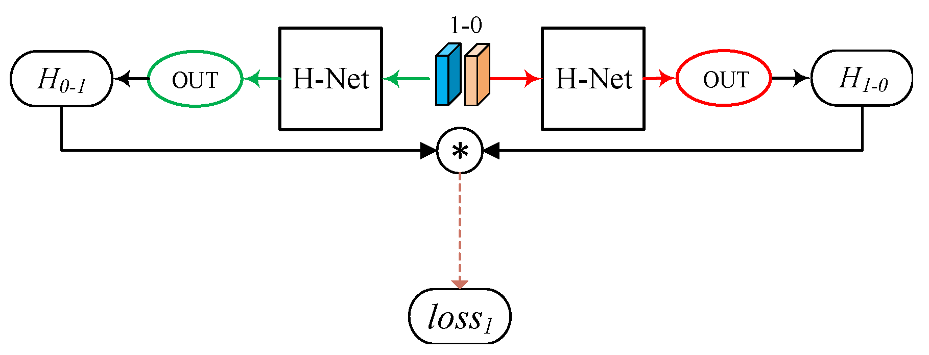
3.3. Mutual Invertibility of Bidirectional Homography Matrices

The mutual invertibility of bidirectional homography matrices enhances the model’s training performance for paired images with changing content without requiring additional data labels.

Assume a pair of images with frames numbered n and n + 1. Two separate homography transformations are executed: one is the transformation from image n to image n + 1, and the other is the reverse transformation. The corresponding transformation relations are depicted in Equations (9) and (10), respectively.

$${\mathit{H}}_{n\to n+1}·{\overrightarrow{\mathit{L}}}_n={\overrightarrow{\mathit{L}}}_{n+1}$$

(9)

$${\mathit{H}}_{n+1\to n}·{\overrightarrow{\mathit{L}}}_{n+1}={\overrightarrow{\mathit{L}}}_n$$

(10)

By substituting Equation (9) into Equation (10), Equation (11) can be obtained based on the uniqueness of the paired images.

$${\mathit{H}}_{n\to n+1}·{\mathit{H}}_{n+1\to n}=\mathit{E}$$

(11)

Similarly, by substituting Equation (10) into Equation (9), Equation (12) can be derived.

$${\mathit{H}}_{n+1\to n}·{\mathit{H}}_{n\to n+1}=\mathit{E}$$

(12)

Hence, it can be demonstrated that, under ideal conditions, the homography matrices predicted from both directions of the same pair of images are mutually inverse.

Thus, by leveraging the mutual invertibility of the bidirectional homography matrix, as illustrated in Figure 2, the overall framework adopts the same network to achieve the corresponding homography transformation from two reverse directions within a single run of the stacked unit. The L1 norm is applied in the loss function, as presented in Equation (13), to enhance precision, particularly when there are substantial content variations among inter-frame images without introducing additional manual data annotation. 

$$los{s}_i=\sum _{k=0}^8\mid {\mathbf{e}}_i\left[k\right]-\mathbf{E}\left[k\right]\mid$$

(13)

Here, i represents the i-th stacked unit, $\mathit{e}$ and $\mathit{E}$ are 3 × 3 matrices, with the former being the product of homography matrices from bidirectional predictions and the latter being the identity matrix, where k represents the matrix element index.

Essentially, the unit depicted in Figure 3 encompasses only a single pathway, where H-Net denotes the network, and OUT represents the positional deviation of 4 specific keypoints. This unit employs images numbered 0 and 1 to form paired images 0-1 and paired images 1-0 for bidirectional homography transformation.

At this point, it is important to note that although Equation (13) constrains the mutual homography transformation process between paired images. However, it does not guarantee that the predicted homography matrix closely approximates the true homography matrix. Therefore, process corrections are implemented from two key aspects.  Firstly, as described in subsequent experiments, extensive pre-training is conducted on H-Net using paired images with identical content. This step initially minimizes the deviation in the homography matrix predicted between paired images with varying content. Secondly, by leveraging the decomposability of the homography matrix, the parameters of the five H-Nets are averaged after each round of training. This averaging further ensures that the prediction results, under the mutual invertibility constraint of the homography matrix, converge to a unique and correct solution.

When the model processes a sequence consisting of p frames simultaneously, the loss function in Equation (14) is computed. Here, $lossM$ represents the loss function derived from the mutual invertibility property of the bidirectional homography matrices for all paired images.

$$lossM=\sum _{i=0}^{p-1}los{s}_i$$

(14)

3.4. Key Point Selection Strategy

The stacked unit illustrated in Figure 3 is an enhanced version of HomographyNet, with the primary improvement being the development of a dedicated strategy for computing the homography matrix. This enhancement enables the use of sequence images consisting of three or more frames for model training rather than being limited to only two frames.

In the original HomographyNet, the positional deviation of 4 keypoints before and after the transformation of the paired images served as data labels. These paired images consist of an input image and another image generated by applying a random homography transformation to the input image, as shown in Figure 4a. However, in the co-directional frame sequence addressed in this paper, only the homography matrix mapping between the initial and final frames is available, with limited mapping information for other paired images. This limitation prevents the random selection of keypoints in the middle paired images for prediction, making it impossible to train the network to express the decomposability of the homography matrix.

To address this, 4 specific keypoints are selected for the paired images, as shown in Figure 4b. This strategy fixes the 4 corners of an image as keypoints, with the model predicting the positional deviation before and after the homography transformation for each key point.

$$\left[\begin{array}{cccccccc}0& 0& 1& 0& 0& 0& 0& 0\\ 0& 0& 0& 0& 0& 1& 0& 0\\ a& 0& 1& 0& 0& 0& -a(a+{\delta }_2)& 0\\ 0& 0& 0& a& 0& 1& -a{\delta }_3& 0\\ 0& b& 1& 0& 0& 0& 0& -b{\delta }_4\\ 0& 0& 0& 0& b& 1& 0& -b(b+{\delta }_5)\\ a& b& 1& 0& 0& 0& -a(a+{\delta }_6)& -b(a+{\delta }_6)\\ 0& 0& 0& a& b& 1& -a(b+{\delta }_7)& -b(b+{\delta }_7)\end{array}\right]\times \left[\begin{array}{c}{h}_0\\ h_1\\ h_2\\ h_3\\ h_4\\ h_5\\ h_6\\ h_7\end{array}\right]=\left[\begin{array}{c}{\delta }_0\\ {\delta }_1\\ a+{\delta }_2\\ {\delta }_3\\ {\delta }_4\\ b+{\delta }_5\\ a+{\delta }_6\\ b+{\delta }_7\end{array}\right]$$

(15)

Specifically, for an input image with effective pixel dimensions a (length) and b (width), the 4 keypoints are located at coordinates (0, 0), (a, 0), (0, b), and (a, b). The homography transformation equation, Equation (15), is derived from Equation (1) using the positional deviations of each pixel after transformation. The positional deviation of the (0, 0) pixel in the input image after transformation into the target image is (${\delta }_0$, ${\delta }_1$); for the (a, 0) pixel, it is (${\delta }_2$, ${\delta }_3$); for the (0, b) pixel, it is (${\delta }_4$, ${\delta }_5$); and for the (a, b) pixel, it is (${\delta }_6$, ${\delta }_7$). The homography matrix $\mathit{H}$ for the paired images is then generated, with each matrix element detailed in Appendix A. This strategy enables the bidirectional stacked neural network to effectively express the decomposability properties of the homography matrix.

4. Experimental Setup

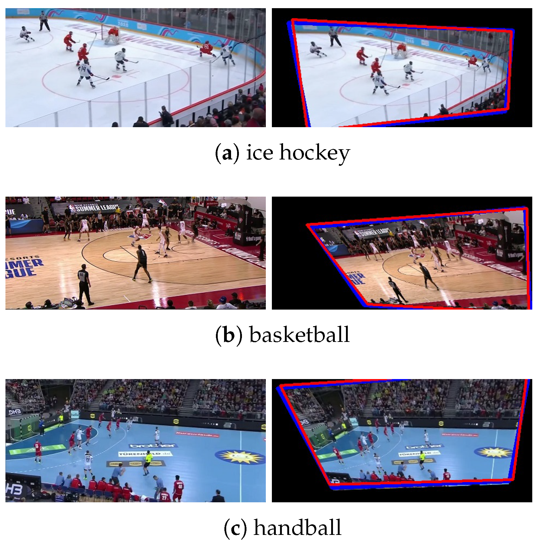
4.1. Experimental Environment and Dataset

All experiments are conducted on an NVIDIA A100 GPU using PyTorch 1.5. The dataset for homography matrix prediction comprised 12,000, 9600, and 12,000 groups of co-directional frame sequence from ice hockey [41], basketball [42], and handball [43] competitive videos, respectively. Each group contains six consecutive images randomly selected from live broadcasts. While homography matrices are manually annotated for all adjacent paired images, only the matrix between the initial and final frames was used for model training.

4.2. Pre-Training of the Stacked Unit Network

Due to the fixed coordinate positions of certain keypoints, and by referencing the unsupervised learning dataset generation method in HomographyNet, our approach automatically constructs a pre-training dataset of paired images with identical visual content, eliminating the need for additional data annotation. The pre-training dataset included 60,000 ice hockey paired images, 48,000 basketball paired images, and 60,000 handball paired images.

Before being input into the stacked units, each image is resized to 256 × 256 pixels. Stochastic Gradient Descent (SGD) with a momentum of 0.9 and an initial learning rate of 0.01 is employed, with the learning rate reduced by a factor of 10 every 10,000 iterations. The detailed structure of the unit network is shown in Figure 2b. Training is conducted for 40,000 iterations for ice hockey, 32,000 iterations for basketball, and 40,000 iterations for handball, with a batch size of 64.

The visualization results of the homography transformation pre-training are shown in Figure 5. The source perspective is indicated by the blue box, while the target perspective is represented by the red box. The degree of overlap between the blue and red boxes in the target image (the right image in each pair) reflects the accuracy of the homography transformation. Analysis confirms that, after pre-training, the stacked unit network accurately predicts the homography matrix for input paired images with identical visual content.

4.3. Performance Metrics

Due to the inherent errors in manually labeling a substantial number of paired images, we develop a new metric for quantifying prediction accuracy. Inspired by Equation (16) in Refs. [44,45], this metric assesses the disparity between the predicted pixel point position ($x_p$, $y_p$) and the theoretically annotated pixel point position ($x_l$, $y_l$). Specifically, a pixel pair is considered a successful match if the Euclidean Distance Point Error (PE) between them is within 16 pixels, incrementing ${\mathit{H}}_{tp}$. Conversely, an unsuccessful match increments ${\mathit{H}}_{fn}$. Combined with the Average Correspondence Error (ACE), this forms the calculation method for the new metric, as shown in Equation (17).

$$PE=\sqrt{{\displaystyle \frac{1}{4}}·\sum _{i=1}^4((x_p^i-x_l^i)+(y_p^i-y_l^i))}$$

(16)

$${\mathit{H}}_{acc}={\displaystyle \frac{{\mathit{H}}_{tp}}{{\mathit{H}}_{tp}+{\mathit{H}}_{fn}}}$$

(17)

Simultaneously, drawing inspiration from the Intersection over Union (IoU) metric and incorporating the Mean Intersection over Union (MIoU) calculation method from Ref. [33], we devise another method to quantify the matching degree of block regions between the predicted block ${\mathit{S}}_p$ and the annotated block ${\mathit{S}}_l$, as outlined in Equation (18). Given that player movement inevitably introduces both matching and non-matching blocks in paired images, we assess the effectiveness of block matching by calculating the Block Intersection over Union (BIoU). A BIoU value exceeding 0.5 indicates successful block matching, incrementing ${\mathit{B}}_{tp}$. Conversely, invalid block matching increments ${\mathit{B}}_{fn}$. If an unmatched block generates a matching output, the block matching is considered invalid, leading to an increment in ${\mathit{B}}_{fp}$. The calculation method for this metric, which integrates Equation (18) and the block matching algorithm from Refs. [44,46], is demonstrated in Equation (19).

$$BIoU={\displaystyle \frac{{\mathit{S}}_p\cap {\mathit{S}}_l}{{\mathit{S}}_p\cup {\mathit{S}}_l}}$$

(18)

$${\mathit{B}}_{acc}={\displaystyle \frac{{\mathit{B}}_{tp}}{{\mathit{B}}_{tp}+{\mathit{B}}_{fn}+{\mathit{B}}_{fp}}}$$

(19)

5. Results and Discussion

5.1. Stacking Quantity Selection Experiment

Considering the need for real-time processing, we conduct further experiments on selecting the number of stacked units in our model using a combined dataset of three types of competitive sports images. These experiments help clarify the rationale behind the overall model architecture. The results are summarized in

Table 1. Stacking quantity selection experiment results.

Quantity	Parameters	Time (ms)	Proportion of Labels (%)	${\mathit{H}}_{\mathit{acc}}(\%)$	${\mathit{B}}_{\mathit{acc}}(\%)$
2	67 M	31.3	50	88.2	90.4
3	84 M	47.8	33.3	86.6	88.5
4	100 M	64.6	25	84.9	86.3
5	117 M	80.4	20	83.8	85.7
6	134 M	96.1	16.7	71.4	74.6
7	151 M	112.5	14.3	48.7	55.3

. The evaluation metrics include the number of parameters, time consumption, proportion of data labeling required, and $H_{acc}$ and $B_{acc}$ between the initial and final frames. The proportion of data labeling required is defined as the reciprocal of the number of image pairs that can be effectively utilized with a single manual annotation, thus indicating the model’s dependence on manual data labeling. For example, if one image pair requires only one label, the proportion is 1. The results indicate that models with fewer stacked units tend to achieve better performance but require a higher number of manual labels. Furthermore, it is observed that the model performs best with a maximum of five stacked units. When the number exceeds five (i.e., six or more), model performance deteriorates significantly. Based on this analysis, we ultimately select a stacking quantity of five for our proposed framework.

5.2. Ablation Experiment

To comprehensively analyze the contributions of bidirectional homography matrix invertibility and homography matrix decomposability within sequential frames, we design three distinct experimental schemes and conduct ablation studies on the dataset. The results demonstrate that the mutual invertibility of bidirectional homography matrices is critical for accurately processing individual paired images, while the decomposition of the homography matrix significantly enhances the model’s capability to handle entire image sequences.

Specifically, in scheme one, only the mutual invertibility of the bidirectional homography transformation matrices is utilized—meaning the model is trained using only the loss function $lossM$. Scheme two focuses solely on its decomposability, with training based only on the loss function $LossRL$. Scheme three combines both properties and incorporates both $lossM$ and $LossRL$ during training. To visually demonstrate the prediction effect across consecutive multi-frame sequences, transformed images from adjacent frames are superimposed.

The dataset is divided into 70% for training and 30% for testing. A base learning rate of 0.005 is applied, decreasing by a factor of 10 every 5000 iterations, with a batch size of 32. In scheme one, the model is trained for 20,000 iterations for ice hockey, 16,000 for basketball, and 20,000 for handball. Scheme two follows the same iteration schedule. When both properties are combined (Scheme three), the model is trained for 40,000 iterations for ice hockey, 32,000 for basketball, and 40,000 for handball.

To evaluate the accuracy of the homography matrix prediction, calculations are performed using either four keypoints or the matching block region, not only between the initial and final frames but also across all adjacent images. Representative experimental results are illustrated in Figure 6, Figure 7 and Figure 8, where transformed images from adjacent frames have been superimposed to visually demonstrate the effectiveness of homography prediction across consecutive multi-frame sequences. The corresponding quantitative evaluation results are summarized in

Table 2. All adjacent paired images.

Scheme	Ice Hockey		Basketball		Handball
	${\mathit{H}}_{\mathit{acc}}(\%)$	${\mathit{B}}_{\mathit{acc}}(\%)$	${\mathit{H}}_{\mathit{acc}}(\%)$	${\mathit{B}}_{\mathit{acc}}(\%)$	${\mathit{H}}_{\mathit{acc}}(\%)$	${\mathit{B}}_{\mathit{acc}}(\%)$
Scheme 1	52.3	63.5	47.7	58.0	58.1	67.3
Scheme 2	35.7	39.6	30.5	33.8	43.8	49.7
Scheme 3	76.4	80.4	77.6	81.8	80.7	83.5

and

Table 3. Initial and final frame paired images.

Scheme	Ice Hockey		Basketball		Handball
	${\mathit{H}}_{\mathit{acc}}(\%)$	${\mathit{B}}_{\mathit{acc}}(\%)$	${\mathit{H}}_{\mathit{acc}}(\%)$	${\mathit{B}}_{\mathit{acc}}(\%)$	${\mathit{H}}_{\mathit{acc}}(\%)$	${\mathit{B}}_{\mathit{acc}}(\%)$
Scheme 1	34.1	41.6	31.1	36.4	38.0	43.7
Scheme 2	48.2	53.3	42.5	55.1	51.4	58.6
Scheme 3	82.4	85.8	80.2	83.9	84.3	87.1

. Figure 9 further illustrates a comparison between the test results for all adjacent paired images and those for the final frame paired images.

A detailed comparison reveals that when only Scheme 1 was applied, the $H_{acc}$ and $B_{acc}$ performance for adjacent paired images is better, whereas the performance for initial and final frame paired images shows an average relative decrease of approximately 34.7% and 35.5%, respectively. This outcome is attributed to the mutual invertibility of the bidirectional homography matrices, which impacts each image pair within the sequence rather than directly between the initial and final frames, where content variations are more pronounced.

When only Scheme 2 is used, the $H_{acc}$ and $B_{acc}$ performance for initial and final frame paired images improved, with an average relative increase of about 29.9% and 36.8%. Although homography matrix decomposition maps to all image pairs within a sequence, the predicted matrix for intermediate pairs still contains uncertainties, making it less controllable compared to manual labeling between the initial and final frames.

Meanwhile, when Scheme 3 is tested across three different categories of competitive videos, the performance for initial and final frame paired images demonstrated an average relative improvement of about 5.4% and 4.7%. This result further highlights the mutual invertibility of the bidirectional homography matrices, which enhances accuracy for individual paired images, while the decomposability of the homography matrix improves overall accuracy for continuous frame sequence.

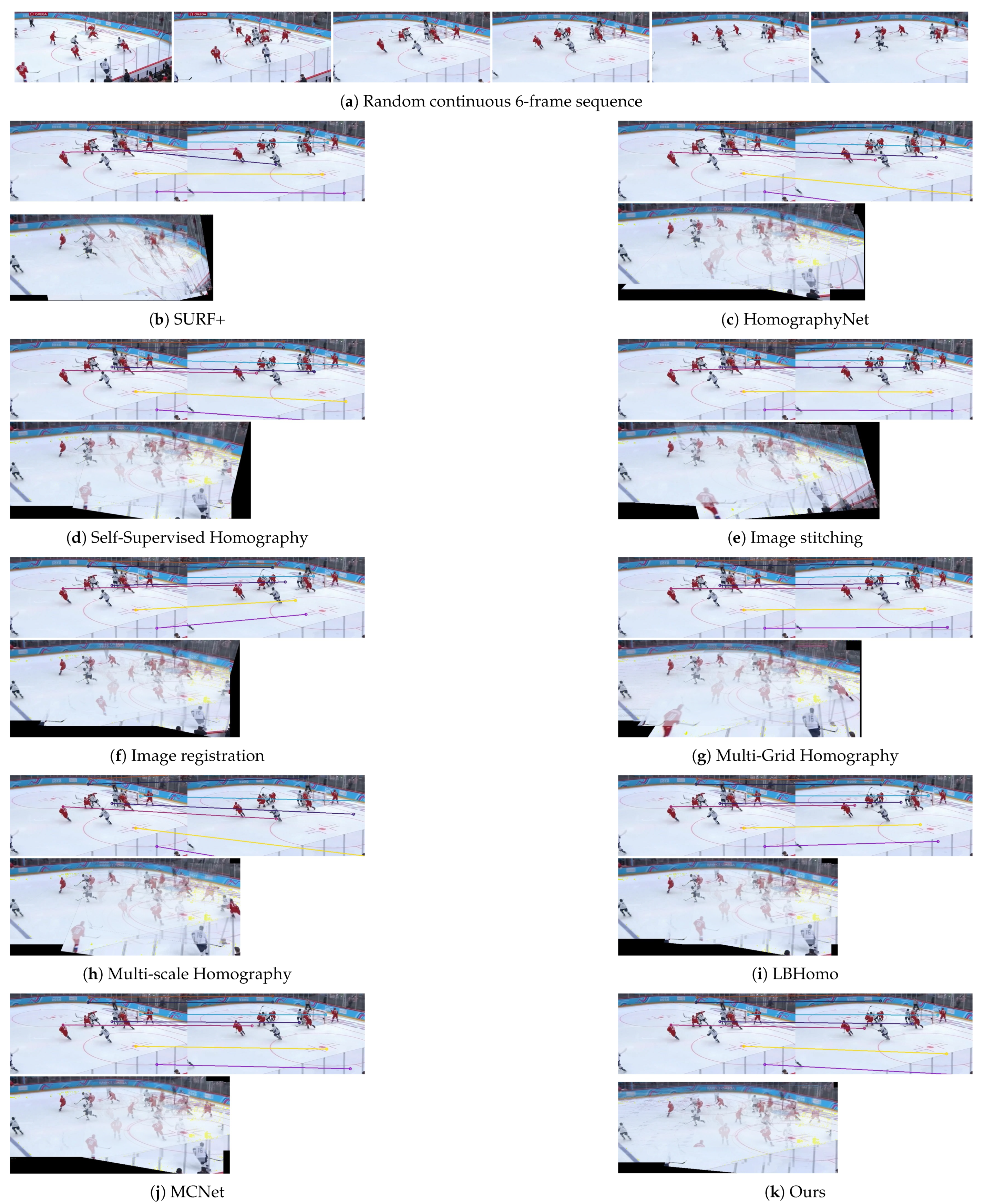
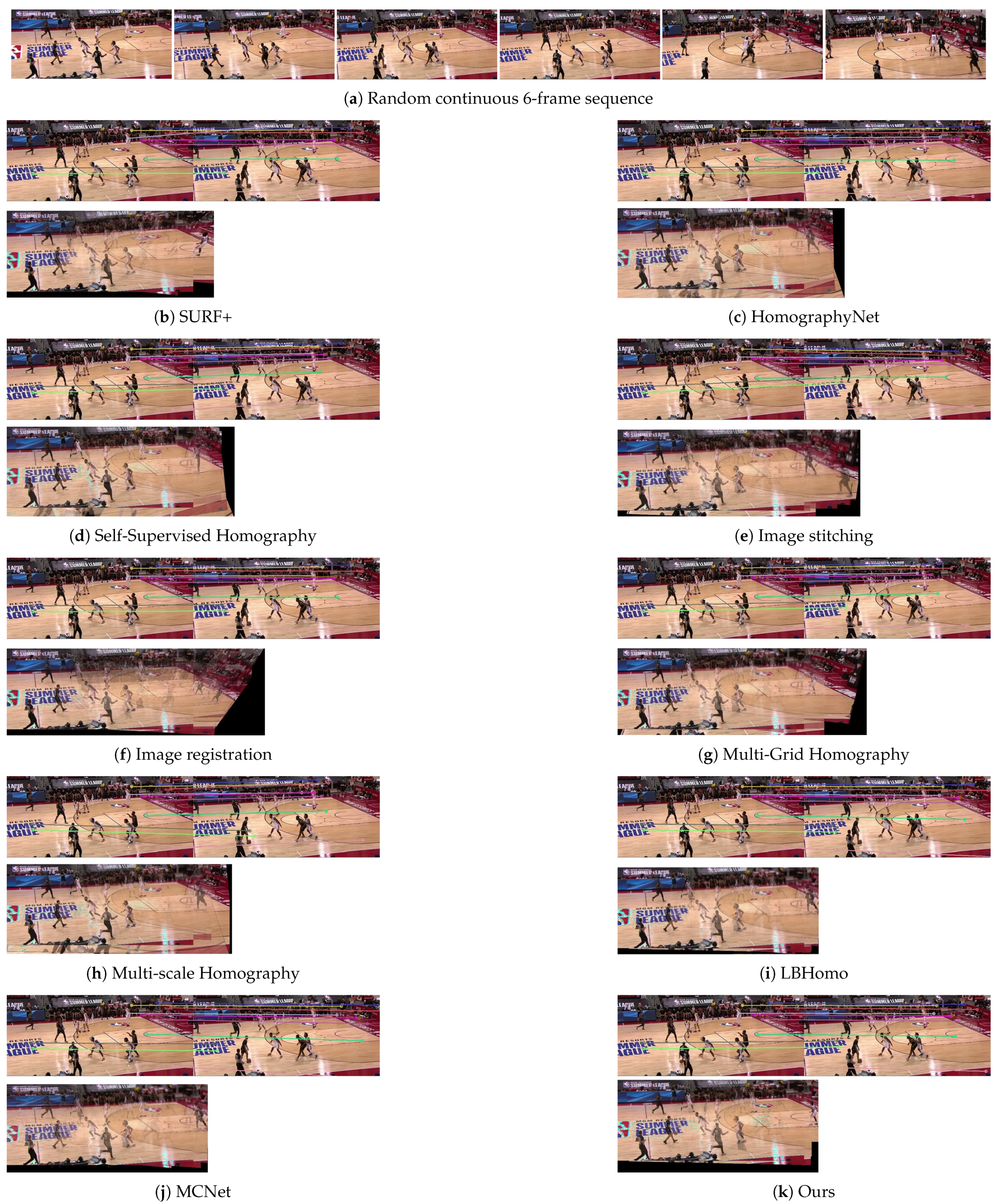
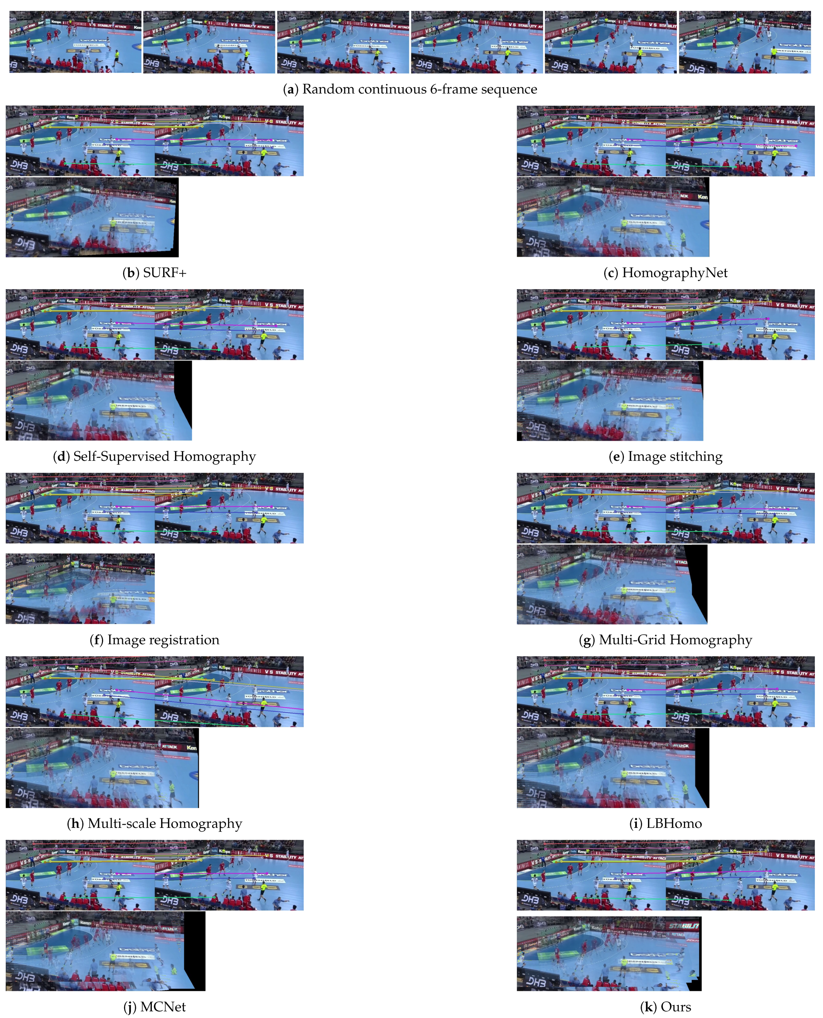
5.3. Comparison with State-of-the-Art Methods

In the experiment, comparison algorithms included the SURF+ keypoints-based method [47], the HomographyNet model [18], the deep learning model based on registration coordinate matrices [44,45], the image stitching algorithm via deep homography estimation [3], the Self-Supervised Deep Homography model [38], the Multi-Grid Deep Homography model [48], the Multi-Scale Homography model [49], the LBHomo model [40] and the MCNet model [50].

The visualization results, shown in Figure 10, Figure 11 and Figure 12, are derived from hockey, basketball, and handball competition videos. To provide a clearer representation of homography matrix predictions across consecutive multi-frame sequences, the resulting multi-frame images, obtained by applying homography transformations to adjacent paired images, are superimposed. The quantitative results are presented in

Table 4. All adjacent paired images.

Methods	Ice Hockey		Basketball		Handball
	${\mathit{H}}_{\mathit{acc}}(\%)$	${\mathit{B}}_{\mathit{acc}}(\%)$	${\mathit{H}}_{\mathit{acc}}(\%)$	${\mathit{B}}_{\mathit{acc}}(\%)$	${\mathit{H}}_{\mathit{acc}}(\%)$	${\mathit{B}}_{\mathit{acc}}(\%)$
SURF+ [47]	71.5	77.3	73.0	78.6	70.9	74.5
HomographyNet [18]	51.4	62.3	48.6	60.5	54.9	65.2
Self-Supervised Homography [38]	70.7	74.2	64.4	76.1	73.6	77.4
Image stitching [3]	74.0	78.5	74.7	81.1	76.5	82.6
Image registration [44,45]	72.6	77.8	73.2	80.4	71.8	79.7
Multi-Grid Homography [48]	74.3	79.6	71.6	79.5	74.3	81.8
Multi-scale Homography [49]	53.6	61.4	50.6	61.8	58.4	62.7
LBHomo [40]	75.2	79.1	75.1	80.2	77.5	82.3
MCNet [50]	71.3	74.9	70.5	78.7	73.2	79.4
Ours	76.4	80.4	77.6	81.8	80.7	83.5

and

Table 5. Initial and final frame paired images.

Methods	Ice Hockey		Basketball		Handball
	${\mathit{H}}_{\mathit{acc}}(\%)$	${\mathit{B}}_{\mathit{acc}}(\%)$	${\mathit{H}}_{\mathit{acc}}(\%)$	${\mathit{B}}_{\mathit{acc}}(\%)$	${\mathit{H}}_{\mathit{acc}}(\%)$	${\mathit{B}}_{\mathit{acc}}(\%)$
SURF+ [47]	65.5	73.8	68.9	77.1	66.4	78.4
HomographyNet [18]	54.0	67.5	59.7	67.1	56.8	66.2
Self-Supervised Homography [38]	63.4	73.5	60.5	68.3	69.1	71.4
Image stitching [3]	74.4	80.3	76.6	82.5	78.2	84.8
Image registration [44,45]	69.2	79.4	61.5	68.7	74.5	75.3
Multi-Grid Homography [48]	78.5	81.9	72.3	83.1	81.7	85.2
Multi-scale Homography [49]	57.8	64.5	60.2	65.7	50.1	62.3
LBHomo [40]	80.1	82.7	78.6	82.4	81.3	84.5
MCNet [50]	73.8	80.8	75.5	79.6	76.4	82.6
Ours	82.4	85.8	80.2	83.9	84.3	87.1

. Combined with the visualized experimental outcomes, it is evident that the proposed method outperforms others across the three ball game datasets. Existing homography transformation methods are primarily designed for single paired images with minimal content variation. As a result, they are generally better suited for predicting the homography matrix between adjacent paired images with small content changes.

Specifically, SURF+ [47] uses neighborhood gradient magnitude to compute its dominant orientation. By relying on the dominant orientation, it constructs keypoint-based local feature descriptions to achieve multimodal registration. While it is unaffected by data volume, the presence of numerous similar-colored regions on courts poses challenges for detecting and matching keypoints, particularly between the initial and final frames of sequence with significant content changes. Although HomographyNet [18] is an unsupervised network capable of automatically generating paired images with identical content for training, it still relies heavily on a substantial number of annotated paired images to improve prediction accuracy when content variations are present.

Self-Supervised Homography [38], similar to HomographyNet, utilizes a spatial transformation structure and optical flow loss in a self-supervised learning framework. While it is unaffected by data volume and well-suited for homography predictions between adjacent frames with minimal content changes, its ability to process competitive sports images with significant content variations remains limited.

The key components of the Image Stitching algorithm [3] are feature maps with progressively increased resolution, which are constructed in a hybrid manner. Its performance is influenced by data labeling, especially when the sequence is filmed in the same direction, as adjacent paired images often exhibit small parallax, enhancing the overall image stitching effect. Since our data labels describe the mapping relationship between the initial and final frames, the method relatively excels in evaluating homography prediction performance between these frames.

Image registration algorithms [44,45] utilize large-scale feature maps in the output layer to achieve pixel-wise image registration, requiring a substantial amount of paired keypoint annotation data. When data are insufficient, they tend to extract effective data pairs from similar images. Consequently, their testing performance is better for all adjacent image pairs compared to the initial and final frames.

Multi-Grid Homography model [48] improves homography matching by dividing the entire image matching process into block-wise matching and then comprehensively predicting the homography matrix to reduce errors. Although it is also influenced by data volume, it combines multi-scale contextual correlation, enhancing model performance and yielding relatively good experimental results.

Multi-Scale Homography model [49] improves performance by utilizing transformer modules to enhance the aggregation process of multi-scale features in dual channels. However, in our experiment, obtaining homography data labels proved costly. After training with limited data, it still exhibited poor prediction performance for homography matrices within two types of paired images.

The LBHomo model [40] shares a similar idea with our proposed method by breaking down large azimuth angle changes into a series of smaller ones using a progressive strategy. This significantly improves homography estimation accuracy in scenarios involving substantial azimuth variation. However, the experiments in the paper also show that the model is highly sensitive to the number of inserted intermediate images: too few result in insufficient optimization, while too many can lead to performance degradation due to accumulated errors. Furthermore, in our experimental image sequences, the content variation between paired images remains considerable, which causes the model’s performance to be suboptimal compared to our algorithm.

The MCNet model [50] is an iterative deep homography estimation network based on multi-scale correlation search. Its core innovation lies in the proposed multiscale correlation searching algorithm, which iteratively refines the homography matrix from low to high resolution. However, in competitive sports scenarios, stadiums often contain a large number of self-similar regions, which can significantly interfere with this search-based approach. As a result, the performance improvement observed during testing is limited.

By utilizing the invertibility property and decomposability property, our model not only demonstrates superior performance in predicting homography matrices between all adjacent paired images but also exhibits a more pronounced advantage between the initial and final frames. As shown in Figure 13, Figure 14 and Figure 15, further analysis reveals that our model outperforms competing methods. In testing across three types of competitive sports videos, the relatively suboptimal algorithm achieved a maximum relative improvement of 4.1% in $H_{acc}$ and 3.7% in $B_{acc}$. The average relative improvement across all compared algorithms was 20.3% in $H_{acc}$ and 13.5% in $B_{acc}$.

Overall, our symmetric model demonstrates more substantial gains in $H_{acc}$, although challenges persist in improving $B_{acc}$. This may be attributed to the fact that small variations in feature point positions can introduce significant errors in homography matrix calculations, indicating that enhancing $B_{acc}$, which predicts homography based on block regions, may provide more practical benefits. From a broader perspective, insufficient data introduces errors across all methods. While expanding the dataset is the most direct solution, it may significantly increase the data annotation workload.

6. Conclusions

This paper presents a symmetric network model and training approach for predicting continuous homography matrices between courts in a co-directional frame sequence, even with limited data annotation. The model leverages the mutual invertibility of bidirectional homography transformation matrices in paired images, enhancing accuracy in competitive sports videos with significant content changes. Furthermore, the model utilizes matrix decomposition to break down the homography matrix between the initial and final frames into multiple intermediate matrices corresponding to individual paired images within the frame sequence. By annotating only the homography matrix of the initial and final frames and applying an improved homography transformation calculation method, the neural network was effectively trained to achieve continuous prediction of homography matrices across co-directional frame sequences.

However, the experimental results reveal that even with our proposed method, a minimum error rate of 15% for all adjacent paired images and 10% for initial-to-final frame pairs persists. This suggests that CNNs may possess inherent limitations in effectively extracting features from competitive sports paired images, especially when substantial content variation occurs due to extended temporal intervals. To address this, future research will explore the removal of player regions from labeled sequence images using segmentation techniques and the development of a loss function that excludes these regions from calculation. This strategy aims to mitigate the interference caused by dynamic image content during CNN-based feature extraction. Furthermore, current methods are constrained to sequences captured from a single viewing direction—an idealized and limited scenario. Consequently, future work will focus on reducing the need for manual annotations, expanding the dataset diversity, and advancing techniques capable of predicting homography matrices across multi-directional frame sequences.

References

1. Agapito, L.; Hayman, E.; Reid, I. Self-Calibration of Rotating and Zooming Cameras. Int. J. Comput. Vis. 2001, 45, 107–127. [Google Scholar] [CrossRef]
2. Yu, J.; Da, F. Calibration refinement for a fringe projection profilometry system based on plane homography. Opt. Lasers Eng. 2021, 140, 106525. [Google Scholar] [CrossRef]
3. Zhao, Q.; Ma, Y.; Zhu, C.; Yao, C.; Feng, B.; Dai, F. Image stitching via deep homography estimation. Neurocomputing 2021, 450, 219–229. [Google Scholar] [CrossRef]
4. Nie, L.; Lin, C.; Liao, K.; Zhao, Y. Learning edge-preserved image stitching from multi-scale deep homography. Neurocomputing 2022, 491, 533–543. [Google Scholar] [CrossRef]
5. Finlayson, G.; Gong, H.; Fisher, R. Color Homography: Theory and Applications. IEEE Trans. Pattern Anal. Mach. Intell. 2019, 41, 20–33. [Google Scholar] [CrossRef]
6. Zhang, T.; Zhu, D.; Zhang, G.; Shi, W.; Liu, Y.; Zhang, X.; Li, J. Spatiotemporally Enhanced Photometric Loss for Self-Supervised Monocular Depth Estimation. In Proceedings of the 2022 IEEE/RSJ International Conference on Intelligent Robots and Systems (IROS), Kyoto, Japan, 23–27 October 2022; pp. 1–8. [Google Scholar] [CrossRef]
7. Mur-Artal, R.; Montiel, J.; Tardos, J. ORB-SLAM: A Versatile and Accurate Monocular SLAM System. IEEE Trans. Robot. 2015, 31, 1147–1163. [Google Scholar] [CrossRef]
8. Wang, H.; Chin, T.; Suter, D. Simultaneously Fitting and Segmenting Multiple-Structure Data with Outliers. IEEE Trans. Pattern Anal. Mach. Intell. 2012, 34, 1177–1192. [Google Scholar] [CrossRef]
9. Liu, S.; Chen, J.; Chang, C.; Ai, Y. A New Accurate and Fast Homography Computation Algorithm for Sports and Traffic Video Analysis. IEEE Trans. Circuits Syst. Video Technol. 2018, 28, 2993–3006. [Google Scholar] [CrossRef]
10. Liu, S.; Ye, N.; Wang, C.; Zhang, J.; Jia, L.; Luo, K.; Wang, J.; Sun, J. Content-Aware Unsupervised Deep Homography Estimation and its Extensions. IEEE Trans. Pattern Anal. Mach. Intell. 2023, 45, 2849–2863. [Google Scholar] [CrossRef]
11. Murino, V.; Castellani, U.; Etrari, A.; Fusiello, A. Registration of very time-distant aerial images. In Proceedings of the International Conference on Image Processing (ICIP), Rochester, NY, USA, 22–25 September 2002; pp. 989–992. [Google Scholar] [CrossRef]
12. Kaminski, J.; Shashua, A. Multiple View Geometry of General Algebraic Curves. Int. J. Comput. Vis. 2004, 56, 195–219. [Google Scholar] [CrossRef]
13. Hart, P. How the Hough transform was invented [DSP History]. IEEE Signal Process. Mag. 2009, 26, 18–22. [Google Scholar] [CrossRef]
14. Hu, M.; Chang, M.; Wu, J.; Chi, L. Robust Camera Calibration and Player Tracking in Broadcast Basketball Video. IEEE Trans. Multimed. 2011, 13, 266–279. [Google Scholar] [CrossRef]
15. Battikh, T.; Jabri, I. Camera calibration using court models for real-time augmenting soccer scenes. Multimed. Tools Appl. 2011, 51, 997–1011. [Google Scholar] [CrossRef]
16. Kim, H.; Sang, H. Robust image mosaicing of soccer videos using self-calibration and line tracking. Pattern Anal. Appl. 2001, 4, 9–19. [Google Scholar] [CrossRef]
17. Huang, C.; Pan, X.; Cheng, J.; Song, J. Deep Image Registration With Depth-Aware Homography Estimation. IEEE Signal Process. Lett. 2023, 30, 6–10. [Google Scholar] [CrossRef]
18. DeTone, D.; Malisiewicz, T.; Rabinovich, A. Deep image homography estimation. arXiv 2016, arXiv:1606.03798. [Google Scholar] [CrossRef]
19. Schuster, M.; Paliwal, K. Bidirectional recurrent neural networks. IEEE Trans. Signal Process. 1997, 45, 2673–2681. [Google Scholar] [CrossRef]
20. Derpanis, K. The Harris Corner Detector; York University: Toronto, ON, Canada, 2004; Volume 2, pp. 1–2. [Google Scholar]
21. Lowe, D. Distinctive image features from scale-invariant keypoints. Int. J. Comput. Vis. 2004, 60, 91–110. [Google Scholar] [CrossRef]
22. Yan, K.; Sukthankar, R. PCA-SIFT: A more distinctive representation for local image descriptors. In Proceedings of the 2004 IEEE Computer Society Conference on Computer Vision and Pattern Recognition (CVPR), Washington, DC, USA, 27 June–2 July 2004; p. 2. [Google Scholar] [CrossRef]
23. Ojala, T.; Pietikainen, M.; Maenpaa, T. Multiresolution gray-scale and rotation invariant texture classification with local binary patterns. IEEE Trans. Pattern Anal. Mach. Intell. 2002, 24, 971–987. [Google Scholar] [CrossRef]
24. Bay, H.; Tuytelaars, T.; Van, G.L. Surf: Speeded up robust features. Lecture notes in computer science. In Proceeding of the 9th European Conference on Computer Vision (ECCV), Graz, Austria, 7–13 May 2006; pp. 404–417. [Google Scholar] [CrossRef]
25. Yao, Q.; Kubota, A.; Kawakita, K.; Nonaka, K.; Sankoh, H.; Naito, S. Fast camera self-calibration for synthesizing Free Viewpoint soccer Video. In Proceedings of the 2017 IEEE International Conference on Acoustics, Speech and Signal Processing (ICASSP), New Orleans, LA, USA, 2–9 March 2017; pp. 1612–1616. [Google Scholar] [CrossRef]
26. Zeng, R.; Lakemond, R.; Denman, S.; Sridharan, S.; Fookes, C.; Morgan, S. Calibrating Cameras in Poor-Conditioned Pitch-Based Sports Games. In Proceedings of the 2018 IEEE International Conference on Acoustics, Speech and Signal Processing (ICASSP), Calgary, AB, Canada, 6–11 June 2018; pp. 1902–1906. [Google Scholar] [CrossRef]
27. Bozorgpour, A.; Fotouhi, M.; Kasaei, S. Robust homography optimization in soccer scenes. In Proceedings of the 2015 23rd Iranian Conference on Electrical Engineering, Tehran, Iran, 10–14 May 2015; pp. 787–792. [Google Scholar] [CrossRef]
28. Lao, Y.; Ait-Aider, O. Rolling Shutter Homography and its Applications. IEEE Trans. Pattern Anal. Mach. Intell. 2021, 43, 2780–2793. [Google Scholar] [CrossRef]
29. Wang, X.; Wang, C.; Bai, X.; Liu, Y.; Zhou, J. Deep homography estimation with pairwise invertibility constraint. In Proceedings of the Structural, Syntactic, and Statistical Pattern Recognition: Joint IAPR International Workshop, Beijing, China, 17–19 August 2018; pp. 204–214. [Google Scholar] [CrossRef]
30. Czolbe, S.; Krause, O.; Feragen, A. DeepSim: Semantic similarity metrics for learned image registration. arXiv 2020, arXiv:2011.05735. [Google Scholar] [CrossRef]
31. Ghassab, V.; Maanicshah, K.; Bouguila, N.; Green, P. REP-Model: A deep learning framework for replacing ad billboards in soccer videos. In Proceedings of the 2020 IEEE International Symposium on Multimedia (ISM), Naples, Italy, 29 November–1 December 2020; pp. 149–153. [Google Scholar] [CrossRef]
32. Molina-Cabello, M.; Garcia-Gonzalez, J.; Luque-Baena, R.; Thurnhofer-Hemsi, K.; Lopez-Rubio, E. Adaptive estimation of optimal color transformations for deep convolutional network based homography estimation. In Proceedings of the 2020 25th International Conference on Pattern Recognition (ICPR), Milan, Italy, 10–15 January 2021; pp. 3106–3113. [Google Scholar] [CrossRef]
33. Zeng, L.; Du, Y.; Lin, H.; Wang, J.; Yin, J.; Yang, J. A Novel Region-Based Image Registration Method for Multisource Remote Sensing Images Via CNN. IEEE J. Sel. Top. Appl. Earth Observ. Remote Sens. 2021, 14, 1821–1831. [Google Scholar] [CrossRef]
34. Wang, G.; You, Z.; An, P.; Yu, J.; Chen, Y. Efficient and robust homography estimation using compressed convolutional neural network. In Proceedings of the Digital TV and Multimedia Communication: 15th International Forum, Shanghai, China, 20–21 September 2018; pp. 156–168. [Google Scholar] [CrossRef]
35. Ding, T.; Yang, Y.; Zhu, Z.; Robinson, D.; Vidal, R.; Kneip, L.; Tsakiris, M. Robust Homography Estimation via Dual Principal Component Pursuit. In Proceedings of the IEEE/CVF Conference on Computer Vision and Pattern Recognition (CVPR), Seattle, WA, USA, 13–19 June 2020; pp. 6079–6088. [Google Scholar] [CrossRef]
36. Li, B.; Zhang, J.; Yang, R.; Li, H. FM-Net: Deep Learning Network for the Fundamental Matrix Estimation from Biplanar Radiographs. Comput. Meth. Programs Biomed. 2022, 220, 106782. [Google Scholar] [CrossRef]
37. Nguyen, T.; Chen, S.W.; Shivakumar, S.S.; Taylor, C.J. Unsupervised deep homography: A fast and robust homography estimation model. IEEE Robot. Autom. Lett. 2018, 3, 2346–2353. [Google Scholar] [CrossRef]
38. Wang, C.; Wang, X.; Bai, X.; Liu, Y.; Zhou, J. Self-Supervised deep homography estimation with invertibility constraints. Pattern Recognit. Lett. 2019, 128, 355–360. [Google Scholar] [CrossRef]
39. Koguciuk, D.; Arani, E.; Zonooz, B. Perceptual loss for robust unsupervised homography estimation. In Proceedings of the IEEE/CVF conference on computer vision and pattern recognition, Online, 19–25 June 2021; pp. 4274–4283. [Google Scholar] [CrossRef]
40. Jiang, H.; Li, H.; Lu, Y.; Han, S.; Liu, S. Semi-supervised deep large-baseline homography estimation with progressive equivalence constraint. In Proceedings of the AAAI Conference on Artificial Intelligence, Washington, DC, USA, 7–14 February 2023; pp. 1024–1032. [Google Scholar] [CrossRef]
41. Youku. Available online: https://v.youku.com/video?spm=a2hkm.8166622.PhoneSokuUgc_1.dscreenshot&&vid=XNTEzNjY3NzU4MA==&playMode=pugv&frommaciku=1 (accessed on 21 May 2025).
42. Tencent Video. Available online: https://v.qq.com/x/cover/mzc00200q077ncj/m0046rerfdq.html (accessed on 21 May 2025).
43. Youku. Available online: https://v.youku.com/video?spm=a2hkm.8166622.PhoneSokuUgc_1.dscreenshot&&vid=XNDA1NDc1NDA1Mg==&playMode=pugv&frommaciku=1 (accessed on 21 May 2025).
44. Huang, C.W.; Cheng, J.C.; Pan, X. Pixel-wise visible image registration based on deep neural network. J. Beijing Univ. Aeronaut. Astronaut. 2022, 48, 522–532. [Google Scholar] [CrossRef]
45. Jiang, Q.; Liu, Y.; Fang, J.; Yan, Y.; Jiang, X. Registration method for power equipment infrared and visible images based on contour feature. Chin. J. Sci. Instrum. 2022, 41, 252–260. [Google Scholar] [CrossRef]
46. Cao, X.; Yang, J.; Zhang, J.; Wang, Q.; Yap, P.; Shen, D. Deformable Image Registration Using a Cue-Aware Deep Regression Network. IEEE Trans. Biomed. Eng. 2018, 65, 1900–1911. [Google Scholar] [CrossRef] [PubMed]
47. Zhao, D.; Yang, Y.; Ji, Z.; Hu, X. Rapid multimodality registration based on MM-SURF. Neurocomputing 2014, 131, 87–97. [Google Scholar] [CrossRef]
48. Nie, L.; Lin, C.; Liao, K.; Liu, S.; Zhao, Y. Depth-Aware Multi-Grid Deep Homography Estimation With Contextual Correlation. IEEE Trans. Circuits Syst. Video Technol. 2022, 32, 4460–4472. [Google Scholar] [CrossRef]
49. Li, Y.; Chen, K.; Sun, S.; He, C. Multi-scale homography estimation based on dual feature aggregation transformer. IET Image Process. 2023, 17, 1403–1416. [Google Scholar] [CrossRef]
50. Zhu, H.; Cao, S.Y.; Hu, J.; Zuo, S.; Yu, B.; Ying, J. MCNet: Rethinking the core ingredients for accurate and efficient homography estimation. In Proceedings of the IEEE/CVF Conference on Computer Vision and Pattern Recognition, Seattle, WA, USA, 17–21 June 2024; pp. 25932–25941. [Google Scholar]
Figure 1. Schematic diagram of direct and indirect predictions of the homography matrix in team ball sports competitions.
Symmetry 17 00832 g001
Figure 2. Overall architecture. After each round of training is completed, the parameters of the five H-Nets are averaged and shared. The ‘*’ represents matrix multiplication.
Symmetry 17 00832 g002
Figure 3. Schematic diagram of bidirectional homography transformation of stacked unit. H-Net represents the identical network architecture, and OUT indicates the positional deviation of 4 specific key points. The ‘*’ represents matrix multiplication.
Symmetry 17 00832 g003
Figure 4. Key point selection strategy.
Symmetry 17 00832 g004
Figure 5. The matching effect achieves through a random Homography transformation on the same court screen using the HomographyNet after pre-training. The source perspective is indicated by the blue box, while the target perspective is represented by the red box.
Symmetry 17 00832 g005
Figure 6. Experimental results of homography transformation in ice hockey competition. The source perspective is indicated by the blue box, while the target perspective is represented by the red box.
Symmetry 17 00832 g006
Figure 7. Experimental results of homography transformation in basketball competition. The source perspective is indicated by the blue box, while the target perspective is represented by the red box.
Symmetry 17 00832 g007
Figure 8. Experimental results of homography transformation in handball competition. The source perspective is indicated by the blue box, while the target perspective is represented by the red box.
Symmetry 17 00832 g008
Figure 9. The growth rate of the test results for initial and final frame paired images relative to the test results for all adjacent paired images.
Symmetry 17 00832 g009
Figure 10. The experimental results of the homography matrix between six frames from the ice hockey competition video. The left side of the subgraphs displays the random keypoint matching and mapping between the 3rd and 4th frames, while the right side shows the superposition of all images after applying a unified mapping transformation.
Symmetry 17 00832 g010
Figure 11. The experimental results of the homography matrix between six frames from the basketball competition video. The left side of subgraphs displays the random keypoint matching and mapping between the 3rd and 4th frames, while the right side shows the superposition of all images after applying a unified mapping transformation.
Symmetry 17 00832 g011
Figure 12. The experimental results of the homography matrix between six frames from the handball competition video. The left side of the subgraphs displays the random keypoint matching and mapping between the 3rd and 4th frames, while the right side shows the superposition of all images after applying a unified mapping transformation.
Symmetry 17 00832 g012
Figure 13. The Relative Growth Rate (RGR) for the Ice Hockey.
Symmetry 17 00832 g013
Figure 14. The Relative Growth Rate for the Basketball.
Symmetry 17 00832 g014
Figure 15. The Relative Growth Rate for the Handball.
Symmetry 17 00832 g015