

Statistical Inference of Inverse Weibull Distribution Under Joint Progressive Censoring Scheme


Abstract
1. Introduction
2. The Joint Progressive Type II Censor Scheme and Maximum Likelihood Estimation
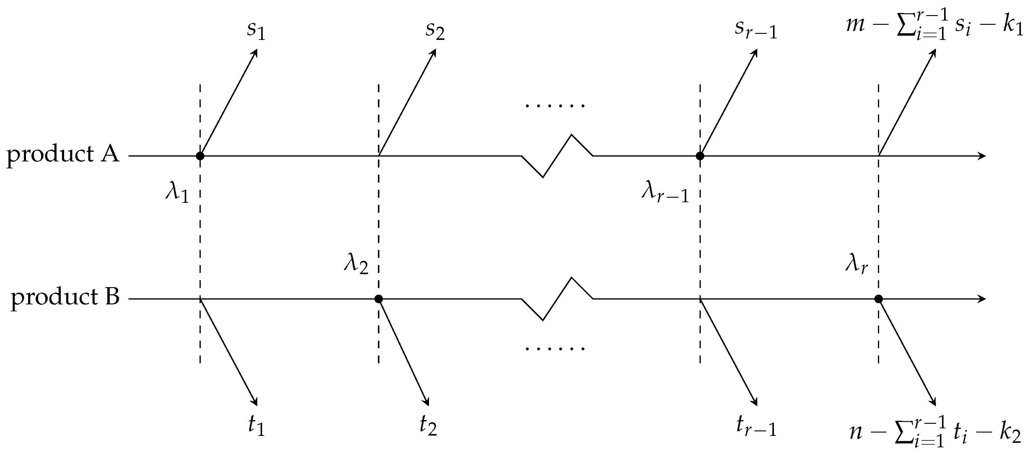
2.1. Model Description
2.2. Maximum Likelihood Estimation
3. Approximate Confidence Interval
4. Bootstrap Confidence Intervals
| Algorithm 1 Generation process of Boot-P CIs |
|
| Algorithm 2 Generation process of Boot-T CIs |
|
5. Bayesian Inference
5.1. Prior and Posterior Distribution
5.2. Loss Functions
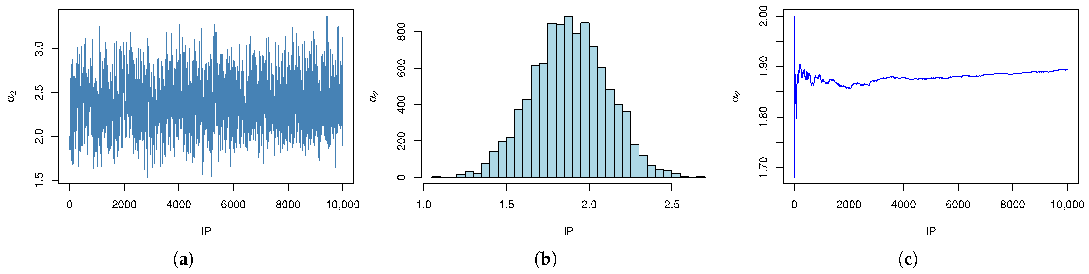
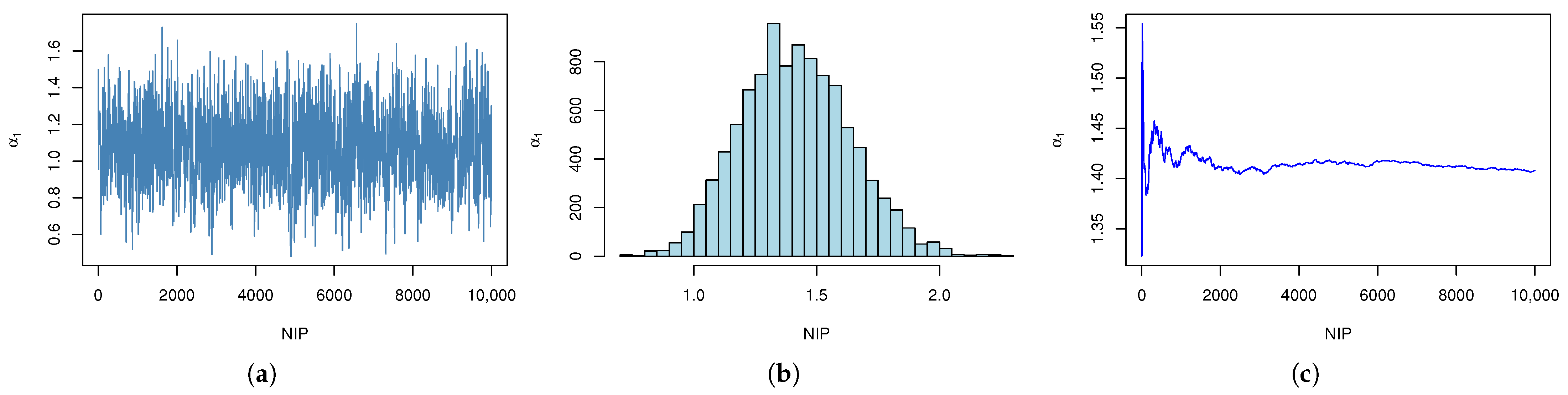
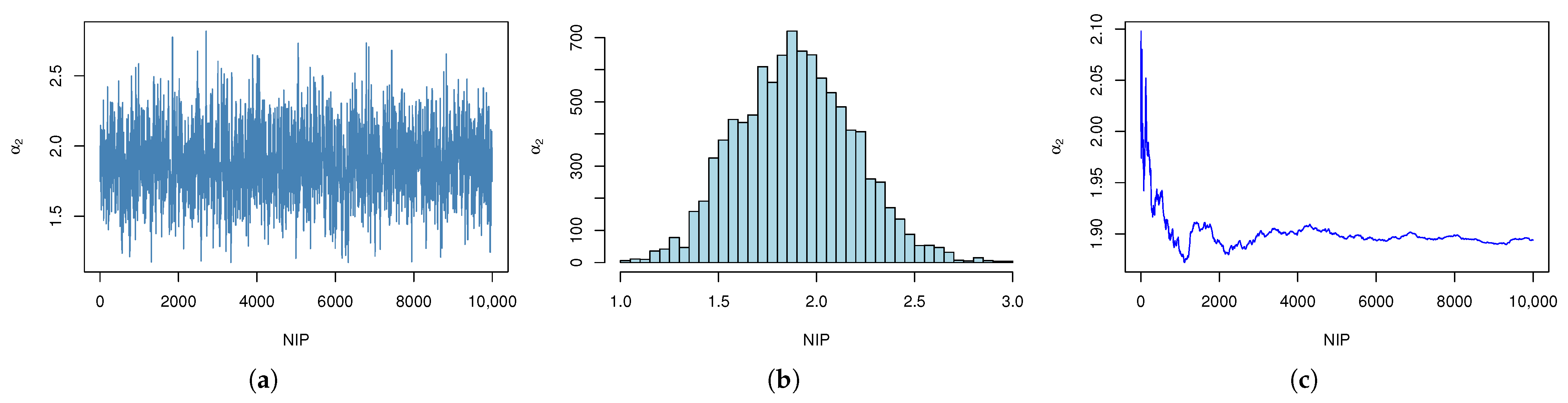
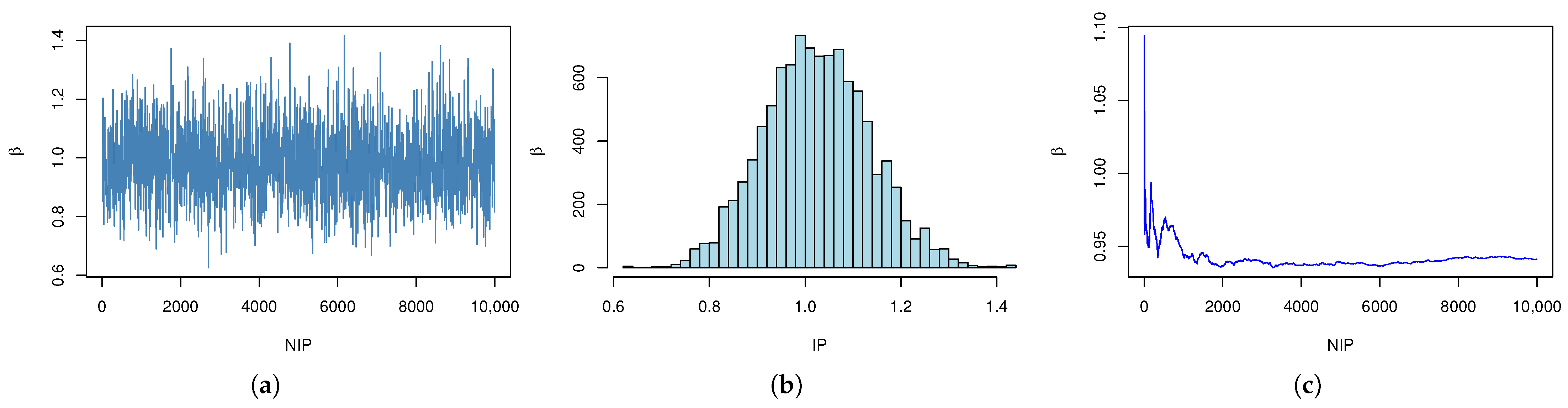
5.3. Metropolis–Hastings Algorithm
| Algorithm 3 Generating samples following the posterior distribution. |
|
6. Simulation Study
| Algorithm 4 The algorithm to generate samples under the JPC scheme. |
|
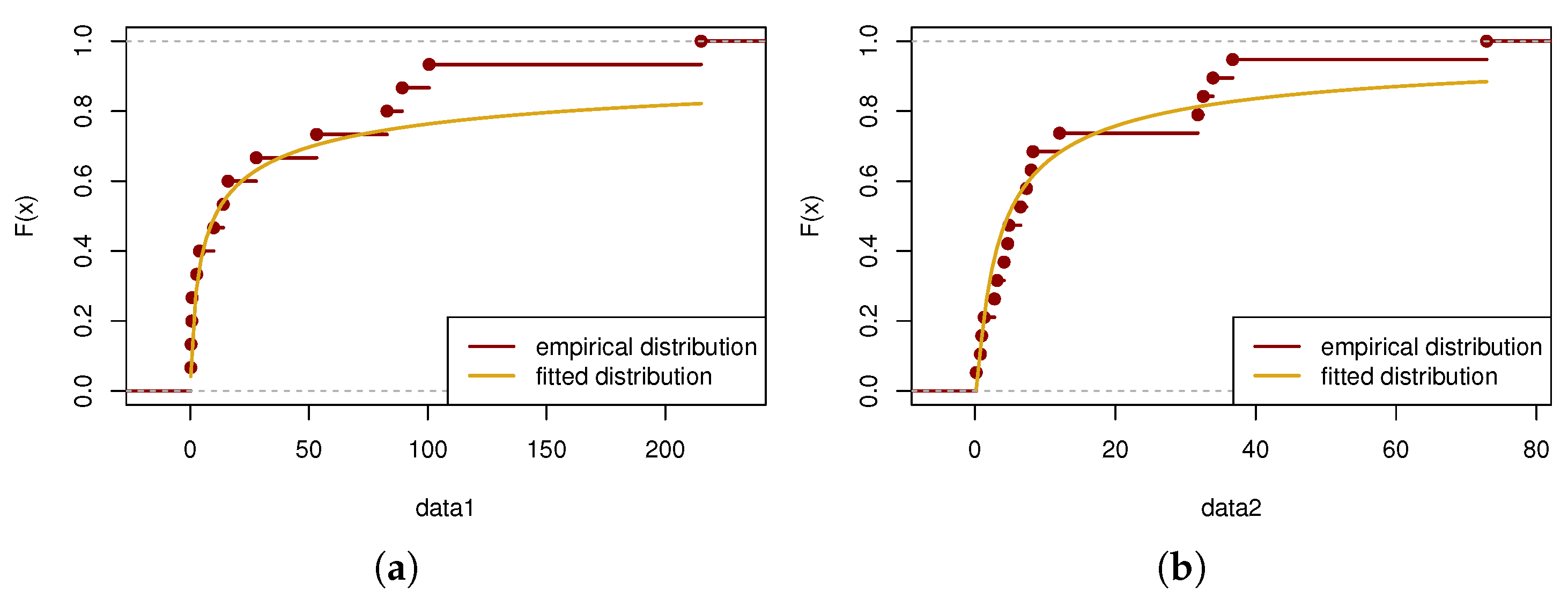
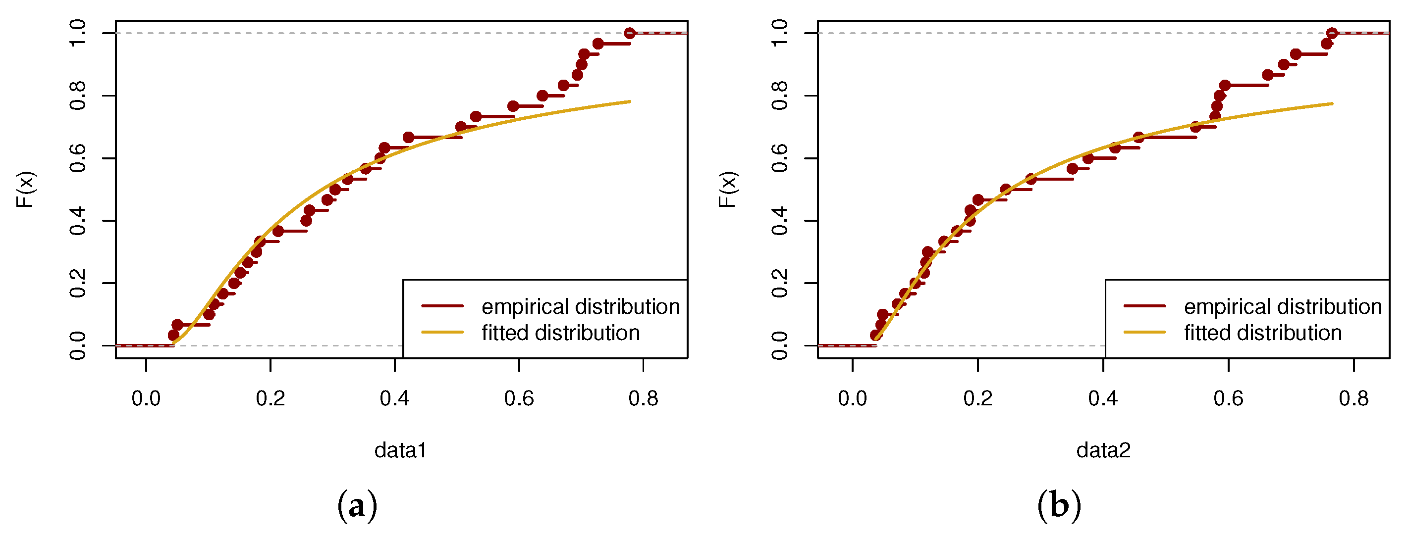
7. Real-Data Analysis
7.1. Example 1
7.2. Example 2
8. Conclusions
Author Contributions
Funding
Data Availability Statement
Conflicts of Interest
Appendix A

| r | SE | LINEX (a = −2) | LINEX (a = 2) | |||||
|---|---|---|---|---|---|---|---|---|
| ABE (MSE) | AL (CP) | ABE (MSE) | AL (CP) | ABE (MSE) | AL (CP) | |||
| (20, 20) | 20 | (, 20) | 2.0450 | 1.0578 | 2.0809 | 1.0693 | 1.9500 | 1.0111 |
| (0.4506) | (89.8%) | (0.4816) | (79.6%) | (0.4609) | (81.5%) | |||
| (, 5, 15) | 2.1021 | 1.0609 | 2.1178 | 1.0927 | 2.1783 | 1.0453 | ||
| (0.4411) | (87.8%) | (0.4668) | (81.6%) | (0.4431) | (83.7%) | |||
| 30 | (, 10) | 1.9845 | 1.0349 | 2.0268 | 1.0534 | 2.0539 | 1.0484 | |
| (0.4671) | (83.7%) | (0.4497) | (81.6%) | (0.4357) | (91.8%) | |||
| (, 8, 2) | 2.0108 | 1.0205 | 2.0720 | 1.0617 | 2.0798 | 1.0027 | ||
| (0.4473) | (81.6%) | (0.4538) | (79.6%) | (0.4315) | (83.6%) | |||
| (20, 30) | 30 | (, 20) | 1.9817 | 0.9924 | 1.9778 | 0.9908 | 2.0006 | 1.0493 |
| (0.4466) | (87.6%) | (0.4440) | (82.6%) | (0.4557) | (81.6%) | |||
| (, 15, 5) | 2.0685 | 1.0816 | 2.0401 | 1.1127 | 2.1827 | 1.0594 | ||
| (0.4478) | (87.8%) | (0.4863) | (79.6%) | (0.4652) | (79.9%) | |||
| 40 | (, 10) | 2.04347 | 1.0405 | 2.0923 | 0.9916 | 1.9950 | 1.0081 | |
| (0.4413) | (83.7%) | (0.4240) | (79.6%) | (0.4425) | (81.6%) | |||
| (, 5, 5) | 2.1766 | 1.0795 | 2.1314 | 1.0499 | 2.1675 | 1.0308 | ||
| (0.4463) | (89.8%) | (0.4631) | (83.7%) | (0.4570) | (83.7%) | |||
| (30, 30) | 30 | (, 30) | 2.0053 | 0.9472 | 1.9902 | 1.0067 | 1.9895 | 0.9612 |
| (0.4272) | (75.51%) | (0.4457) | (77.55%) | (0.4396) | (75.51%) | |||
| (, 20, 10) | 2.0856 | 1.0137 | 2.0936 | 1.0367 | 2.1222 | 1.0803 | ||
| (0.4360) | (86.6%) | (0.4442) | (81.6%) | (0.4659) | (81.6%) | |||
| 40 | (, 20) | 1.9899 | 0.9520 | 2.0082 | 0.9922 | 2.0309 | 1.0350 | |
| (0.4474) | (79.4%) | (0.4364) | (83.3%) | (0.4418) | (79.6%) | |||
| (, 20, 0) | 2.0348 | 1.0415 | 1.9278 | 1.0335 | 2.0416 | 1.0677 | ||
| (0.4396) | (75.5%) | (0.4337) | (79.6%) | (0.4442) | (87.8%) | |||
| (30, 40) | 40 | (, 30) | 1.9494 | 1.0339 | 2.0150 | 1.0022 | 1.9939 | 1.0178 |
| (0.4650) | (83.7%) | (0.4368) | (85.7%) | (0.4475) | (79.5%) | |||
| (, 29, 1) | 2.0865 | 1.0234 | 2.0493 | 1.0191 | 1.9992 | 1.0813 | ||
| (0.4341) | (77.5%) | (0.4269) | (83.7%) | (0.4478) | (85.5%) | |||
| 50 | (, 20) | 1.9888 | 1.0524 | 2.0223 | 0.9736 | 1.9990 | 1.0195 | |
| (0.4689) | (77.6%) | (0.4222) | (81.4%) | (0.4347) | (83.7%) | |||
| (, 15, 5) | 2.0936 | 1.0050 | 2.0224 | 1.0218 | 2.0535 | 0.9626 | ||
| (0.4542) | (83.5%) | (0.4452) | (83.7%) | (0.4511) | (87.3%) | |||
| (40, 50) | 50 | (, 40) | 1.9598 | 1.0426 | 2.0210 | 1.0241 | 2.0131 | 1.0456 |
| (0.4476) | (81.6%) | (0.4403) | (82.6%) | (0.4434) | (83.7%) | |||
| (, 35, 5) | 2.0447 | 1.0120 | 2.0411 | 1.0143 | 2.1582 | 1.0381 | ||
| (0.4362) | (89.6%) | (0.4293) | (87.6%) | (0.4232) | (85.7%) | |||
| 60 | (, 30) | 1.9892 | 0.9726 | 2.0064 | 0.9821 | 2.0210 | 1.0211 | |
| (0.4316) | (82.3%) | (0.4224) | (81.6%) | (0.4438) | (81.6%) | |||
| (, 25, 5) | 2.1037 | 1.0502 | 2.1364 | 1.1039 | 2.0656 | 1.0532 | ||
| (0.4493) | (79.5%) | (0.4643) | (85.7%) | (0.4398) | (85.7%) | |||
| r | SE | LINEX (a = −2) | LINEX (a = 2) | |||||
|---|---|---|---|---|---|---|---|---|
| ABE (MSE) | AL (CP) | ABE (MSE) | AL (CP) | ABE (MSE) | AL (CP) | |||
| (20, 20) | 20 | (, 20) | 0.9937 | 1.0954 | 1.0039 | 1.0611 | 1.0180 | 1.0334 |
| (0.5189) | (83.7%) | (0.4993) | (79.4%) | (0.4800) | (76.4%) | |||
| (, 5, 15) | 0.9781 | 1.0944 | 0.9458 | 1.0991 | 1.0212 | 1.1931 | ||
| (0.4930) | (83.7%) | (0.5209) | (77.6%) | (0.6462) | (79.3%) | |||
| 30 | (, 10) | 0.9949 | 1.0573 | 1.0050 | 0.9868 | 0.9992 | 1.0741 | |
| (0.4900) | (77.6%) | (0.4175) | (77.3%) | (0.4891) | (75.5%) | |||
| (, 8, 2) | 1.0452 | 0.9798 | 0.9985 | 1.0683 | 0.9623 | 1.0461 | ||
| (0.4417) | (79.5%) | (0.5132) | (81.4%) | (0.4756) | (83.7%) | |||
| (20, 30) | 30 | (, 20) | 1.0068 | 1.0603 | 1.0278 | 1.0255 | 1.0388 | 0.9640 |
| (0.4847) | (75.5%) | (0.4776) | (85.3%) | (0.4477) | (79.2%) | |||
| (, 15, 5) | 0.9781 | 1.0944 | 0.9458 | 1.0991 | 1.0212 | 1.1931 | ||
| (0.4930) | (83.7%) | (0.5209) | (77.6%) | (0.6462) | (79.3%) | |||
| 40 | (, 10) | 0.9963 | 1.0729 | 1.0238 | 1.0067 | 1.0040 | 0.9967 | |
| (0.5050) | (79.4%) | (0.4489) | (79.4%) | (0.4339) | (85.7%) | |||
| (, 5, 5) | 0.9807 | 1.1703 | 1.0075 | 1.0950 | 1.0316 | 1.0621 | ||
| (0.5575) | (79.5%) | (0.4910) | (81.6%) | (0.4717) | (83.5%) | |||
| (30, 30) | 30 | (, 30) | 1.0107 | 1.0005 | 1.0055 | 1.0291 | 0.9876 | 1.0327 |
| (0.4328) | (81.6%) | (0.4670) | (77.3%) | (0.4569) | (79.6%) | |||
| (, 20, 10) | 0.9806 | 1.0525 | 1.0169 | 1.0173 | 1.0068 | 1.0439 | ||
| (0.5004) | (79.2%) | (0.4542) | (83.5%) | (0.5093) | (82.4%) | |||
| 40 | (, 20) | 0.9948 | 0.9146 | 1.0206 | 0.9266 | 1.0067 | 1.0614 | |
| (0.3782) | (85.5%) | (0.4180) | (81.2%) | (0.4759) | (83.5%) | |||
| (, 20, 0) | 1.0030 | 1.0366 | 1.0168 | 1.0279 | 1.0014 | 1.0452 | ||
| (0.4935) | (80.1%) | (0.4827) | (85.2%) | (0.4877) | (83.4%) | |||
| (30, 40) | 40 | (, 30) | 0.985 | 1.098 | 1.026 | 0.990 | 1.019 | 1.019 |
| (0.5126) | (79.6%) | (0.4305) | (71.4%) | (0.4581) | (69.4%) | |||
| (, 29, 1) | 1.0223 | 1.0315 | 1.0313 | 0.9991 | 1.0161 | 1.0187 | ||
| (0.4671) | (77.3%) | (0.4496) | (81.2%) | (0.4723) | (75.3%) | |||
| 50 | (, 20) | 0.9933 | 0.9981 | 0.9999 | 1.0085 | 1.0143 | 0.9847 | |
| (0.4293) | (82.6%) | (0.4293) | (83.6%) | (0.4359) | (80.2%) | |||
| (, 15, 5) | 0.9964 | 1.0625 | 1.0076 | 1.0580 | 0.9790 | 1.0990 | ||
| (0.4780) | (71.4%) | (0.4708) | (79.6%) | (0.4960) | (73.5%) | |||
| (40, 50) | 50 | (, 40) | 0.9993 | 0.9993 | 1.0055 | 1.0000 | 0.9928 | 1.0416 |
| (0.4184) | (79.5%) | (0.4306) | (77.6%) | (0.4404) | (85.7%) | |||
| (, 35, 5) | 0.9947 | 1.0350 | 0.9744 | 1.0048 | 0.9747 | 1.1015 | ||
| (0.4617) | (79.6%) | (0.4355) | 86.4%) | (0.5212) | (78.4%) | |||
| 60 | (, 30) | 1.0000 | 1.0013 | 1.0016 | 0.9956 | 1.0090 | 1.0714 | |
| (0.4469) | (85.3%) | (0.4297) | (79.5%) | (0.4790) | (83.5%) | |||
| (, 25, 5) | 0.9860 | 1.0654 | 0.9819 | 1.1362 | 1.0007 | 1.0541 | ||
| (0.4726) | (79.6%) | (0.5216) | (81.6%) | (0.4794) | (83.7%) | |||
| r | SE | LINEX (a = −2) | LINEX (a = 2) | |||||
|---|---|---|---|---|---|---|---|---|
| ABE (MSE) | AL (CP) | ABE (MSE) | AL (CP) | ABE (MSE) | AL (CP) | |||
| (20, 20) | 20 | (, 20) | 2.1369 | 1.1184 | 2.1172 | 1.0649 | 2.1362 | 1.0704 |
| (0.5073) | (83.7%) | (0.5054) | (78.6%) | (0.5017) | (83.5%) | |||
| (, 5, 15) | 2.2611 | 1.2195 | 2.2837 | 1.0999 | 2.2413 | 1.2725 | ||
| (0.5829) | (87.8%) | (0.5677) | (85.7%) | (0.5045) | (95.9%) | |||
| 30 | (, 10) | 2.1079 | 1.1118 | 2.0560 | 1.0222 | 1.9763 | 1.0789 | |
| (0.4709) | (87.8%) | (0.4957) | (83.5%) | (0.4851) | (85.5%) | |||
| (, 8, 2) | 2.1212 | 1.1070 | 2.2686 | 1.0659 | 2.1452 | 1.0980 | ||
| (0.4977) | (77.6%) | (0.4464) | (83.7%) | (0.4805) | (83.7%) | |||
| (20, 30) | 30 | (, 20) | 1.9937 | 1.0379 | 2.0300 | 0.9538 | 2.1100 | 1.0113 |
| (0.4733) | (83.5%) | (0.4905) | (80.1%) | (0.4708) | (79.6%) | |||
| (, 15, 5) | 2.1332 | 1.1378 | 2.2554 | 1.0695 | 2.2903 | 1.1828 | ||
| (0.4858) | (89.8%) | (0.4885) | (83.7%) | (0.5124) | (83.7%) | |||
| 40 | (, 10) | 1.9805 | 1.0449 | 1.9661 | 1.0533 | 2.0159 | 1.0594 | |
| (0.4789) | (81.4%) | (0.4404) | (83.7%) | (0.4919) | (75.5%) | |||
| (, 5, 5) | 2.1549 | 1.0898 | 2.2024 | 1.1304 | 2.2637 | 1.1337 | ||
| (0.4618) | (83.7%) | (0.5000) | (83.7%) | (0.5218) | (81.6%) | |||
| (30, 30) | 30 | (, 30) | 2.0202 | 1.1449 | 2.0038 | 1.0791 | 2.0269 | 1.0245 |
| (0.5005) | (83.7%) | (0.4847) | (77.6%) | (0.4466) | (81.6%) | |||
| (, 20, 10) | 2.2779 | 1.0953 | 2.1466 | 1.0463 | 2.1271 | 1.0983 | ||
| (0.4688) | (79.6%) | (0.4722) | (80.3%) | (0.4939) | (79.6%) | |||
| 40 | (, 20) | 2.0315 | 1.0394 | 2.0478 | 1.0209 | 1.9222 | 1.0062 | |
| (0.4481) | (83.7%) | (0.4735) | (79.4%) | (0.4616) | (85.6%) | |||
| (, 20, 0) | 2.0522 | 1.0282 | 2.0611 | 1.0041 | 2.0038 | 1.0683 | ||
| (0.4450) | (86.6%) | (0.4517) | (79.6%) | (0.4733) | (79.6%) | |||
| (30, 40) | 40 | (, 30) | 2.1336 | 1.0689 | 2.0433 | 1.0620 | 2.0762 | 1.0605 |
| (0.4662) | (77.6%) | (0.4636) | (81.6%) | (0.4551) | (85.7%) | |||
| (, 29, 1) | 2.0341 | 0.9790 | 2.1279 | 1.0885 | 2.0263 | 1.0263 | ||
| (0.4332) | (75.5%) | (0.4606) | (91.8%) | (0.4820) | (85.3%) | |||
| 50 | (, 20) | 2.0932 | 1.0310 | 1.9805 | 0.9660 | 2.0880 | 1.0606 | |
| (0.4436) | (79.6%) | (0.4270) | (63.3%) | (0.4548) | (75.5%) | |||
| (, 15, 5) | 2.1114 | 1.0367 | 2.0779 | 1.0468 | 2.1596 | 1.0724 | ||
| (0.4478) | (73.5%) | (0.4443) | (87.8%) | (0.4442) | (89.8%) | |||
| (40, 50) | 50 | (, 40) | 1.9494 | 0.9671 | 1.9803 | 0.9992 | 2.0339 | 1.0119 |
| (0.4416) | (81.4%) | (0.4323) | (77.5%) | (0.4348) | (81.6%) | |||
| (, 35, 5) | 2.0959 | 1.0594 | 2.0835 | 1.0281 | 2.2055 | 1.0858 | ||
| (0.4488) | (83.7%) | (0.4599) | (81.4%) | (0.4593) | (81.6%) | |||
| 60 | (, 30) | 2.0526 | 0.9574 | 2.0140 | 1.0195 | 1.9820 | 0.9500 | |
| (0.4237) | (79.5%) | (0.4510) | (81.4%) | (0.4167) | (85.3%) | |||
| (, 25, 5) | 2.0987 | 1.0704 | 2.0992 | 1.0280 | 2.0760 | 0.9836 | ||
| (0.4684) | (87.6%) | (0.4454) | (83.5%) | (0.4272) | (79.5%) | |||
| r | SE | LINEX (a = −2) | LINEX (a = 2) | |||||
|---|---|---|---|---|---|---|---|---|
| ABE (MSE) | AL (CP) | ABE (MSE) | AL (CP) | ABE (MSE) | AL (CP) | |||
| (20, 20) | 20 | (, 20) | 1.0156 | 1.0443 | 1.0320 | 1.1796 | 1.0249 | 1.1103 |
| (0.5076) | (79.3%) | (0.6132) | (79.6%) | (0.6268) | (81.4%) | |||
| (, 5, 15) | 0.9660 | 1.2940 | 1.0027 | 1.3100 | 0.9979 | 1.2091 | ||
| (0.7323) | (79.6%) | (0.7311) | (83.7%) | (0.6159) | (81.4 | |||
| 30 | (, 10) | 1.0064 | 1.0180 | 0.9852 | 1.0247 | 0.9832 | 1.0145 | |
| (0.4826) | (79.3%) | (0.4801) | (80.3%) | (0.4279) | (81.6%) | |||
| (, 8, 2) | 0.9484 | 1.1744 | 0.9751 | 1.0691 | 0.9762 | 1.1375 | ||
| (0.5875) | (83.4%) | (0.4949) | (81.6%) | (0.5884) | (82.5%) | |||
| (20, 30) | 30 | (, 20) | 0.9960 | 1.0205 | 1.0545 | 0.9728 | 0.9643 | 1.0074 |
| (0.4698) | (80.3%) | (0.4499) | (79.3%) | (0.4287) | (82.5%) | |||
| (, 15, 5) | 1.0009 | 1.1950 | 1.0081 | 1.1463 | 0.9424 | 1.2428 | ||
| (0.6132) | (79.6%) | (0.5497) | (75.5%) | (0.6540) | (85.7%) | |||
| 40 | (, 10) | 0.9990 | 1.0970 | 1.0058 | 1.0530 | 0.9919 | 1.0736 | |
| (0.4729) | (83.7%) | (0.4792) | (81.6%) | (0.5184) | (89.4%) | |||
| (, 5, 5) | 0.9667 | 1.1002 | 0.9694 | 1.1500 | 0.9487 | 1.2435 | ||
| (0.5513) | (77.5%) | (0.5426) | (79.4%) | (0.6024) | (89.8%) | |||
| (30, 30) | 30 | (, 30) | 1.0125 | 1.1329 | 0.9953 | 1.0773 | 1.0510 | 1.0657 |
| (0.5555) | (80.3%) | (0.5020) | (81.4%) | (0.4924) | (85.3%) | |||
| (, 20, 10) | 1.0012 | 1.1287 | 1.0190 | 1.0838 | 1.0283 | 1.1435 | ||
| (0.5624) | (83.5%) | (0.5212) | (83.3%) | (0.5709) | (85.5%) | |||
| 40 | (, 20) | 1.0067 | 1.0527 | 0.9995 | 1.0600 | 1.0186 | 1.0202 | |
| (0.4831) | (81.4%) | (0.5084) | (85.3%) | (0.4666) | (83.3%) | |||
| (, 20, 0) | 0.9617 | 1.0318 | 0.9682 | 1.0478 | 1.0071 | 1.0864 | ||
| (0.4498) | (80.6%) | (0.4720) | (79.4%) | (0.5181) | (79.5%) | |||
| (30, 40) | 40 | (, 30) | 0.9770 | 1.0718 | 1.0035 | 1.0689 | 1.0279 | 1.0498 |
| (0.5480) | (69.4%) | (0.4782) | (77.6%) | (0.5072) | (71.4%) | |||
| (, 29, 1) | 1.0140 | 1.0168 | 0.9713 | 1.1256 | 0.9921 | 1.0243 | ||
| (0.4600) | (80.3%) | (0.5242) | (85.7%) | (0.4839) | (81.2%) | |||
| 50 | (, 20) | 1.0204 | 1.0357 | 1.0045 | 1.0224 | 0.9779 | 1.0610 | |
| (0.4712) | (85.5%) | (0.4547) | (83.5%) | (0.4787) | (89.4%) | |||
| (, 15, 5) | 0.9783 | 1.0282 | 0.9942 | 1.1204 | 0.9883 | 1.0798 | ||
| (0.4586) | (79.2%) | (0.5215) | (80.6%) | (0.4825) | (85.6%) | |||
| (40, 50) | 50 | (, 40) | 1.0244 | 0.9667 | 1.0162 | 0.9796 | 0.9989 | 1.0231 |
| (0.4103) | (79.4%) | (0.4253) | (82.4%) | (0.4731) | (82.3%) | |||
| (, 35, 5) | 1.0069 | 1.0699 | 1.0181 | 1.0126 | 0.9549 | 1.1400 | ||
| (0.5131) | (81.4%) | (0.4623) | (78.5%) | (0.5417) | (881.4%) | |||
| 60 | (, 30) | 0.9760 | 1.0166 | 1.0039 | 1.0264 | 0.9957 | 0.9585 | |
| (0.4538) | (81.2%) | (0.4558) | (76.5%) | (0.4469) | (81.0%) | |||
| (, 25, 5) | 0.9938 | 1.0719 | 0.9900 | 1.0500 | 0.9988 | 1.0178 | ||
| (0.4795) | (79.6%) | (0.4908) | (77.6%) | (0.4484) | (82.5%) | |||
| Parameters | AMLE | MSE | AL | |
|---|---|---|---|---|
| 0.4303 | 0.1201 | 0.1410 | ||
| 0.4557 | 0.1330 | 0.1692 | ||
| 1.8739 | 0.0323 | 0.0282 | ||
| 0.3807 | 0.1057 | 0.0674 | ||
| 0.6013 | 0.0389 | 0.0654 | ||
| 1.8549 | 0.0302 | 0.0252 | ||
| 0.3614 | 0.1029 | 0.0977 | ||
| 0.6315 | 0.0385 | 0.1165 | ||
| 1.8434 | 0.0302 | 0.0532 |
| Parameters | SE | LINEX (a = −2) | LINEX (a = 2) | ||||
|---|---|---|---|---|---|---|---|
| ABE | AL | ABE | AL | ABE | AL | ||
| 0.3583 | 1.4459 | 0.3740 | 1.4435 | 0.3704 | 1.4537 | ||
| 0.4593 | 1.4486 | 0.4450 | 1.4369 | 0.4479 | 1.4557 | ||
| 1.8047 | 1.4725 | 1.8080 | 1.4691 | 1.8068 | 1.4822 | ||
| 0.3454 | 1.4207 | 0.3426 | 1.4378 | 0.3446 | 1.4406 | ||
| 0.5427 | 1.4220 | 0.5458 | 1.4435 | 0.5456 | 1.4522 | ||
| 1.7788 | 1.4013 | 1.7828 | 1.4349 | 1.7774 | 1.4672 | ||
| 0.3357 | 1.4365 | 0.3352 | 1.4280 | 0.3315 | 1.4307 | ||
| 0.5615 | 1.4061 | 0.5643 | 1.4416 | 0.5656 | 1.4258 | ||
| 1.7727 | 1.4140 | 1.7705 | 1.4241 | 1.7733 | 1.4259 | ||
| Parameters | SE | LINEX (a = −2) | LINEX (a = 2) | ||||
|---|---|---|---|---|---|---|---|
| ABE | AL | ABE | AL | ABE | AL | ||
| 0.3552 | 1.4329 | 0.3593 | 1.4559 | 0.3588 | 1.4208 | ||
| 0.3670 | 1.4563 | 0.3618 | 1.4725 | 0.3669 | 1.4119 | ||
| 1.8170 | 1.4699 | 1.8179 | 1.4617 | 1.8181 | 1.4513 | ||
| 0.3267 | 1.4206 | 0.3273 | 1.4313 | 0.3211 | 1.4573 | ||
| 0.5601 | 1.4617 | 0.5601 | 1.4343 | 0.5643 | 1.4491 | ||
| 1.7684 | 1.4706 | 1.7671 | 1.4723 | 1.7661 | 1.4453 | ||
| 0.3071 | 1.4249 | 0.3119 | 1.4415 | 0.3062 | 1.4312 | ||
| 0.5951 | 1.4528 | 0.5920 | 1.4109 | 0.5932 | 1.4449 | ||
| 1.7560 | 1.4423 | 1.7514 | 1.4251 | 1.7537 | 1.4490 | ||
| Parameters | AMLE | MSE | AL | |
|---|---|---|---|---|
| 0.9900 | 0.0206 | 0.0901 | ||
| 0.8269 | 0.0235 | 0.0456 | ||
| 0.2267 | 0.0926 | 0.0364 | ||
| 1.0212 | 0.0016 | 0.0321 | ||
| 0.8943 | 0.0017 | 0.0185 | ||
| 0.2011 | 0.0076 | 0.0032 | ||
| 1.0300 | 0.0157 | 0.0391 | ||
| 0.8820 | 0.0178 | 0.0218 | ||
| 0.2020 | 0.0758 | 0.0046 |
| Parameters | SE | LINEX (a = −2) | LINEX (a = 2) | ||||
|---|---|---|---|---|---|---|---|
| ABE | AL | ABE | AL | ABE | AL | ||
| 0.9785 | 0.5554 | 0.9843 | 0.5435 | 0.9811 | 0.6022 | ||
| 0.8224 | 0.3200 | 0.8217 | 0.3233 | 0.8217 | 0.3236 | ||
| 0.2301 | 1.2663 | 0.2284 | 1.2292 | 0.2294 | 1.2336 | ||
| 0.9978 | 0.5047 | 0.9981 | 0.5820 | 0.9976 | 0.5234 | ||
| 0.8770 | 0.2483 | 0.8759 | 0.3219 | 0.8772 | 0.2867 | ||
| 0.2093 | 1.2158 | 0.2099 | 1.2429 | 0.2096 | 1.2140 | ||
| 1.0070 | 0.5455 | 1.0072 | 0.5462 | 1.0057 | 0.6085 | ||
| 0.8647 | 0.2887 | 0.8643 | 0.3071 | 0.8674 | 0.2868 | ||
| 0.2103 | 1.2218 | 0.2102 | 1.2214 | 0.2101 | 1.2162 | ||
| Parameters | SE | LINEX (a = −2) | LINEX (a = 2) | ||||
|---|---|---|---|---|---|---|---|
| ABE | AL | ABE | AL | ABE | AL | ||
| 0.9601 | 0.5763 | 0.9604 | 0.6113 | 0.9554 | 0.5686 | ||
| 0.8019 | 0.2969 | 0.8002 | 0.3879 | 0.8003 | 0.3585 | ||
| 0.2443 | 1.2265 | 0.2447 | 1.2309 | 0.2463 | 1.2479 | ||
| 0.9991 | 0.5726 | 1.0008 | 0.5406 | 1.0012 | 0.5898 | ||
| 0.8743 | 0.3209 | 0.8755 | 0.2863 | 0.8744 | 0.3129 | ||
| 0.2120 | 1.2390 | 0.2109 | 1.2166 | 0.2114 | 1.2064 | ||
| 1.0066 | 0.5894 | 1.0108 | 0.6059 | 1.0100 | 0.5671 | ||
| 0.8626 | 0.3331 | 0.8610 | 0.3510 | 0.8635 | 0.2783 | ||
| 0.2129 | 1.2100 | 0.2123 | 1.2099 | 0.2119 | 1.2343 | ||
References
- Kumar, S.; Kumari, A.; Kumar, K. Bayesian and Classical Inferences in Two Inverse Chen Populations Based on Joint Type-II Censoring. Am. J. Theor. Appl. Stat. 2022, 11, 150–159. [Google Scholar]
- Balakrishnan, N.; Rasouli, A. Exact likelihood inference for two exponential populations under joint Type-II censoring. Comput. Stat. Data Anal. 2008, 52, 2725–2738. [Google Scholar] [CrossRef]
- Balakrishnan, N.; Burkschat, M.; Cramer, E.; Hofmann, G. Fisher information based progressive censoring plans. Comput. Stat. Data Anal. 2008, 53, 366–380. [Google Scholar] [CrossRef]
- Balakrishnan, N.; Cramer, E. The Art of Progressive Censoring: Applications to Reliability and Quality; Statistics for Industry and Technology; Springer: New York, NY, USA, 2014. [Google Scholar]
- Rasouli, A.; Balakrishnan, N. Exact likelihood inference for two exponential populations under joint progressive type-II censoring. Commun. Stat. Methods 2010, 39, 2172–2191. [Google Scholar] [CrossRef]
- Balakrishnan, N.; Su, F.; Liu, K.Y. Exact likelihood inference for k exponential populations under joint progressive type-II censoring. Commun. Stat.-Simul. Comput. 2015, 44, 902–923. [Google Scholar] [CrossRef]
- Doostparast, M.; Ahmadi, M.V.; Ahmadi, J. Bayes estimation based on joint progressive type II censored data under LINEX loss function. Commun. Stat.-Simul. Comput. 2013, 42, 1865–1886. [Google Scholar] [CrossRef]
- Mondal, S.; Kundu, D. Point and interval estimation of Weibull parameters based on joint progressively censored data. Sankhya B 2019, 81, 1–25. [Google Scholar] [CrossRef]
- Goel, R.; Krishna, H. Likelihood and Bayesian inference for k Lindley populations under joint type-II censoring scheme. Commun. Stat.-Simul. Comput. 2023, 52, 3475–3490. [Google Scholar] [CrossRef]
- Krishna, H.; Goel, R. Inferences for two Lindley populations based on joint progressive type-II censored data. Commun. Stat.-Simul. Comput. 2022, 51, 4919–4936. [Google Scholar] [CrossRef]
- Hassan, A.S.; Elsherpieny, E.; Aghel, W.E. Statistical inference of the Burr Type III distribution under joint progressively Type-II censoring. Sci. Afr. 2023, 21, e01770. [Google Scholar] [CrossRef]
- Kumar, K.; Kumari, A. Bayesian and likelihood estimation in two inverse Pareto populations under joint progressive censoring. J. Indian Soc. Probab. Stat. 2023, 24, 283–310. [Google Scholar] [CrossRef]
- Hasaballah, M.M.; Tashkandy, Y.A.; Balogun, O.S.; Bakr, M. Reliability analysis for two populations Nadarajah-Haghighi distribution under Joint progressive type-II censoring. AIMS Math. 2024, 9, 10333–10352. [Google Scholar] [CrossRef]
- Abo-Kasem, O.; Almetwally, E.M.; Abu El Azm, W.S. Reliability analysis of two Gompertz populations under joint progressive type-II censoring scheme based on binomial removal. Int. J. Model. Simul. 2024, 44, 290–310. [Google Scholar] [CrossRef]
- Keller, A.Z.; Kamath, A.R.R. Alternate Reliability Models for Mechanical Systems. In Proceedings of the 3rd International Conference on Reliability and Maintainability (Fiabilité et Maintenabilité), Toulouse, France, 18–21 October 1982; pp. 411–415. [Google Scholar]
- Langlands, A.O.; Pocock, S.J.; Kerr, G.R.; Gore, S.M. Long-term survival of patients with breast cancer: A study of the curability of the disease. Br. Med. J. 1979, 2, 1247–1251. [Google Scholar] [CrossRef] [PubMed]
- Chatterjee, A.; Chatterjee, A. Use of the Fréchet distribution for UPV measurements in concrete. NDT E Int. 2012, 52, 122–128. [Google Scholar] [CrossRef]
- Chiodo, E.; Falco, P.D.; Noia, L.P.D.; Mottola, F. Inverse Log-logistic distribution for Extreme Wind Speed modeling: Genesis, identification and Bayes estimation. AIMS Energy 2018, 6, 926–948. [Google Scholar] [CrossRef]
- El Azm, W.A.; Aldallal, R.; Aljohani, H.M.; Nassr, S.G. Estimations of competing lifetime data from inverse Weibull distribution under adaptive progressively hybrid censored. Math. Biosci. Eng 2022, 19, 6252–6276. [Google Scholar] [CrossRef]
- Bi, Q.; Gui, W. Bayesian and classical estimation of stress-strength reliability for inverse Weibull lifetime models. Algorithms 2017, 10, 71. [Google Scholar] [CrossRef]
- Alslman, M.; Helu, A. Estimation of the stress-strength reliability for the inverse Weibull distribution under adaptive type-II progressive hybrid censoring. PLoS ONE 2022, 17, e0277514. [Google Scholar] [CrossRef]
- Shawky, A.I.; Khan, K. Reliability estimation in multicomponent stress-strength based on inverse Weibull distribution. Processes 2022, 10, 226. [Google Scholar] [CrossRef]
- Ren, H.; Hu, X. Estimation for inverse Weibull distribution under progressive type-II censoring scheme. AIMS Math. 2023, 8, 22808–22829. [Google Scholar] [CrossRef]
- Kumar, K.; Kumar, I. Estimation in inverse Weibull distribution based on randomly censored data. Statistica 2019, 79, 47–74. [Google Scholar]
- Hall, P. Theoretical comparison of bootstrap confidence intervals. Ann. Stat. 1988, 16, 927–953. [Google Scholar] [CrossRef]
- Efron, B. The Jackknife, the Bootstrap and Other Resampling Plans; SIAM: Philadelphia, PA, USA, 1982. [Google Scholar]
- El-Saeed, A.R.; Almetwally, E.M. On Algorithms and Approximations for Progressively Type-I Censoring Schemes. Stat. Anal. Data Mining: ASA Data Sci. J. 2024, 17, e11717. [Google Scholar] [CrossRef]
- Balakrishnan, N.; Iliopoulos, G. Stochastic monotonicity of the MLE of exponential mean under different censoring schemes. Ann. Inst. Stat. Math. 2009, 61, 753–772. [Google Scholar] [CrossRef]
- Ding, L.; Gui, W. Statistical inference of two gamma distributions under the joint type-II censoring scheme. Mathematics 2023, 11, 2003. [Google Scholar] [CrossRef]
- Xia, Z.; Yu, J.; Cheng, L.; Liu, L.; Wang, W. Study on the breaking strength of jute fibres using modified Weibull distribution. Compos. Part A Appl. Sci. Manuf. 2009, 40, 54–59. [Google Scholar] [CrossRef]


| r | AMLE (MSE) | ACI | Boot-T AL | Boot-P AL | |||
|---|---|---|---|---|---|---|---|
| AL | CP | ||||||
| (20, 20) | 20 | (, 20) | 1.7027 (0.2309) | 1.8360 | 89.5% | 1.6794 | 1.7570 |
| (, 5, 15) | 1.6513 (0.2244) | 1.9249 | 91.3% | 1.7832 | 1.8529 | ||
| 30 | (, 10) | 1.5925 (0.1195) | 1.3507 | 91.5% | 1.2941 | 1.2804 | |
| (, 8, 2) | 1.6006 (0.1229) | 1.3543 | 91.0% | 1.2795 | 1.2911 | ||
| (20, 30) | 30 | (, 20) | 1.6548 (0.1670) | 1.5465 | 88.7% | 1.4923 | 1.5469 |
| (, 15, 5) | 1.6215 (0.1108) | 1.5157 | 89.6% | 1.4284 | 1.4801 | ||
| 40 | (, 10) | 1.6134 (0.1226) | 1.3501 | 90.0% | 1.2320 | 1.3142 | |
| (, 5, 5) | 1.4942 (0.0833) | 1.1618 | 95.1% | 1.0834 | 1.0957 | ||
| (30, 30) | 30 | (, 30) | 1.6257 (0.1253) | 1.3572 | 91.5% | 1.3277 | 1.3003 |
| (, 20, 10) | 1.6046 (0.1264) | 1.3640 | 91.7% | 1.2984 | 1.3362 | ||
| 40 | (, 20) | 1.5939 (0.0875) | 1.1235 | 90.9% | 1.0475 | 1.0692 | |
| (, 20, 0) | 1.6226 (0.0906) | 1.1407 | 89.2% | 1.1087 | 1.1204 | ||
| (30, 40) | 40 | (, 30) | 1.5855 (0.1014) | 1.2148 | 91.0% | 1.1601 | 1.2213 |
| (, 29, 1) | 1.6173 (0.1118) | 1.2625 | 89.3% | 0.8930 | 1.1819 | ||
| 50 | (, 20) | 1.5765 (0.0799) | 1.0914 | 92.2% | 1.0603 | 1.0860 | |
| (, 15, 5) | 1.5528 (0.0687) | 1.0263 | 91.6% | 0.9160 | 1.0000 | ||
| (40, 50) | 50 | (, 40) | 1.5595 (0.0754) | 1.0515 | 92.6% | 0.9260 | 1.0616 |
| (, 35, 5) | 1.5817 (0.0728) | 1.0436 | 92.7% | 0.9270 | 1.0140 | ||
| 60 | (, 30) | 1.5739 (0.0574) | 0.9250 | 92.6% | 0.9260 | 0.8984 | |
| (, 25, 5) | 1.5406 (0.0560) | 0.9298 | 92.6% | 0.9210 | 0.9249 | ||
| r | AMLE (MSE) | ACI | Boot-T AL | Boot-P AL | |||
|---|---|---|---|---|---|---|---|
| AL | CP | ||||||
| (20, 20) | 20 | (, 20) | 2.2568 (0.4263) | 2.5265 | 89.1% | 2.3058 | 2.3371 |
| (, 5, 15) | 2.4729 (0.6462) | 2.7021 | 84.6% | 2.5468 | 2.5304 | ||
| 30 | (, 10) | 2.1285 (0.1726) | 1.6131 | 92.2% | 1.5926 | 1.5996 | |
| (, 2, 8) | 2.2105 (0.2826) | 1.9205 | 88.0% | 1.8180 | 1.7945 | ||
| (20, 30) | 30 | (, 20) | 2.1136 (0.1569) | 1.4982 | 90.2% | 1.4357 | 1.4124 |
| (, 15, 5) | 2.2705 (0.2505) | 1.7822 | 87.9% | 1.7199 | 1.6676 | ||
| 40 | (, 10) | 2.1024 (0.1122) | 1.2843 | 92.0% | 1.2783 | 1.2660 | |
| (, 5, 5) | 2.2802 (0.2066) | 1.4900 | 85.5% | 1.4619 | 1.4794 | ||
| (30, 30) | 30 | (, 30) | 2.1330 (0.2243) | 1.7878 | 90.3% | 1.7324 | 1.7611 |
| (, 20, 10) | 2.2581 (0.2875) | 1.9045 | 87.5% | 1.7720 | 1.7790 | ||
| 30 | (, 20) | 2.1206 (0.1340) | 1.4057 | 91.8% | 1.3682 | 1.3687 | |
| (, 20, 0) | 2.1560 (0.1590) | 1.4870 | 90.1% | 1.4397 | 1.4210 | ||
| (30, 40) | 40 | (, 30) | 2.0866 (0.1098) | 1.2793 | 91.6% | 1.2428 | 1.2512 |
| (, 29, 1) | 2.1423 (0.1422) | 1.3821 | 89.9% | 0.8990 | 1.3511 | ||
| 50 | (, 20) | 2.0665 (0.0871) | 1.1578 | 93.1% | 1.1595 | 1.1305 | |
| (, 15, 5) | 2.15499 (0.1136) | 1.2051 | 89.2% | 0.8920 | 1.0000 | ||
| (40, 50) | 50 | (, 40) | 2.0872 (0.0907) | 1.1492 | 91.0% | 0.9200 | 1.1308 |
| (, 35, 5) | 2.1518 (0.1080) | 1.1880 | 89.4% | 0.8940 | 1.1418 | ||
| 60 | (, 30) | 2.0577 (0.0775) | 1.0732 | 92.4% | 0.9240 | 1.0263 | |
| (, 25, 5) | 2.1192 (0.0891) | 1.1012 | 91.7% | 0.9170 | 1.0738 | ||
| r | AMLE (MSE) | ACI | Boot-T AL | Boot-P AL | |||
|---|---|---|---|---|---|---|---|
| AL | CP | ||||||
| (20, 20) | 20 | (, 20) | 1.0003 (0.0405) | 0.8130 | 94.9% | 0.8097 | 0.7918 |
| (, 5, 15) | 0.9954 (0.0285) | 0.6739 | 94.8% | 0.6571 | 0.6537 | ||
| 30 | (, 10) | 1.0326 (0.0343) | 0.7336 | 93.0% | 0.9300 | 0.7270 | |
| (, 8, 2) | 1.0057 (0.0320) | 0.7173 | 93.9% | 0.6808 | 0.6771 | ||
| (20, 30) | 30 | (, 20) | 1.0055 (0.0286) | 0.6764 | 94.2% | 0.6700 | 0.6645 |
| (, 15, 5) | 0.9954 (0.0285) | 0.6739 | 94.8% | 0.6571 | 0.6537 | ||
| 40 | (, 10) | 1.0079 (0.0258) | 0.6397 | 94.2% | 0.6302 | 0.6323 | |
| (, 5, 5) | 0.9949 (0.0257) | 0.6405 | 94.7% | 0.9470 | 0.6159 | ||
| (30, 30) | 30 | (, 30) | 0.9927 (0.0255) | 0.6369 | 95.8% | 0.6194 | 0.6155 |
| (, 20, 10) | 0.9822 (0.0260) | 0.6411 | 96.1% | 0.6403 | 0.6233 | ||
| 40 | (, 20) | 1.0116 (0.0220) | 0.5902 | 95.0% | 0.5793 | 0.5667 | |
| (, 20, 0) | 0.9980 (0.0245) | 0.6248 | 95.2% | 0.9520 | 0.5974 | ||
| (30, 40) | 40 | (, 30) | 0.9964 (0.0191) | 0.5479 | 94.3% | 0.9430 | 0.5538 |
| (, 29, 1) | 0.9920 (0.0194) | 0.5499 | 95.9% | 0.9590 | 0.5399 | ||
| 50 | (, 20) | 1.0113 (0.0179) | 0.5275 | 93.5% | 0.9350 | 0.5115 | |
| (, 15, 5) | 1.0038 (0.0187) | 0.5436 | 94.8% | 0.9480 | 0.5438 | ||
| (40, 50) | 50 | (, 40) | 1.0088 (0.0158) | 0.4966 | 94.7% | 0.9470 | 0.5138 |
| (, 35, 5) | 0.9917 (0.0156) | 0.4948 | 95.4% | 0.9540 | 0.4892 | ||
| 60 | (, 30) | 1.0033 (0.0137) | 0.4624 | 94.9% | 0.9490 | 0.4751 | |
| (, 25, 5) | 1.0028 (0.0139) | 0.4661 | 94.8% | 0.9510 | 0.4648 | ||
| r | SE | LINEX (a = −2) | LINEX (a = 2) | |||||
|---|---|---|---|---|---|---|---|---|
| ABE (MSE) | AL (CP) | ABE (MSE) | AL (CP) | ABE (MSE) | AL (CP) | |||
| (20, 20) | 20 | (, 20) | 1.5540 | 1.0856 | 1.4627 | 1.0122 | 1.4212 | 1.0443 |
| (0.2319) | (98.0%) | (0.1806) | (100.0%) | (0.2106) | (100.0%) | |||
| (, 5, 15) | 1.4282 | 1.0479 | 1.4477 | 1.0722 | 1.4686 | 1.0198 | ||
| (0.1956) | (100.0%) | (0.2308) | (100.0%) | (0.1920) | (100.0%) | |||
| 30 | (, 10) | 1.4721 | 1.0263 | 1.4489 | 0.9893 | 1.5236 | 1.0107 | |
| (0.1914) | (100.0%) | (0.1853) | (95.9%) | (0.1835) | (100.0%) | |||
| (, 8, 2) | 1.4773 | 0.9943 | 1.4517 | 1.0549 | 1.4624 | 1.0138 | ||
| (0.1852) | (100.0%) | (0.2119) | (100.0%) | (0.1923) | (97.96%) | |||
| (20, 30) | 30 | (, 20) | 1.4851 | 0.9736 | 1.4665 | 0.9690 | 1.4283 | 0.9938 |
| (0.1693) | (100.0%) | (0.1710) | (97.96%) | (0.1840) | (100.0%) | |||
| (, 15, 5) | 1.4734 | 1.0072 | 1.4091 | 0.9971 | 1.4508 | 0.9837 | ||
| (0.1755) | (100.0%) | (0.1994) | (100.0%) | (0.1726) | (100.0%) | |||
| 40 | (, 10) | 1.5437 | 0.9858 | 1.5155 | 1.0384 | 1.4327 | 1.0452 | |
| (0.1704) | (100.0%) | (0.2019) | (100.0%) | (0.2023) | (100.0%) | |||
| (, 5, 5) | 1.4175 | 1.04799 | 1.4096 | 0.9987 | 1.4462 | 1.0027 | ||
| (0.1946) | (100.0%) | (0.1742) | (100.0%) | (0.1820) | (100.0%) | |||
| (30, 30) | 30 | (, 30) | 1.4717 | 0.9640 | 1.4930 | 0.9761 | 1.4912 | 0.9608 |
| (0.1699) | (97.96%) | (0.1731) | (97.96%) | (0.1736) | (97.96%) | |||
| (, 20, 10) | 1.5002 | 0.9997 | 1.5325 | 1.0172 | 1.4544 | 1.0484 | ||
| (0.1766) | (100.0%) | (0.1886) | (100.0%) | (0.2044) | (100.0%) | |||
| 40 | (, 20) | 1.4782 | 0.9419 | 1.4653 | 1.0049 | 1.4987 | 1.0303 | |
| (0.1609) | (98.0%) | (0.1841) | (98.0%) | (0.1935) | (100.0%) | |||
| (, 20, 0) | 1.4769 | 1.0073 | 1.4924 | 1.0412 | 1.5021 | 1.0273 | ||
| (0.1797) | (100.0%) | (0.2009) | (100.0%) | (0.1902) | (100.0%) | |||
| (30, 40) | 40 | (, 30) | 1.487 | 1.039 | 1.452 | 0.942 | 1.496 | 1.019 |
| (0.1902) | (100.0%) | (0.1586) | (98.0%) | (0.1857) | (100.0%) | |||
| (, 29, 1) | 1.4913 | 0.9877 | 1.4369 | 1.0116 | 1.5307 | 1.0151 | ||
| (0.1748) | (100.0%) | (0.1784) | (100.0%) | (0.1825) | (100.0%) | |||
| 50 | (, 20) | 1.4993 | 0.9816 | 1.4748 | 1.0207 | 1.4509 | 1.0532 | |
| (0.1740) | (100.0%) | (0.1860) | (100.0%) | (0.2010) | (100.0%) | |||
| (, 15, 5) | 1.4526 | 1.0467 | 1.4565 | 1.0428 | 1.4391 | 1.0215 | ||
| (0.1966) | (100.0%) | (0.1974) | (100.0%) | (0.1903) | (100.0%) | |||
| (40, 50) | 50 | (, 40) | 1.4862 | 1.0449 | 1.4922 | 1.0040 | 1.5055 | 1.0486 |
| (0.1940) | (100.0%) | (0.1771) | (100.0%) | (0.2009) | (100.0%) | |||
| (, 35, 5) | 1.5231 | 1.0125 | 1.4924 | 0.9742 | 1.4771 | 1.0412 | ||
| (0.1779) | (100.0%) | (0.1720) | (100.0%) | (0.1994) | (100.0%) | |||
| 60 | (, 30) | 1.4926 | 1.0105 | 1.4820 | 0.9905 | 1.4994 | 1.0187 | |
| (0.1826) | (100.0%) | (0.1685) | (100.0%) | (0.1794) | (100.0%) | |||
| (, 25, 5) | 1.4740 | 1.0425 | 1.5041 | 1.0200 | 1.4719 | 1.0245 | ||
| (0.1929) | (100.0%) | (0.1828) | (100.0%) | (0.1831) | (100.0%) | |||
| r | SE | LINEX (a = −2) | LINEX (a = 2) | |||||
|---|---|---|---|---|---|---|---|---|
| ABE (MSE) | AL (CP) | ABE (MSE) | AL (CP) | ABE (MSE) | AL (CP) | |||
| (20, 20) | 20 | (, 20) | 1.5415 | 0.9974 | 1.5202 | 1.1238 | 1.5560 | 1.0223 |
| (0.1891) | (98.0%) | (0.2478) | (100.0%) | (0.2064) | (95.9%) | |||
| (, 5, 15) | 1.3973 | 1.1096 | 1.4134 | 1.0052 | 1.4864 | 1.1652 | ||
| (0.2565) | (100.0%) | (0.1947) | (95.9%) | (0.2797) | (100.0%) | |||
| 30 | (, 10) | 1.5459 | 1.0182 | 1.5821 | 1.0241 | 1.5657 | 1.0313 | |
| (0.2048) | (98.0%) | (0.1954) | (100.0%) | (0.1936) | (100.0%) | |||
| (, 8, 2) | 1.5342 | 1.0839 | 1.4975 | 1.0356 | 1.5406 | 1.0968 | ||
| (0.2248) | (98.0%) | (0.1963) | (98.0%) | (0.2452) | (100.0%) | |||
| (20, 30) | 30 | (, 20) | 1.5068 | 1.0485 | 1.4969 | 0.9977 | 1.5988 | 1.0299 |
| (0.2120) | (100.0%) | (0.1945) | (98.0%) | (0.1946) | (100.0%) | |||
| (, 15, 5) | 1.5275 | 1.1028 | 1.4590 | 1.0865 | 1.5836 | 1.0912 | ||
| (0.2460) | (100.0%) | (0.2205) | (100.0%) | (0.2500) | (98.0%) | |||
| 40 | (, 10) | 1.5544 | 1.0465 | 1.5168 | 1.0104 | 1.4995 | 1.0326 | |
| (0.1981) | (100.0%) | (0.1808) | (100.0%) | (0.1987) | (98.0%) | |||
| (, 5, 5) | 1.4592 | 0.9943 | 1.4368 | 1.0164 | 1.4163 | 1.1130 | ||
| (0.1860) | (98.0%) | (0.1974) | (98.0%) | (0.2435) | (100.0%) | |||
| (30, 30) | 30 | (, 30) | 1.5452 | 1.0391 | 1.5198 | 1.0611 | 1.6159 | 0.9741 |
| (0.2185) | (98.0%) | (0.2299) | (95.9%) | (0.1652) | (100.0%) | |||
| (, 20, 10) | 1.5250 | 1.0462 | 1.4700 | 1.0006 | 1.4882 | 1.0511 | ||
| (0.2010) | (100.0%) | (0.1809) | (100.0%) | (0.2093) | (100.0%) | |||
| 40 | (, 20) | 1.5112 | 1.0565 | 1.4932 | 1.0288 | 1.4970 | 1.0090 | |
| (0.2065) | (100.0%) | (0.2073) | (98.0%) | (0.1920) | (95.9%) | |||
| (, 20, 0) | 1.5510 | 1.0584 | 1.5105 | 1.0100 | 1.5340 | 1.0369 | ||
| (0.2045) | (100.0%) | (0.1877) | (100.0%) | (0.2034) | (100.0%) | |||
| (30, 40) | 40 | (, 30) | 1.6226 | 1.0623 | 1.4931 | 1.0384 | 1.5335 | 1.0430 |
| (0.2186) | (98.0%) | (0.1990) | (100.0%) | (0.1993) | (100.0%) | |||
| (, 29, 1) | 1.5016 | 0.9801 | 1.4981 | 1.0258 | 1.5474 | 1.0125 | ||
| (0.1733) | (100.0%) | (0.1882) | (100.0%) | (0.1988) | (98.0%) | |||
| 50 | (, 20) | 1.5536 | 1.0146 | 1.4953 | 0.9792 | 1.5270 | 1.0628 | |
| (0.1907) | (100.0%) | (0.1738) | (100.0%) | (0.2026) | (100.0%) | |||
| (, 15, 5) | 1.5256 | 1.0128 | 1.4978 | 0.9998 | 1.4926 | 1.0616 | ||
| (0.1907) | (98.0%) | (0.1738) | (98.0%) | (0.2008) | (100.0%) | |||
| (40, 50) | 50 | (, 40) | 1.4773 | 0.9553 | 1.5163 | 0.9957 | 1.4868 | 1.0291 |
| (0.1596) | (100.0%) | (0.1797) | (100.0%) | (0.1919) | (100.0%) | |||
| (, 35, 5) | 1.5283 | 1.0298 | 1.5067 | 1.0215 | 1.5188 | 1.0704 | ||
| (0.1918) | (100.0%) | (0.1924) | (100.0%) | (0.2128) | (100.0%) | |||
| 60 | (, 30) | 1.5016 | 0.9801 | 1.4780 | 1.0114 | 1.4594 | 0.9964 | |
| (0.1678) | (100.0%) | (0.1822) | (100.0%) | (0.1738) | (100.0%) | |||
| (, 25, 5) | 1.4615 | 1.0400 | 1.5245 | 1.0407 | 1.5225 | 0.9925 | ||
| (0.1914) | (100.0%) | (0.1957) | (100.0%) | (0.1707) | (100.0%) | |||
| Datasets | Breakdown Times | ||||
|---|---|---|---|---|---|
| Breakdown at 32 kV | 0.27 | 0.40 | 0.69 | 0.79 | 2.75 |
| 3.91 | 9.88 | 13.95 | 15.93 | 27.80 | |
| 53.24 | 82.85 | 89.29 | 100.60 | 215.10 | |
| Breakdown at 34 kV | 0.19 | 0.78 | 0.96 | 1.31 | 2.78 |
| 3.16 | 4.15 | 4.67 | 4.85 | 6.50 | |
| 7.35 | 8.01 | 8.27 | 12.06 | 31.75 | |
| 32.53 | 33.91 | 36.71 | 72.89 | ||
| Datasets | Fiber Strength | |||||
|---|---|---|---|---|---|---|
| 10 mm | 43.93 | 50.16 | 101.15 | 108.94 | 123.06 | 141.38 |
| 151.48 | 163.40 | 177.25 | 183.16 | 212.13 | 257.44 | |
| 262.90 | 291.27 | 303.90 | 323.83 | 353.24 | 376.42 | |
| 383.43 | 422.11 | 506.60 | 530.55 | 590.48 | 637.66 | |
| 671.49 | 693.73 | 700.74 | 704.66 | 727.23 | 778.17 | |
| 20 mm | 36.75 | 45.58 | 48.01 | 71.46 | 83.55 | 99.72 |
| 113.85 | 116.99 | 119.86 | 145.96 | 166.49 | 187.13 | |
| 187.85 | 200.16 | 244.53 | 284.64 | 350.70 | 375.81 | |
| 419.02 | 456.60 | 547.44 | 578.62 | 581.60 | 585.57 | |
| 594.29 | 662.66 | 688.16 | 707.36 | 756.70 | 765.14 | |
Disclaimer/Publisher’s Note: The statements, opinions and data contained in all publications are solely those of the individual author(s) and contributor(s) and not of MDPI and/or the editor(s). MDPI and/or the editor(s) disclaim responsibility for any injury to people or property resulting from any ideas, methods, instructions or products referred to in the content. |
© 2025 by the authors. Licensee MDPI, Basel, Switzerland. This article is an open access article distributed under the terms and conditions of the Creative Commons Attribution (CC BY) license (https://creativecommons.org/licenses/by/4.0/).
Share and Cite
Xiang, J.; Wang, Y.; Gui, W. Statistical Inference of Inverse Weibull Distribution Under Joint Progressive Censoring Scheme. Symmetry 2025, 17, 829. https://doi.org/10.3390/sym17060829
Xiang J, Wang Y, Gui W. Statistical Inference of Inverse Weibull Distribution Under Joint Progressive Censoring Scheme. Symmetry. 2025; 17(6):829. https://doi.org/10.3390/sym17060829
Chicago/Turabian StyleXiang, Jinchen, Yuanqi Wang, and Wenhao Gui. 2025. "Statistical Inference of Inverse Weibull Distribution Under Joint Progressive Censoring Scheme" Symmetry 17, no. 6: 829. https://doi.org/10.3390/sym17060829
APA StyleXiang, J., Wang, Y., & Gui, W. (2025). Statistical Inference of Inverse Weibull Distribution Under Joint Progressive Censoring Scheme. Symmetry, 17(6), 829. https://doi.org/10.3390/sym17060829