Article

Asymmetric Training and Symmetric Fusion for Image Denoising in Edge Computing

School of Computer Science, Chongqing University, Chongqing 400044, China
*
Author to whom correspondence should be addressed.
Symmetry 2025, 17(3), 424; https://doi.org/10.3390/sym17030424
Submission received: 9 February 2025 / Revised: 9 March 2025 / Accepted: 10 March 2025 / Published: 12 March 2025
(This article belongs to the Special Issue Symmetry and Asymmetry in Embedded Systems)

Abstract

:
Effectively handling mixed noise types and varying intensities is crucial for accurate information extraction and analysis, particularly in resource-limited edge computing scenarios. Conventional image denoising approaches struggle with unseen noise distributions, limiting their effectiveness in real-world applications such as object detection, classification, and change detection. To address these challenges, we introduce a novel image denoising framework that integrates asymmetric learning with symmetric fusion. It leverages a pretrained model trained only on clean images to provide semantic priors, while a supervised module learns direct noise-to-clean mappings using paired noisy–clean data. The asymmetry in our approach stems from its dual training objectives: a pretrained encoder extracts semantic priors from noise-free data, while a supervised module learns noise-to-clean mappings. The symmetry is achieved through a structured fusion of pretrained priors and supervised features, enhancing generalization across diverse noise distributions, including those in edge computing environments. Extensive evaluations across multiple noise types and intensities, including real-world remote sensing data, demonstrate the superior robustness of our approach. Our method achieves state-of-the-art performance in both in-distribution and out-of-distribution noise scenarios, significantly enhancing image quality for downstream tasks such as environmental monitoring and disaster response. Future work may explore extending this framework to specialized applications like hyperspectral imaging and nighttime analysis while further refining the interplay between symmetry and asymmetry in deep-learning-based image restoration.

1. Introduction

Image denoising, aimed at recovering clear images from noisy observations, remains a core challenge in computer vision, particularly in edge computing environments where computational resources are constrained. In some practical applications, denoising tasks are often complicated by the presence of mixed noise or out-of-distribution noise, making the problem more challenging. For example, in remote sensing image denoising, images are particularly susceptible to mixed noise types such as thermal noise, photon noise, and sensor artifacts, which increase the difficulty of denoising. Recent advances in deep learning have enabled the development of high-performance denoising networks, some of which specialize in handling diverse noise distributions [1,2,3,4], while others leverage innovative architectures such as deformable convolutions and invertible networks [5,6,7]. Some methods prioritize computational efficiency by accelerating inference and reducing model complexity [8,9]. Additionally, various other approaches offer distinct advantages [1,10]. However, all these denoising methods rely on training with synthetic noise distributions. While these methods are effective under controlled conditions, their generalization performance often deteriorates in real-world scenarios where noise characteristics differ from training data. However, when applied to real-world scenarios, the generalization ability of these models endures enormous challenges. The noise distributions encountered in practice may be different from those observed during training, often resulting in poor performance against unseen noise. Inspired by pretrained models, this study focuses on developing a generalized denoising framework that incorporates both asymmetry and symmetry: the asymmetry arises from the distinct training tasks (pretraining on clean images vs. supervised training on noisy–clean pairs), while symmetry is achieved through an attention-based fusion mechanism, ensuring the effective integration of pretrained priors and supervised features in a structurally balanced manner.
Previous studies have primarily focused on training and evaluating models on images corrupted by Gaussian noise [3,4,5,7,8,9]. These approaches restrict the performance of algorithms to a single noise distribution, and their effectiveness significantly decreases when faced with other types of noise. For models trained on a single intensity of noise, retraining is often required to handle different noise intensities; otherwise, their performance declines significantly, failing to meet the expected denoising effect [11]. Furthermore, in remote sensing, mixed noise distributions require models to handle both diverse noise types and varying intensities.
Studies have also shown that Convolutional Neural Networks (CNNs) perform well in Gaussian noise environments [12,13], but significantly underperform under other noise distributions such as log-normal and uniform noise [12]. Furthermore, many denoising algorithms have made efforts to handle high-intensity noise, but they require prior knowledge of noise characteristics for effective denoising.
In practical applications, researchers often design specialized algorithms for solving specific noise types. For example, Zhao et al. [14] proposed a Multi-Scale Geometric Analysis (MGA) CNN for handling desert noise, which has complex characteristics, i.e., nonlinear, nonstationary, and non-Gaussian. To address inconsistencies and mixed noise in Hyperspectral Images (HSI), Yuan et al. [15] designed a Partial-DNet model combining noise intensity estimation for targeted denoising. Ge et al. [16] constructed the Self2Self-OCT network, a self-supervised deep learning model for denoising Optical Coherence Tomography (OCT) images without clean image supervision. However, the above-mentioned algorithms represent an expensive way to circumvent the generalization problems of algorithms.
To address the generalization problem arising from discrepancies between training and actual test noise, researchers have proposed various methods. One effective way to improve the generalization ability of image denoising algorithms is to expose them to a wider variety of noise types during training. Zhang et al. [17] proposed a Deep Convolutional Neural Network (DnCNN) based on residual learning, which is capable of handling Gaussian noise at different levels and improving generalization performance by using various noise types during training.
To address the challenge of identifying different noise intensities and denoising accordingly, Zhang et al. [18] introduced a Fast and Flexible Denoising CNN (FFDNet), which can handle a wide range of noise levels by using adjustable noise level maps as input and effectively remove spatially varying noise. By utilizing two models to handle low and high noise levels separately, Aghajarian et al. [19] developed a deep learning algorithm to remove Gaussian noise from grayscale and color images. Ollion et al. [20] proposed a self-supervised blind image denoising method, using two neural networks to jointly predict the clean signal and infer the noise distribution. Additionally, Zhang et al. [21] introduced CFPNet, which decomposes noise signals in the frequency domain and applies fine-grained denoising tailored to different frequency bands, effectively enhancing denoising performance under complex frequency bands and high-intensity noise. Du et al. [22] introduced a dynamic dual-learning network named DualBDNet. This network adopts a dual-learning architecture combining residual and non-residual learning, enabling the model to address noise characteristics from different perspectives and effectively handle image denoising across various noise levels. These methods solve the generalization problem of different intensities of the same noise type, but fail to obtain usable results on out-of-distribution noise types, limiting their applicability in real-world scenarios.
To further enhance denoising performance and adaptability, researchers have explored hybrid deep-learning-based approaches that integrate multiple techniques, leveraging their complementary strengths. These hybrid methods aim to overcome the limitations of purely supervised or unsupervised learning by combining deep learning architectures with traditional signal processing techniques. For instance, Shukla et al. proposed a hybrid method combining wavelet transform and deep learning, where wavelet decomposition preprocesses images by separating noise from structural details before Convolutional Neural Network (CNN)-based denoising, thereby improving efficiency and preserving fine details [23]. Similarly, Jebur introduced a hybrid approach integrating deep learning with the Self-Improved Orca Predation Algorithm (OPA), where CNNs are employed for denoising, while OPA dynamically optimizes network parameters, enhancing adaptability and robustness against various noise types [24]. Meanwhile, Li employed a hybrid approach that fuses gradient-domain-guided filtering with the Non-Subsampled Shearlet Transform (NSST), focusing on preserving edge structures and enhancing local contrast while removing noise [25]. These hybrid methods demonstrate significant advantages in balancing noise reduction, detail preservation, and computational efficiency, highlighting the effectiveness of combining deep learning with traditional signal processing techniques for improved image denoising performance.
Self-supervised learning does not rely on clean supervision, making it easier to use real-world noisy images for training in practical denoising scenarios. This approach allows for developing denoising models that are better suited to real-world applications. Lehtinen et al. [26] proposed the Noise2Noise method, which trains on paired noisy images without requiring clean reference images. This approach avoids the risk of noise bias introduced by public clean-noise datasets, allowing for the use of real-world noisy datasets in practical applications. Quan et al. [
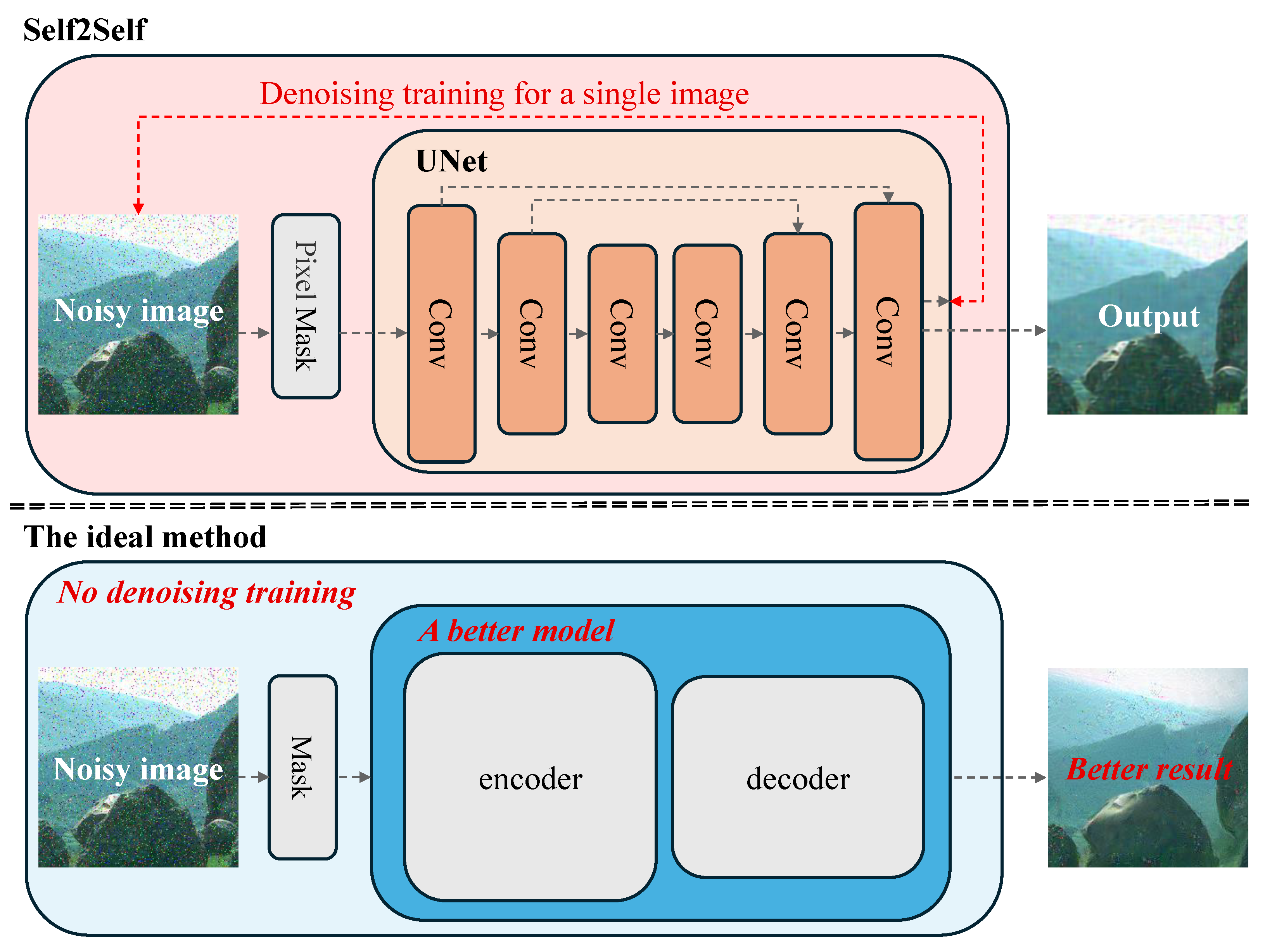
27] introduced a self-supervised learning method named Self2Self, training only with input noisy images through Bernoulli sampling instance pairs and using dropout techniques during training, addressing the issue of insufficient noise instances for training in practical application scenarios. Mansour and Heckel [28] proposed an efficient image denoising method called Zero-Shot Noise2Noise, which does not require any training data or knowledge of noise distribution, addressing the issue of insufficient noise instances for denoising in practical applications. These methods lack extensive dataset training, theoretically limiting their performance compared to supervised learning.
The Deep Image Prior (DIP) method [29] can achieve denoising by exploiting the differences between noise and image recovery difficulty. Ulyanov et al. [29] proposed the DIP method. This method does not rely on extensive training with clean-noise pairs. Instead, it leverages a randomly initialized convolutional neural network. The inductive bias of the network structure naturally adapts to the low-complexity characteristics of the image. This adaptation makes it challenging to fit high-frequency noise. This method has used the network structure’s inherent characteristics to differentiate between noise and signal, avoiding noise distribution bias and enabling image denoising without extensive training data. Due to the limitation of single-image processing, these methods are resource-intensive and generally less effective in denoising.
Some studies not only attempt to train models on Gaussian noise but also perform well on other types of noise. Chen et al. [30] proposed a training method forcing the network to focus more on image content rather than noise by masking, thus improving generalization performance. However, in practical tests, these algorithms still perform poorly under unseen high-intensity noise, making effective denoising more difficult.
In recent years, the potential of pretrained models has gained significant attention in the field of image processing [31,32,33,34,35]. Liao et al. [36] proposed an innovative image quality assessment method that evaluates perceptual degradation by comparing deep network feature distributions, without the need for additional training. This approach not only significantly improves evaluation efficiency but also effectively captures quality changes that are consistent with the human visual system. In this study, we similarly adopt the feature extraction capabilities of pretrained models as the foundation of our denoising process. Unlike traditional denoising methods that rely on training with specific noise types or intensities, pretrained models provide stronger generalization support, allowing the model to maintain robust denoising performance even when encountering unseen noise. This generalization capability enables the handling of complex noise, making it suitable for remote sensing images.
In the field of image denoising, enhancing the generalization capability of models is the primary challenge we aim to address. Masked Denoising (MD) [30] is a denoising algorithm that focuses on improving the generalization performance of models, which aligns closely with the problem we are tackling. MD suggests that pixel-level masking can effectively enhance the model’s generalization ability, while we believe that block-level masking can also provide similar generalization benefits. Based on this insight, we choose MD [30] as the main comparison for evaluating the generalization performance of denoising algorithms in the subsequent analysis.
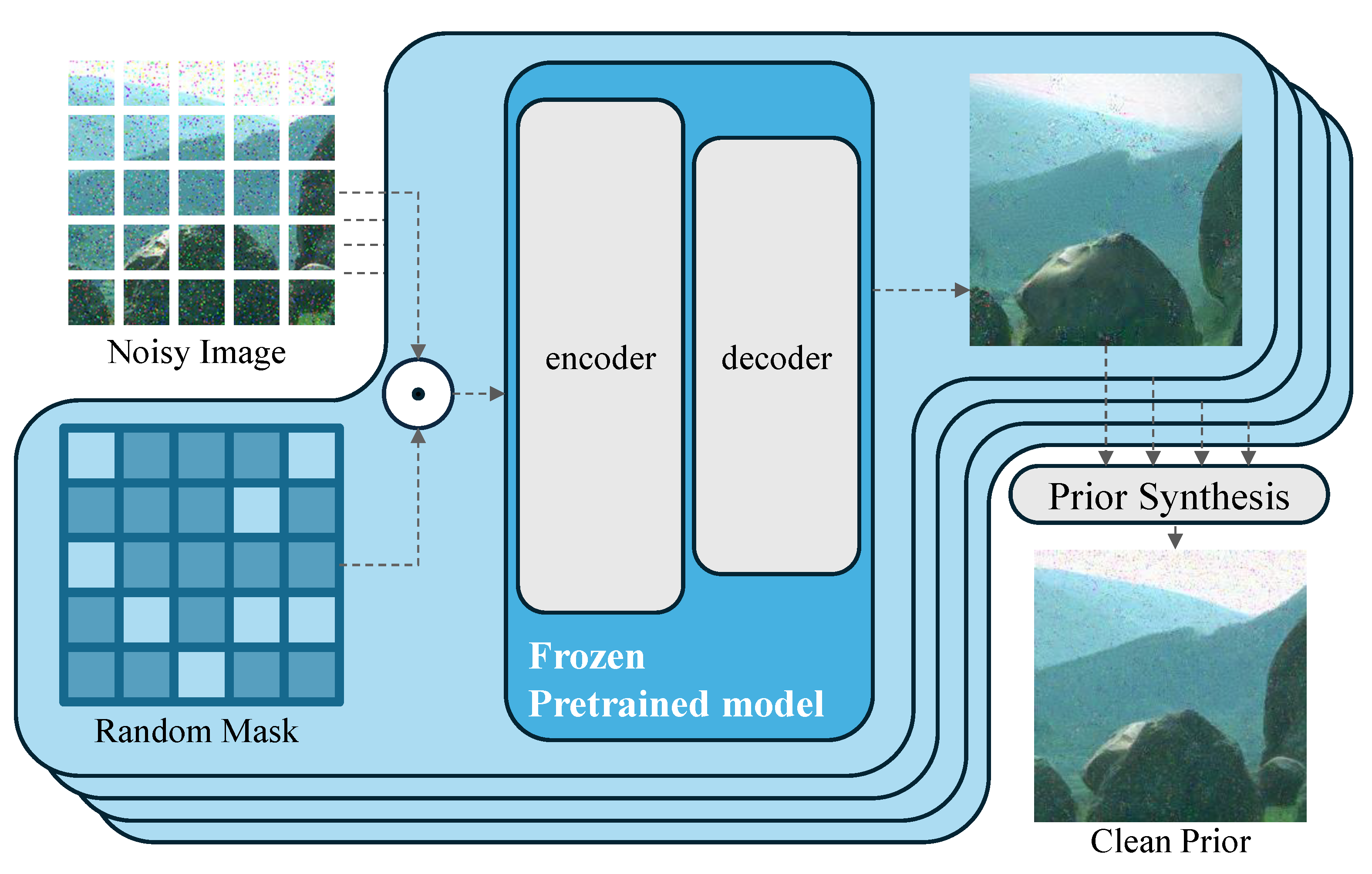
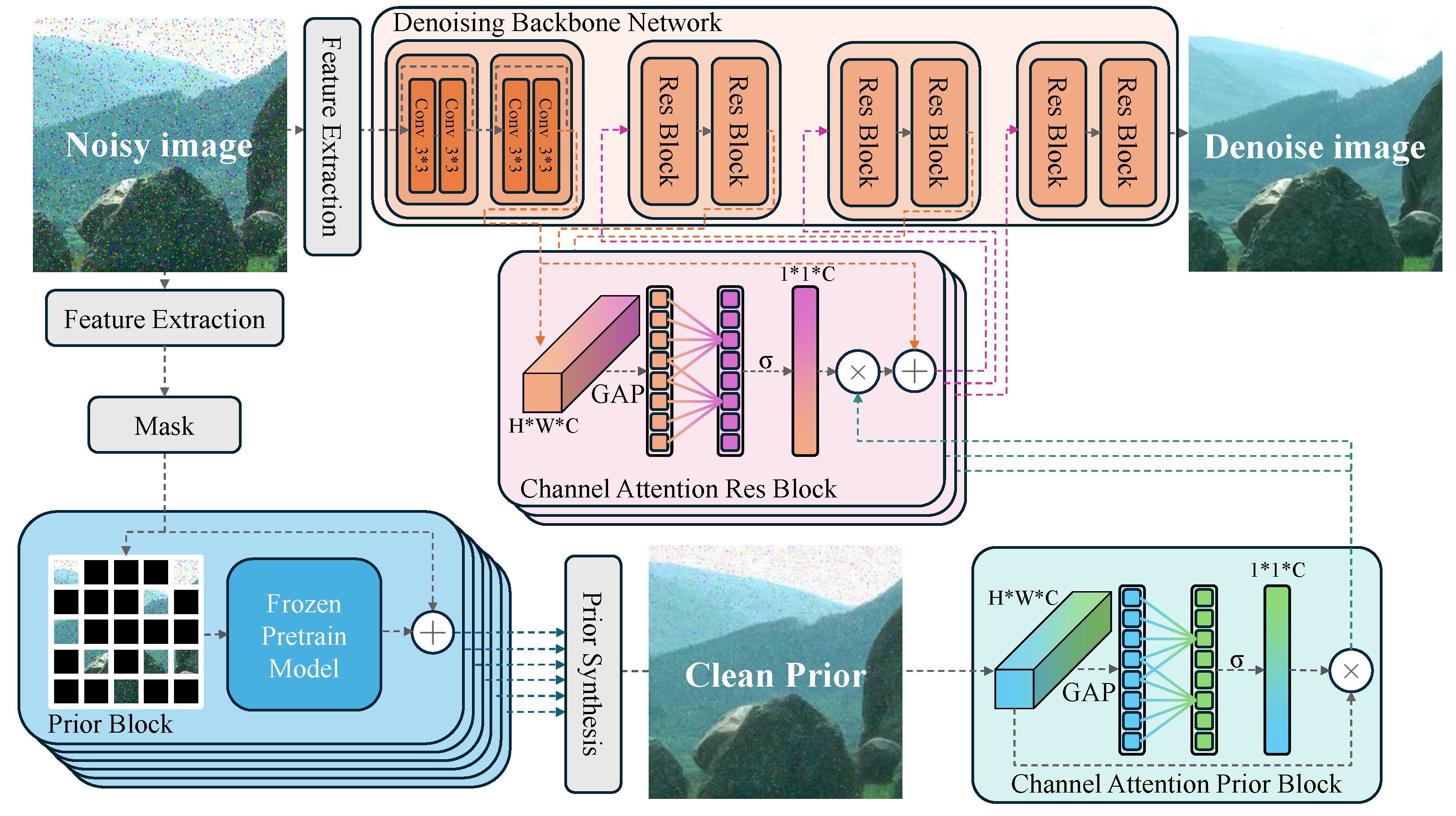
We intend to address the generalization issue in image denoising by proposing the Masked Autoencoder (MAE) pretraining method [37], which endows the model with the ability to extract image semantics. Similar to DIP [29], we can exploit the difference between noise and image semantic recovery to achieve preliminary denoising. The MAE-recovered image content tends to be semantically more inclined, allowing us to incorporate the strong image feature extraction capabilities of MAE self-supervised training into the existing algorithms. We use the features extracted by MAE [37] for coarse image reconstruction, followed by a more fine-grained convolutional network to further separate noise and restore image details.
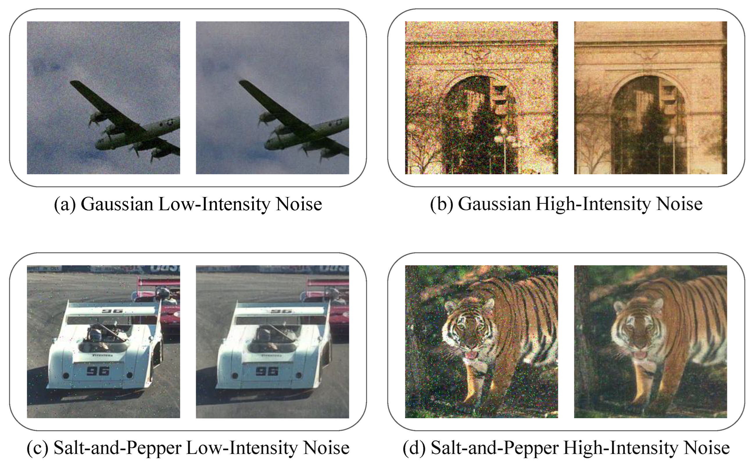
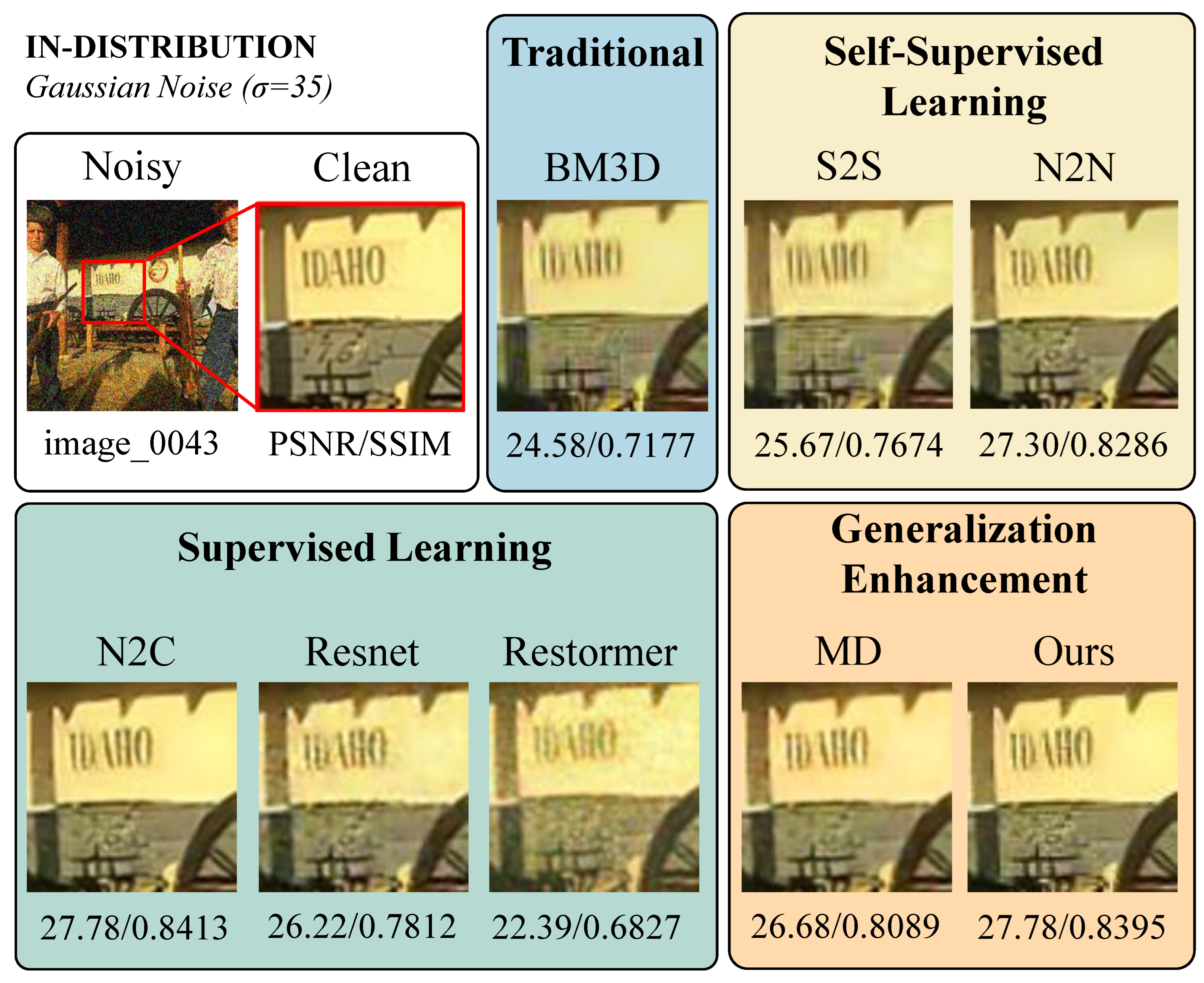
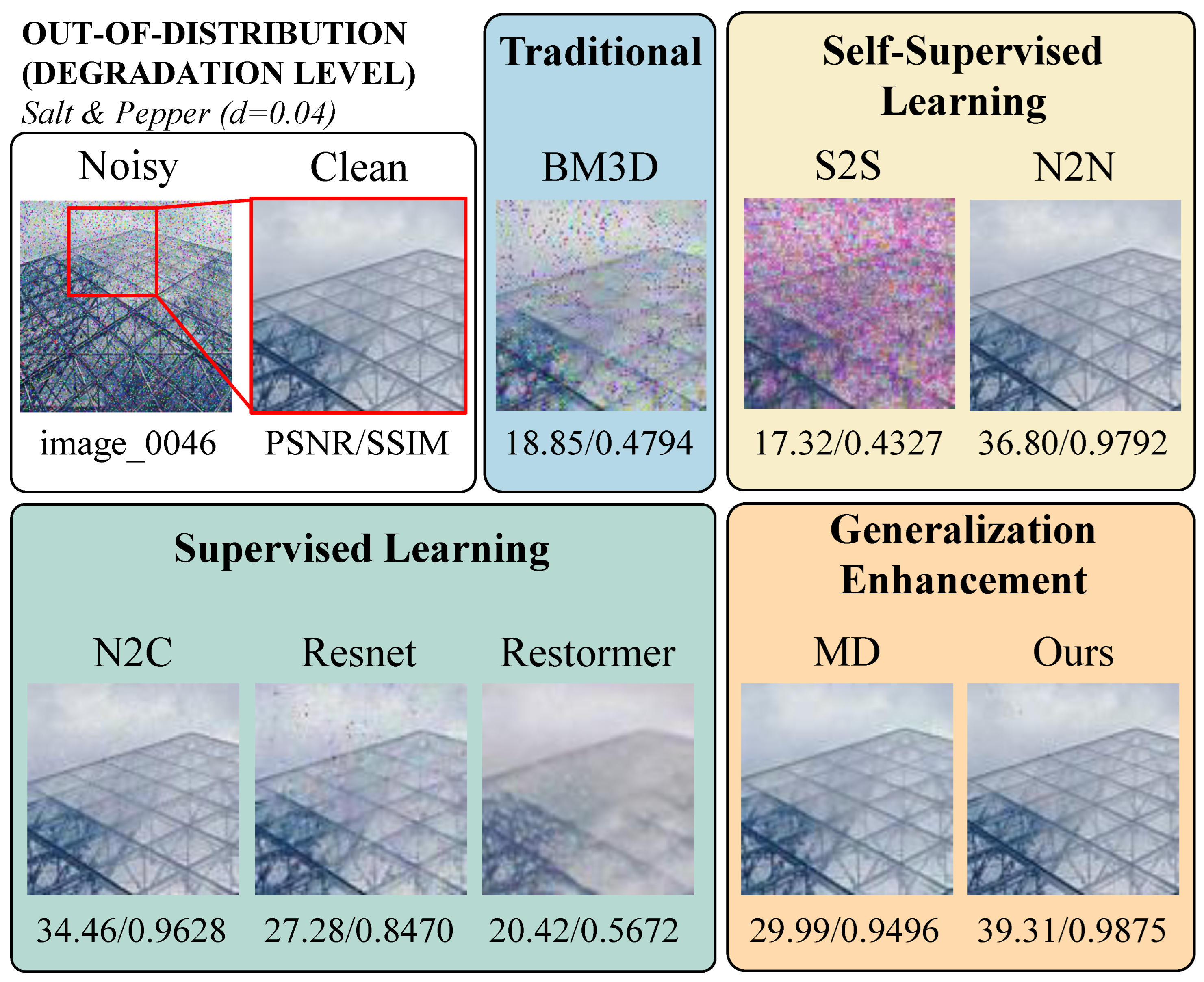
As a result, our method demonstrates superior denoising performance compared to the Masked Denoising (MD) [30], both in in-distribution and out-of-distribution scenarios. As shown by the in-distribution denoising results in Figure 1, our method produces cleaner texture restoration on the hat, whereas the MD algorithm [30] introduces noticeable color artifacts. The out-of-distribution denoising results in Figure 1 further illustrate that our method provides sharper detail recovery on the tree compared to MD [30].
Our main contributions are as follows:
  • We leverage a Masked Autoencoder (MAE) pretrained on clean images to extract semantic priors without explicit denoising training. This enhances the model’s generalization across diverse noise distributions, improving robustness in both in-distribution and out-of-distribution noise scenarios.
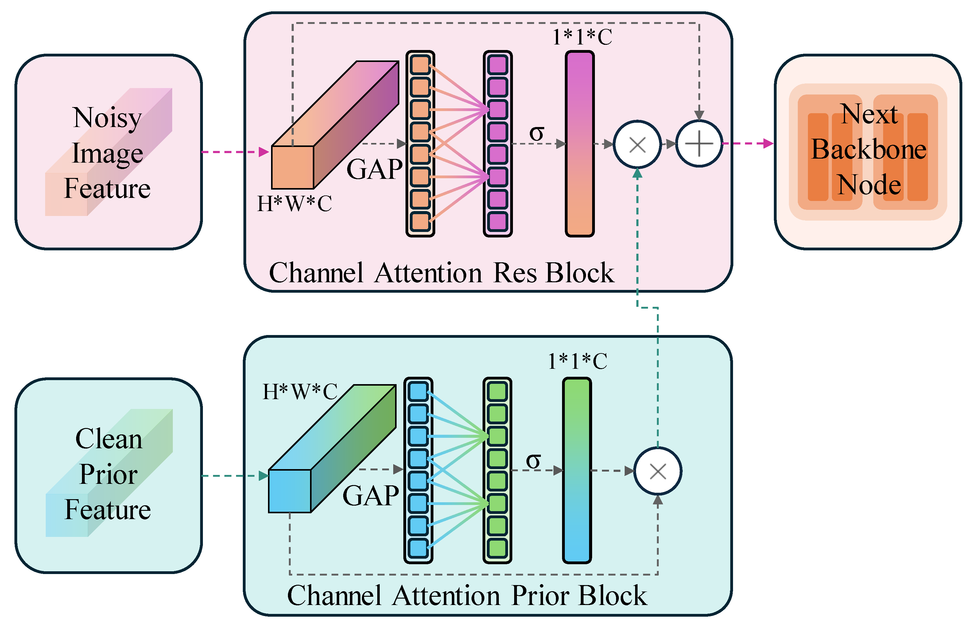
  • We introduce an asymmetric training framework, where one branch learns clean image priors from a pretrained model, while the other undergoes supervised noisy–clean training. To effectively merge these features, we design a symmetric channel attention mechanism, ensuring optimal fusion of pretrained priors and supervised features.
  • Our approach balances denoising effectiveness and computational efficiency, making it well-suited for resource-limited environments such as edge computing. Extensive experiments across multiple noise types and real-world datasets demonstrate that our method achieves state-of-the-art performance while maintaining fast inference speed.
The code is available at: https://github.com/zxz686/clean-prior-without-denoising-training (accessed on 5 March 2025).

1.1. Related Work

1.1.1. Classical Image Denoising Algorithms

Supervised learning-based image denoising algorithms typically rely on large datasets of noisy-clean image pairs to train a model that learns the denoising mapping function [38,39,40]. Usually, let the input noisy image be y, the corresponding clean image be x, and the noise be n. The relationship between the noisy image and the clean image is y = x + n . The goal of supervised learning methods is to learn a mapping function f θ such that f θ ( y ) x , where θ represents the parameters of the neural network. To optimize f θ , these algorithms need to define a loss function L and optimize it over a large number of samples.
DnCNN is a classic image denoising model based on convolutional neural networks. This model improves denoising performance by learning the residual mapping, i.e., predicting the noise n rather than directly predicting the clean image x [17].
FFDNet enhances model adaptability and flexibility by adding a noise level map as input in addition to the noisy image [18].
HPDNet leverages a PID controller combined with an attention-based recursive network to achieve adaptive feature control, encouraging the network to extract more discriminative features and enabling faster and more robust denoising [41].
Self2Self is an unsupervised image denoising method based on self-supervised learning. It achieves unsupervised image denoising through mask training. Specifically, Self2Self uses a random mask to cover part of the input image, and trains the network to predict the covered parts based on the uncovered parts. This way indicates the network can learn some inherent structures and patterns of the image without the need for clean images [16,27]. The mask training approach of Self2Self significantly inspires our research.
Deep Image Prior (DIP) [29] is a pretraining-free image denoising method, which reveals the difference in the ability of neural networks to fit low-frequency and high-frequency information. DIP [29] directly optimizes the network parameters to make its output as close as possible to the input image, thus achieving denoising. This method demonstrates that deep neural networks can capture the structural information of images well, even without any training data. The core idea of DIP is that the network structure itself has a powerful expressive capability to recover clean images from noisy ones [29].

1.1.2. Generalizable Image Denoising

Chen et al. [30] proposed the MD algorithm, i.e., a supervised learning method based on mask training. This method uses Gaussian noise with a variance of 15 during training and also performs well on various other noise types, demonstrating strong generalization capabilities. The core idea of the MD algorithm [30] is to make the model more focused on restoring the image by using mask training, thus achieving excellent denoising performance under different noise conditions. Specifically, the MD algorithm [30] adds a mask to a certain layer of the Swin-Transformer network based on supervised learning, which can be expressed as:
f φ ( y i ¯ m a s k i ) ,
where y i ¯ represents the features of the input noisy image from the network, mask i is the corresponding random mask, ⊙ represents element-wise multiplication, and f φ represents a certain layer in the network. Through this training method, the MD algorithm not only performs well under training noise conditions, but also maintains good denoising performance under different noise conditions [30].

1.1.3. Pretrained Models in Image Processing

Pretrained models have shown excellent performance in the field of image processing in recent years, especially in natural image understanding and generation.
MAE [37] is a self-supervised learning method based on mask training, initially used for image restoration tasks. MAE trains the network to recover masked parts of the input image, thereby learning both global and local features of the image.
One significant advantage is that pretrained models like MAE [37] can significantly reduce the cost of training on large datasets. By utilizing the pretrained MAE models [37], we can directly apply them to downstream tasks such as image denoising without training on large datasets from scratch. This not only saves computational resources but also accelerates the research and development process.
MAE [37] is primarily used for feature extraction in advanced vision tasks such as image classification, object detection, and image segmentation. In these tasks, MAE [37] significantly improves model performance through its powerful feature extraction capabilities. However, its application in low-level vision tasks such as image denoising has not been widely explored.
Although MAE [37] has achieved success in advanced vision tasks [42,43,44], we believe it also has great potential in low-level vision tasks, such as image denoising.

2. Materials and Methods

2.1. Motivation

In extreme scenarios where no denoising datasets are available, Self2Self [16] provides a solution by utilizing a single noisy image and an untrained neural network for denoising. Self2Self [16] achieves this by randomly masking small regions of the noisy image and using the remaining pixels to predict the masked regions. Through iterative learning to reconstruct the masked regions, Self2Self [16] successfully denoises a single image. However, this approach has significant computational limitations: even with lightweight models like UNet, processing a single 256 × 256 color image requires nearly an hour. Moreover, the trained model is highly specific to the input image, rendering its parameters unusable for other images.
In view of the limitations of Self2Self [16], as illustrated in Figure 2, an ideal denoising method should address the computational overhead associated with per-image training. With advances in deep neural networks, it should be feasible to employ more sophisticated architectures, overcoming the reliance on small models imposed by time constraints. To this end, we propose replacing the per-image training process in Self2Self [16] with pretrained models trained on noise-free images. Pretrained models developed for advanced vision tasks, such as MAE (Masked Autoencoder) [37], can be leveraged for this purpose. Our findings indicate that MAE [37], as a model for clean image reconstruction, inherently possesses denoising capabilities. As an image information extractor, MAE can effectively separate noise from semantic information, preserving the image content in noisy images and bringing them closer to clean images. Experimental results, as shown in Figure 3, demonstrate that the pretrained MAE model achieves significant denoising performance across various noise types and intensities.
Algorithms leveraging pretrained models fundamentally differ from traditional supervised image denoising methods. Supervised denoising tasks inherently induce a bias toward specific noise types based on the training dataset. For instance, DnCNN [17], trained on Gaussian noise with a variance of 15, is highly effective for that specific noise type but requires retraining on a new dataset when the noise type changes. In contrast, pretrained models based on non-denoising tasks are not tied to any specific noise type, making them well-suited for developing highly generalized image denoising algorithms.
To enhance the generalization capabilities of denoising models, Chen et al. [30] proposed a supervised learning method utilizing mask training, focusing exclusively on Gaussian noise with a variance of 15. While this method demonstrated satisfactory performance on other noise types, its effectiveness diminished under high-intensity noise conditions, as observed in practical tests [30]. To address these limitations, we propose an asymmetric denoising approach that leverages both supervised learning (trained on noisy–clean image pairs) and pretrained models from non-denoising tasks. By integrating the image reconstruction capabilities of models such as MAE [37] with our backbone network, we achieve strong generalization and effective denoising under diverse noise conditions.

2.2. Clean Image Prior with MAE Pretraining

To enhance the effectiveness of image denoising, we utilize the MAE pretrained model, which excels in clean image recovery tasks. Although the MAE [37] does not directly perform image denoising and has not been trained for denoising, our experiments indicate that it possesses inherent denoising capabilities. We aim to leverage this by designing a Prior Block to provide prior information for our denoising method. As shown in Figure 4, our approach involves applying multiple randomly generated masks to the noisy image and inputting it multiple times into the MAE pretrained model [37] to obtain MAE recovery results. These results are then synthesized using Prior Synthesis to form a clean prior image. Our clean prior image maintains the same size and channels as the input, facilitating the generation of pixel-by-pixel corresponding features to the original image dimensions. This integration allows us to effectively incorporate this information into the backbone network for noise removal. Specifically, for each image processed by the pretrained model, we supplement the input image into the output’s non-masked parts, yielding a complete image. Due to the evident grid effects between the generated masked parts and the parts filled with the original image, we perform this operation multiple times on a single image to obtain a smooth result. The formula is as follows:
p r i o r = 1 N i = 1 N M A E ( m a s k i y ) + ( 1 m a s k i ) y .

2.3. Denoising Network Design (Backbone Network)

Image denoising aims to restore a clean image from a noisy input, which requires preserving essential semantic information while suppressing noise-induced distortions. Our analysis based on the Frechet Inception Distance (FID) [45] metric (Table 1) reveals that as noise intensity increases, the Clean Prior generated by the Clean Prior Block retains more semantic information than the noisy input. However, under low noise conditions, the semantic gap between the noisy image and the Clean Prior is minimal. This observation suggests that the backbone network must dynamically balance the reliance on features extracted from the noisy input and those from the Clean Prior Block to ensure optimal denoising performance across different noise levels. Furthermore, to preserve per-pixel information while preventing spatial distortions during feature fusion, we adopt a channel-only attention mechanism. This design ensures that the attention mechanism focuses on enhancing the most informative feature channels, which avoids unintended influences of neighboring pixels and enhances the robustness of the feature fusion process.
For the clean image priors obtained earlier, we design an attention mechanism to effectively extract these priors within the backbone network. To reduce the computational cost of the attention mechanism, we apply attention processing in the channel dimension of the features. This approach is similar to the one used in the Hybrid Domain Attention Network (HDANet) [46], which also reduces computational complexity by efficiently processing features in both spatial and channel domains. By focusing on channel-wise attention, we significantly reduce the computational overhead, making it more suitable for resource-constrained edge computing environments.
Specifically, as illustrated in Figure 5, we adopt a symmetric channel attention mechanism where one-half of the module processes features derived from the backbone network (supervised by the denoising task), while the other half handles clean image priors produced by a pretrained model in a non-denoising task. Since the prior module has already extracted contextual information around each pixel, channel attention precisely meets our needs. This approach is similar to that seen in the ETLSH-YOLO method [47], where efficient integration of model components ensures edge computing efficiency, enabling superior performance on resource-constrained devices. First, a 1 × 1 convolution layer converts the clean prior image from the MAE [37] (dimension H × W × 3) into a feature map (dimension H × W × C). Then, global average pooling (GAP) compresses the feature map (dimension H × W × C) into a 1 × 1 × C vector. This vector is processed by a 1D convolution-based channel attention mechanism (ECA), where the kernel size is dynamically determined based on the number of input channels. This enables adaptive channel weighting without the need for fully connected layers. The computed attention scores are then passed through a sigmoid activation function to obtain the final channel attention weights.
A t t e n t i o n l = s i g m o i d ( L C ( G A P ( f e a t u r e l ) ) ) .
For a certain layer in the backbone network, we compute channel attention similarly to the clean image priors, but without sharing parameters with the clean image priors or other layers of the backbone network.
A t t e n t i o n p r i o r = s i g m o i d ( L C ( G A P ( f e a t u r e p r i o r ) ) ) .
The above equations exhibit a symmetric structure in the feature fusion process. Specifically, Equations (3) and (4) are structurally identical, ensuring that both noisy image features and clean prior features undergo the same transformation process before fusion. Intuitively, this mechanism functions like a selective filter that emphasizes the most relevant feature channels while suppressing less informative ones. By computing separate attention scores for noisy image features and clean priors, our model ensures that the backbone network receives a well-balanced combination of both, enhancing the denoising performance without introducing unnecessary artifacts. In the backbone network, the features at each attention calculation point are processed with the following formula and used as input for the next layer.
f e a t u r e l = f e a t u r e l + f e a t u r e p r i o r A t t e n t i o n l A t t e n t i o n p r i o r .
This ensures that both feature sources contribute proportionally to the final representation, maintaining the structural integrity of the denoised image.
The algorithm framework, as illustrated in Figure 6, shows the overall structure of our proposed method. As our prior module has already extracted information around pixels to generate clean image priors, the backbone network theoretically does not need to employ the self-attention mechanism of the Swin-Transformer. Therefore, we use a convolutional network with skip connections as the backbone network. Specifically, we use a ResNet-based [48] architecture consisting of 12 convolutional layers, structured as 6 residual blocks, each containing two 3 × 3 convolutional layers and a skip connection.
In the backbone network, every two residual blocks form a group, resulting in 6 groups of residual blocks. Starting from the second group, the input to each group is determined jointly by an independent Channel Attention Residual Block (CARB) and the output from the Channel Attention Prior Block (CAPB). Each residual block is followed by an Efficient Channel Attention (ECA) module, yielding a total of 6 ECA modules in the network.
Then, global average pooling (GAP) compresses the feature map (dimension H × W × C) into a 1 × 1 × C vector. This vector is processed by a 1D convolution-based channel attention mechanism, where the kernel size is dynamically determined based on the number of input channels. This enables adaptive channel weighting without the need for fully connected layers. The computed attention scores are then passed through a sigmoid activation function to obtain the final channel attention weights.
To facilitate channel attention computation and maintain feature information, we keep the feature dimensions in the backbone network as H × W × C, where H and W are the height and width of the input image, respectively. The feature dimension C is fixed at 64 across all convolutional layers and remains unchanged throughout the network.
In summary, our approach embodies an asymmetric structure where one part of the model, the Clean Prior Block, is derived from a pretrained model that has never been trained on noisy images, while the backbone network undergoes direct supervision on noisy-clean image pairs. This asymmetry ensures that the network benefits from both pretrained semantic priors and task-specific denoising supervision.

3. Experiments

3.1. Datasets and Experiment Setup

Training Settings: In our training process, we utilize the masked denoising (MD) algorithm [30] as the baseline, adopting similar training settings. To ensure a fair comparison with the MD method, we use the same clean image datasets: DIV2K [49], Flickr2K [50], BSD500 [51], and WED [52]. These datasets are also commonly used in other image denoising methods, such as the SwinIR image enhancement algorithm [53]. For the use of the Masked Autoencoder (MAE) [37], the input image size is set to 224 × 224 × 3. We use the Adam optimizer [54] with parameters β 1 = 0.9 and β 2 = 0.99 to minimize the L 1 pixel loss. The initial learning rate is set to 1 × 10 4 , and the batch size is 64. The training process is divided into Gaussian noise training and mixed noise training. For Gaussian noise training, Gaussian noise with a variance σ = 15 is used, while the mixed noise training involves various noise types with the following parameters:
  • Gaussian Noise: Standard deviation σ uniformly random in the range of [15, 35];
  • Speckle Noise: Noise intensity uniformly randomin the range of [0.01, 0.1];
  • Poisson Noise: Scale factor uniformly random in the range of [1, 5];
  • Salt-and-Pepper Noise: Noise density uniformly random in the range of [0.002, 0.02].
Testing Dataset: To evaluate the generalization capability of our method, we conduct experiments on the CBSD68 dataset [55], a widely used benchmark for image denoising. Unless otherwise specified, all reported test results are obtained on CBSD68.
Evaluation Metrics: We chose PSNR, SSIM [52], and LPIPS [56] as evaluation metrics because PSNR measures pixel-wise fidelity, SSIM [52] captures structural similarity, and LPIPS [56] provides a perceptual evaluation that aligns with human visual perception. Together, these metrics offer a comprehensive assessment of both objective and perceptual image quality.

3.2. Comparison of Models Trained on Gaussian Noise with Variance σ = 15

The results in Table 2 are derived when models are trained on Gaussian noise with σ = 15 . In this table, we have tested the models on the training noise level of σ = 15 and also on higher noise levels of σ = 25 , σ = 35 , and σ = 50 to evaluate their generalization performance. The top three methods listed in the table are traditional supervised learning approaches without any specific generalization performance design. ResNet [48] is a convolutional neural network algorithm that uses residual connections. Since the original Resnet performs poorly on denoising tasks, we modified its hyperparameters to adapt it to image denoising. SwinIR [53] is an image restoration model based on the Swin Transformer. Noise2Clean (N2C) is a supervised learning algorithm that uses clean images for supervision and shares the same backbone network as Noise2Noise (N2N) [26]. In contrast, the bottom three methods incorporate generalization strategies: while Noise2Noise (N2N) [26] is not specifically designed for generalization, it uses noisy images instead of clean supervision, which can improve generalization performance; the authors of MD [30] claim that their algorithm, trained on Gaussian noise with σ = 15 , performs well on other types of noise; the last method is our proposed algorithm.
As shown in the experimental results in Table 2, all algorithms were trained on Gaussian noise with a standard deviation of 15. Although MD [30] and our method, which are designed specifically for generalization, did not achieve the best results at σ = 15 , they outperformed the other methods in out-of-distribution noise levels of σ = 25 , σ = 35 , and σ = 50 by achieving the first or second-best performance in terms of PSNR, SSIM [52], and LPIPS [56]. This demonstrates that algorithms designed to enhance generalization tend to perform better at out-of-distribution noise levels than other algorithms.

3.3. Denoising Results Within the Distribution of Mixed Noise Dataset

In practical scenarios, it is unrealistic to rely on models trained solely on a single noise type to handle unknown noise. Instead, we aim for models that are exposed to a variety of noise types during training and perform well on these noises. Table 3 presents the performance of different models trained on multiple noise types to evaluate their effectiveness across these noise conditions.
The performance of various algorithms under different noise conditions is compared in Table 3. Among these, BM3D [57] is included as a representative non-neural network algorithm. Since BM3D [57] requires manual input of the noise standard deviation, some studies [58] have proposed methods for automatic noise estimation. To ensure fair comparison across different noise types, we incorporated a simple automatic noise estimation module. Notably, Self2Self (S2S) [27] is a unique neural network-based algorithm that does not involve a training process, and it is included for comparative purposes. Algorithms marked with “*” denote models released by their respective authors. The bottom five algorithms in the table are all trained on the same dataset, ensuring consistency in training conditions.
According to the results in Table 3, our method achieves the best scores in PSNR and LPIPS [56] and the second-best score in SSIM [52] on Gaussian noise with σ = 15 . On Gaussian noise with σ = 25 and σ = 35 , our method achieves the second-best scores in both PSNR and SSIM [52]. The bottom three noise types in Table 3 correspond to the highest noise levels within the distribution. In speckle noise, Poisson noise, and salt-and-pepper noise, our method just achieved the best scores in PSNR, SSIM [52], and LPIPS [56].
In summary, our method achieves either the best or second-best scores for most noise types in the distribution with mixed noise training, and demonstrates the best performance under the strongest in-distribution noise levels.

3.4. Denoising Results for Models on Out-of-Distribution Noises with Models Trained on Mixed Noise Dataset

It is insufficient for an algorithm to perform well only on previously seen noise types. To thoroughly evaluate the generalization capabilities, the algorithm must also demonstrate robust performance across various degradation types and levels. Table 4 presents the results of the algorithms under different degradation levels, while Table 5 shows the performance on noise types that differ from those encountered during training.
As shown in Table 4, our algorithm achieves the best scores in all three metrics for Gaussian noise with lower degradation levels at σ = 5 and σ = 10 . At the higher degradation level of Gaussian noise with σ = 50 , our algorithm obtains the best score in PSNR and the second-best score in SSIM [52]. Salt-and-pepper noise, speckle noise, and Poisson noise in Table 4 represent out-of-distribution noise with higher degradation levels. For salt-and-pepper noise, our algorithm achieves the best scores in PSNR, SSIM [52], and LPIPS [56], with PSNR leading by nearly 4 dB compared to the second-best method. For speckle noise and Poisson noise, our algorithm ranks second in PSNR and SSIM [52] for speckle noise, and achieves the best scores in both PSNR and SSIM [52] for Poisson noise.
As shown in Table 5, our algorithm achieves the highest PSNR and SSIM [52] scores for Constant Poisson on λ = 9 and λ = 40 , and the second-best PSNR score for Constant Poisson on λ = 20 .
Overall, these results demonstrate that our algorithm exhibits strong generalization capabilities across both in-distribution and out-of-distribution noise types and degradation levels.

4. Discussion

4.1. Visual Results and Analysis

To visually demonstrate the superior performance of our proposed method, we select three sets of images to show the denoising results under in-distribution, out-of-distribution (noise type), and out-of-distribution (noise intensity) scenarios. The comparative methods include our generalization enhancement baseline MD [30], the traditional non-learning algorithm BM3D [57], self-supervised learning algorithms S2S [27] and N2N [26], and supervised learning algorithms N2C, ResNet [48], and Restormer [59].
In the first set of images (Gaussian noise, σ = 15 ), as shown in Figure 7, it is evident that our method effectively restores image details under in-distribution noise, particularly in the text region on the wall, performing on par with or slightly better than mainstream denoising algorithms. While N2C achieves high PSNR and SSIM [52] in this scenario, our method provides a clearer visual restoration.
The second set of images demonstrates the performance of the algorithms under out-of-distribution (noise intensity) conditions (Salt & Pepper noise, d = 0.04), as shown in Figure 8. Under high noise intensity, traditional and some supervised learning methods almost completely fail, with significant loss of image details. In contrast, our method restores the structural details and lines near the building’s spire with superior clarity compared to other methods, and it achieves significantly higher PSNR and SSIM [52] values, verifying the robustness of our approach to varying noise intensities.
The third set of images shows the performance under out-of-distribution (noise type) conditions (Constant Poisson noise, λ = 40 ), as shown in Figure 9. Our method excels in restoring the details of the train, with superior clarity and color preservation compared to other methods. In comparison, although N2C performs better than MD [30] in terms of metrics, it still retains noticeable noise-induced color artifacts, and the structural clarity is slightly inferior to our method. Other traditional and some supervised learning algorithms exhibit clear denoising failures.
In summary, our method not only outperforms compared to the other competing methods in quantitative metrics (PSNR and SSIM [52]), but also demonstrates significantly better visual performance, showcasing superior generalization ability and denoising effectiveness.

4.2. Multi-Noise Denoising on Remote Sensing Dataset

Remote sensing images are subject to various types of noise, including thermal noise, dark noise, and photon shot noise, which arise from the physical limitations of imaging equipment [1,60,61]. Among these, random noise is particularly challenging to eliminate through hardware. Photon noise is signal-dependent (approximated by a Poisson distribution), while other random noises often follow a combination of Gaussian distributions, adding complexity to the denoising task. To simulate the effects of multiple noise types on remote sensing images, we applied a combination of Gaussian, Poisson, speckle, and salt-and-pepper noise, with the following parameters:
  • Gaussian Noise: Standard deviation σ in the range of [0.1, 1]
  • Speckle Noise: Noise intensity in the range of [0.0009, 0.01]
  • Poisson Noise: Scale factor in the range of [5, 10]
  • Salt-and-Pepper Noise: Noise density in the range of [0.0005, 0.005]
This approach aims to mimic real-world scenarios where images are affected by multiple, simultaneous noise sources, providing a comprehensive test of our denoising algorithm’s robustness. The dataset used in this experiment was the AID [62] remote sensing dataset.
As shown in Figure 10, our method demonstrates superior visual denoising performance on multi-noise remote sensing images compared to traditional supervised learning (N2C) and the generalization-oriented MD [30] algorithm. In terms of quantitative evaluation, as presented in Table 6, our approach achieves the best results for PSNR and LPIPS [56] in the simulated denoising experiments on the AID dataset [62]. Additionally, our method attains the second-best SSIM [52] score, with only a 0.0036 difference from the top-performing MD [30] method.

4.3. Ablation Experiment

To comprehensively validate the effectiveness of each component in our method and the impact of different backbone networks, we conduct a series of ablation experiments, and specifically analyze the influence of clean image priors generated by the Masked Autoencoder (MAE) [37] and the Channel Attention Mechanism (CAtt) on denoising performance. Additionally, we explore the effect of different backbone networks on the overall performance.
First, we analyze the impact of the clean image priors generated by MAE [37] and the Channel Attention Mechanism (CAtt) on denoising performance. Table 7 shows the experimental results under different noise types (Gaussian noise and Salt & Pepper noise), using PSNR, SSIM [52], and LPIPS [56] as evaluation metrics.
The results in Table 7 indicate that both the clean image priors generated by MAE [37] and the Channel Attention Mechanism (CAtt) significantly enhance denoising performance. Specifically, under both Gaussian noise and Salt & Pepper noise, the model combining MAE [37] and CAtt (ID 1 and ID 4) achieves the best results in terms of PSNR, SSIM [52], and LPIPS [56].
These findings demonstrate that the clean image priors generated by MAE [37] effectively improve denoising performance, while the introduction of the channel attention mechanism further enhances the effectiveness of the model.
Next, we compare the performance of various backbone network architectures in the denoising task. Table 8 presents the performance of our method with different backbone networks.
Our preliminary module extracts the surrounding information of pixels to generate clean image priors, thus the backbone network theoretically does not need to employ the self-attention mechanism of the Swin-Transformer (Swin-T) [63]. Therefore, using a convolutional network with skip connections, such as ResNet [48] as the backbone network, is more appropriate. The experimental results indicate that employing ResNet [48] as the backbone network outperforms the baseline MD algorithm [30] in terms of PSNR and LPIPS [56], and slightly surpasses the Swin-Transformer [63] version in SSIM [52].

4.4. Computational Cost and Edge Deployment

To evaluate the computational efficiency of our method, we conduct a comparative analysis of inference time, model parameters, and FLOPs with other state-of-the-art methods, including SwinIR [53] and Restormer [59]. The computational cost is a critical aspect in evaluating the feasibility of deploying denoising models in resource-constrained environments, such as edge devices.
Table 9 presents a detailed comparison of different models based on key computational metrics. Our method achieves the lowest inference time among all evaluated models, despite incorporating an additional pretrained MAE component. The high efficiency stems from the lightweight denoising network, which minimizes the computational burden while leveraging MAE’s pretrained features for enhanced performance.
Compared to SwinIR [53], which requires 422 GFLOPs for inference, our method significantly reduces computational complexity, utilizing only 44.52 GFLOPs for the denoising network. Additionally, our method outperforms Restormer [59] in inference time while maintaining comparable computational requirements. The combination of a lightweight denoising backbone and a pretrained MAE model [37] allows our approach to balancing computational cost and performance effectively. However, a pretrained MAE model does introduce an additional computational burden. As shown in Table 9, processing a single 224 × 224 color image with the MAE prior module takes approximately 0.1400 s, which is 10 times the 0.0140 s required by the denoising backbone. While our method remains computationally efficient compared to existing transformer-based approaches, this overhead could be a limitation in extremely resource-constrained environments. Future work could explore optimizing the pretrained feature extraction process to further reduce latency.
Furthermore, we assess the suitability of our method for edge computing scenarios by analyzing its computational footprint relative to available hardware constraints. Our approach exhibits a substantial reduction in parameter count compared to SwinIR [53] and Restormer [59], making it more feasible for deployment on edge devices with limited memory and computational capacity. The reduced inference time of the model also suggests its potential for real-time denoising applications in edge computing environments.
In addition, we consider an alternative scenario where computational resources are relatively abundant while the system needs to handle multiple types of noise simultaneously. In such cases, the training cost of MAE does not contribute to the deployment overhead, making it a viable option for edge applications with moderate resource availability. Unlike SwinIR [53] and Restormer [59], which require separate models for different noise distributions, our method demonstrates strong generalization capability. This eliminates the need to train multiple models, significantly reducing the training cost and the number of deployed models. Consequently, our approach not only minimizes computational resources during training but also optimizes storage and inference efficiency in real-world applications.
Although transformer-based methods like Restormer [59] provide efficient self-attention mechanisms, their relatively large model sizes impose additional memory constraints. Our model addresses this limitation by integrating a lightweight denoising backbone with an efficient pretrained MAE model [37], maintaining competitive performance while optimizing computational efficiency. The results highlight that our approach achieves an effective trade-off between computational cost and performance, making it well-suited for real-world edge deployment scenarios, particularly in environments where handling multiple noise types is essential.

5. Conclusions

In this paper, we have proposed a denoising framework that leverages clean image priors from pretrained models (without denoising-specific training) and demonstrated its effectiveness in enhancing the generalization ability of deep-learning-based image denoising. By utilizing the powerful feature extraction capabilities of models such as MAE [37], our approach integrates semantic priors into the denoising process, significantly improving performance in diverse noise conditions. Experimental results confirm that our method outperforms baseline models in both in-distribution and out-of-distribution noise settings, showcasing its adaptability across different noise distributions.
A key strength of our design lies in its ability to balance asymmetry and symmetry within the denoising framework. Asymmetry arises from the dual training objectives: one component of the model learns feature representations from clean images via a pretrained network, while the other is trained through supervised learning with noisy-clean pairs. Symmetry is achieved through an efficient fusion mechanism that structurally integrates pretrained priors and supervised features, enhancing denoising quality while maintaining computational efficiency.
Beyond denoising performance, our method is particularly well-suited for real-world edge computing applications, where resource constraints necessitate an optimal trade-off between model complexity and inference speed. As detailed in the Computational Cost and Edge Deployment section, our model achieves a significant reduction in inference time and computational overhead compared to SwinIR [53] and Restormer [59]. The lightweight denoising network enables real-time processing on edge devices, while the use of pretrained priors ensures strong generalization without requiring multiple models for different noise types. This makes our approach particularly attractive for applications such as remote sensing, environmental monitoring, and embedded vision systems, where computational efficiency is critical.
While our method effectively integrates pretrained priors for image denoising, it has certain limitations. Since our framework leverages semantic priors extracted from clean images, it may struggle with noise patterns that exhibit strong semantic characteristics, such as structured stripe noise. In such cases, the model may have difficulty distinguishing noise from meaningful image details, potentially reducing denoising effectiveness. Future research could explore adaptive mechanisms to address this challenge, such as integrating noise modeling strategies that account for structured distortions.
Further exploration is also needed to optimize these priors for more complex imaging tasks. Future work may investigate the adaptation of our framework to specialized domains, such as night-time imaging, hyperspectral data analysis, and multimodal image restoration, where additional constraints and data characteristics play a crucial role. Additionally, the exploration of alternative self-supervised pretraining models beyond MAE could further enhance the denoising capabilities and deployment efficiency of our approach. Future work may investigate the adaptation of our framework to specialized domains, such as night-time imaging, hyperspectral data analysis, and multimodal image restoration, where additional constraints and data characteristics play a crucial role. Additionally, the exploration of alternative self-supervised pretraining models beyond MAE could further enhance the denoising capabilities and deployment efficiency of our approach.
By demonstrating both strong denoising performance and practical deployment feasibility, our study contributes a novel solution for resource-efficient and generalizable image restoration. We believe that our findings represent a step toward real-world adoption of learning-based denoising models in constrained environments and hope to inspire future research in combining semantic priors with low-cost denoising networks for robust, scalable image restoration solutions.

Author Contributions

Conceptualization, Y.Z.; methodology, Y.Z.; software, Y.Z.; validation, Y.Z.; formal analysis, Y.Z.; investigation, Y.Z.; data curation, Y.Z.; writing—original draft preparation, Y.Z.; writing—review and editing, X.L.; visualization, Y.Z.; supervision, X.L.; funding acquisition, X.L. All authors have read and agreed to the published version of the manuscript.

Funding

This work was supported in part by the Natural Science Foundation of Chongqing (Innovation and Development Joint Fund) under grant CSTB2023NSCQ-LZX0149, in part by the Graduate Student Research Innovation Project of Chongqing under grant CYB240031, in part by the Fundamental Research Funds for the Central Universities under grant 2023CDJKYJH019, and in part by the Natural Science Foundation of China under Grant 62302068.

Data Availability Statement

The datasets used in this study are all from open-source datasets.

Acknowledgments

We acknowledge the technical and administrative assistance provided by Chongging University.

Conflicts of Interest

The authors declare no conflicts of interest.

References

  1. Banjade, T.P.; Zhou, C.; Chen, H.; Li, H.; Deng, J.; Zhou, F.; Adhikari, R. Seismic Random Noise Attenuation Using DARE U-Net. Remote Sens. 2024, 16, 4051. [Google Scholar] [CrossRef]
  2. Wang, M.; Wang, S.; Ju, X.; Wang, Y. Image Denoising Method Relying on Iterative Adaptive Weight-Mean Filtering. Symmetry 2023, 15, 1181. [Google Scholar] [CrossRef]
  3. Byun, J.; Cha, S.; Moon, T. FBI-Denoiser: Fast Blind Image Denoiser for Poisson-Gaussian Noise. In Proceedings of the IEEE/CVF Conference on Computer Vision and Pattern Recognition, Nashville, TN, USA, 20–25 June 2021; pp. 5768–5777. [Google Scholar]
  4. Zhang, K.; Kulshrestha, S.; Metzler, C. A Scalable Training Strategy for Blind Multi-Distribution Noise Removal. IEEE Trans. Image Process. 2024, 33, 6216–6226. [Google Scholar] [CrossRef] [PubMed]
  5. Liu, Y.; Qin, Z.; Anwar, S.; Ji, P.; Kim, D.; Caldwell, S.; Gedeon, T. Invertible Denoising Network: A Light Solution for Real Noise Removal. In Proceedings of the IEEE/CVF Conference on Computer Vision and Pattern Recognition, Nashville, TN, USA, 20–25 June 2021; pp. 13365–13374. [Google Scholar]
  6. Wang, H.; Cao, J.; Guo, H.; Li, C. A Novel Self-Adaptive Deformable Convolution-Based U-Net for Low-Light Image Denoising. Symmetry 2024, 16, 646. [Google Scholar] [CrossRef]
  7. Gu, S.; Li, Y.; Gool, L.V.; Timofte, R. Self-guided network for fast image denoising. In Proceedings of the IEEE/CVF International Conference on Computer Vision, Seoul, Republic of Korea, 27 October–2 November 2019; pp. 2511–2520. [Google Scholar]
  8. Cheng, S.; Wang, Y.; Huang, H.; Liu, D.; Fan, H.; Liu, S. NBNet: Noise Basis Learning for Image Denoising with Subspace Projection. In Proceedings of the IEEE/CVF Conference on Computer Vision and Pattern Recognition, Nashville, TN, USA, 20–25 June 2021; pp. 4896–4906. [Google Scholar]
  9. Wang, Z.; Fu, Y.; Liu, J.; Zhang, Y. LG-BPN: Local and Global Blind-Patch Network for Self-Supervised Real-World Denoising. In Proceedings of the IEEE/CVF Conference on Computer Vision and Pattern Recognition, Vancouver, BC, Canada, 17–24 June 2023; pp. 18156–18165. [Google Scholar]
  10. Rahman, Z.; Aamir, M.; Bhutto, J.A.; Hu, Z.; Guan, Y. Innovative Dual-Stage Blind Noise Reduction in Real-World Images Using Multi-Scale Convolutions and Dual Attention Mechanisms. Symmetry 2023, 15, 2073. [Google Scholar] [CrossRef]
  11. Majumdar, A. Blind denoising autoencoder. IEEE Trans. Neural Netw. Learn. Syst. 2018, 30, 312–317. [Google Scholar] [CrossRef]
  12. Sil, D.; Dutta, A.; Chandra, A. Convolutional neural networks for noise classification and denoising of images. In Proceedings of the TENCON 2019-2019 IEEE Region 10 Conference (TENCON), Kochi, India, 17–20 October 2019; pp. 447–451. [Google Scholar]
  13. Cho, S.I.; Kang, S.J. Gradient prior-aided CNN denoiser with separable convolution-based optimization of feature dimension. IEEE Trans. Multimed. 2018, 21, 484–493. [Google Scholar] [CrossRef]
  14. Zhao, Y.; Li, Y.; Yang, B. Low-frequency desert noise intelligent suppression in seismic data based on multiscale geometric analysis convolutional neural network. IEEE Trans. Geosci. Remote Sens. 2019, 58, 650–665. [Google Scholar] [CrossRef]
  15. Yuan, Y.; Ma, H.; Liu, G. Partial-DNet: A novel blind denoising model with noise intensity estimation for HSI. IEEE Trans. Geosci. Remote Sens. 2021, 60, 5505913. [Google Scholar] [CrossRef]
  16. Ge, C.; Yu, X.; Li, M.; Mo, J. Self-Supervised Denoising of single OCT image with Self2Self-OCT Network. In Proceedings of the 2022 IEEE 7th Optoelectronics Global Conference (OGC), Shenzhen, China, 6–11 December 2022; pp. 200–204. [Google Scholar]
  17. Zhang, K.; Zuo, W.; Chen, Y.; Meng, D.; Zhang, L. Beyond a gaussian denoiser: Residual learning of deep cnn for image denoising. IEEE Trans. Image Process. 2017, 26, 3142–3155. [Google Scholar] [CrossRef]
  18. Zhang, K.; Zuo, W.; Zhang, L. FFDNet: Toward a fast and flexible solution for CNN-based image denoising. IEEE Trans. Image Process. 2018, 27, 4608–4622. [Google Scholar] [CrossRef] [PubMed]
  19. Aghajarian, M.; McInroy, J.E.; Muknahallipatna, S. Deep learning algorithm for Gaussian noise removal from images. J. Electron. Imaging 2020, 29, 043005. [Google Scholar] [CrossRef]
  20. Ollion, J.; Ollion, C.; Gassiat, E.; Lehéricy, L.; Corff, S.L. Joint self-supervised blind denoising and noise estimation. arXiv 2021, arXiv:2102.08023. [Google Scholar]
  21. Zhang, K.; Long, M.; Chen, J.; Liu, M.; Li, J. CFPNet: A denoising network for complex frequency band signal processing. IEEE Trans. Multimed. 2023, 25, 8212–8224. [Google Scholar] [CrossRef]
  22. Du, Y.; Han, G.; Tan, Y.; Xiao, C.; He, S. Blind image denoising via dynamic dual learning. IEEE Trans. Multimed. 2020, 23, 2139–2152. [Google Scholar] [CrossRef]
  23. Shukla, A.; Seethalakshmi, K.; Hema, P.; Musale, J.C. An Effective Approach for Image Denoising Using Wavelet Transform Involving Deep Learning Techniques. In Proceedings of the 2023 4th International Conference on Smart Electronics and Communication (ICOSEC), Trichy, India, 20–22 September 2023; pp. 1381–1386. [Google Scholar]
  24. Jebur, R.S.; Zabil, M.H.B.M.; Hammood, D.A.; Cheng, L.K.; Al-Naji, A. Image denoising using hybrid deep learning approach and Self-Improved Orca Predation Algorithm. Technologies 2023, 11, 111. [Google Scholar] [CrossRef]
  25. Li, Z.; Liu, H.; Cheng, L.; Jia, X. Image denoising algorithm based on gradient domain guided filtering and NSST. IEEE Access 2023, 11, 11923–11933. [Google Scholar] [CrossRef]
  26. Lehtinen, J.; Munkberg, J.; Hasselgren, J.; Laine, S.; Karras, T.; Aittala, M.; Aila, T. Noise2Noise: Learning image restoration without clean data. arXiv 2018, arXiv:1803.04189. [Google Scholar]
  27. Quan, Y.; Chen, M.; Pang, T.; Ji, H. Self2self with dropout: Learning self-supervised denoising from single image. In Proceedings of the IEEE/CVF Conference on Computer Vision and Pattern Recognition, Seattle, WA, USA, 13–19 June 2020; pp. 1890–1898. [Google Scholar]
  28. Mansour, Y.; Heckel, R. Zero-shot noise2noise: Efficient image denoising without any data. In Proceedings of the IEEE/CVF Conference on Computer Vision and Pattern Recognition, Vancouver, BC, Canada, 17–24 June 2023; pp. 14018–14027. [Google Scholar]
  29. Ulyanov, D.; Vedaldi, A.; Lempitsky, V. Deep image prior. In Proceedings of the IEEE Conference on Computer Vision and Pattern Recognition, Salt Lake City, UT, USA, 18–23 June 2018; pp. 9446–9454. [Google Scholar]
  30. Chen, H.; Gu, J.; Liu, Y.; Magid, S.A.; Dong, C.; Wang, Q.; Pfister, H.; Zhu, L. Masked image training for generalizable deep image denoising. In Proceedings of the IEEE/CVF Conference on Computer Vision and Pattern Recognition, Vancouver, BC, Canada, 17–24 June 2023; pp. 1692–1703. [Google Scholar]
  31. He, K.; Girshick, R.B.; Dollár, P. Rethinking ImageNet Pre-training. In Proceedings of the IEEE/CVF International Conference on Computer Vision, Seoul, Republic of Korea, 27 October–2 November 2019; pp. 4918–4927. [Google Scholar]
  32. Xie, E.; Wang, W.; Yu, Z.; An kumar, A.; Alvarez, J.M.; Luo, P. SegFormer: Simple and efficient design for semantic segmentation with transformers. Adv. Neural Inf. Process. Syst. 2021, 34, 12077–12090. [Google Scholar]
  33. Chen, H.; Wang, Y.; Guo, T.; Xu, C.; Deng, Y.; Liu, Z.; Ma, S.; Xu, C.; Xu, C.; Gao, W. Pre-trained Image Processing Transformer. In Proceedings of the IEEE/CVF Conference on Computer Vision and Pattern Recognition, Nashville, TN, USA, 20–25 June 2021; pp. 12299–12310. [Google Scholar]
  34. Xiong, Y.; Varadarajan, B.; Wu, L.; Xiang, X.; Xiao, F.; Zhu, C.; Dai, X.; Wang, D.; Sun, F.; Iandola, F.; et al. EfficientSAM: Leveraged Masked Image Pretraining for Efficient Segment Anything. In Proceedings of the IEEE/CVF Conference on Computer Vision and Pattern Recognition, Seattle, WA, USA, 16–22 June 2024; pp. 16111–16121. [Google Scholar]
  35. Mahmoudi Kouhi, R.; Stocker, O.; Giguère, P.; Daniel, S. CLOUDSPAM: Contrastive Learning On Unlabeled Data for Segmentation and Pre-Training Using Aggregated Point Clouds and MoCo. Remote Sens. 2024, 16, 3984. [Google Scholar] [CrossRef]
  36. Liao, X.; Wei, X.; Zhou, M.; Li, Z.; Kwong, S. Image Quality Assessment: Measuring Perceptual Degradation via Distribution Measures in Deep Feature Spaces. IEEE Trans. Image Process. 2024, 33, 4044–4059. [Google Scholar] [CrossRef] [PubMed]
  37. He, K.; Chen, X.; Xie, S.; Li, Y.; Dollár, P.; Girshick, R. Masked autoencoders are scalable vision learners. In Proceedings of the IEEE/CVF Conference on Computer Vision and Pattern Recognition, New Orleans, LA, USA, 18–24 June 2022; pp. 16000–16009. [Google Scholar]
  38. Tian, C.; Xu, Y.; Fei, L.; Yan, K. Deep learning for image denoising: A survey. In Genetic and Evolutionary Computing, Proceedings of the Twelfth International Conference on Genetic and Evolutionary Computing, Changzhou, China, 14–17 December 2019; Springer: Singapore, 2019; pp. 563–572. [Google Scholar]
  39. Goyal, B.; Dogra, A.; Agrawal, S.; Sohi, B.S.; Sharma, A. Image denoising review: From classical to state-of-the-art approaches. Inf. Fusion 2020, 55, 220–244. [Google Scholar] [CrossRef]
  40. Jebur, R.S.; Zabil, M.H.B.M.; Hammood, D.A.; Cheng, L.K. A comprehensive review of image denoising in deep learning. Multimed. Tools Appl. 2024, 83, 58181–58199. [Google Scholar] [CrossRef]
  41. Ma, R.; Li, S.; Zhang, B.; Li, Z. Towards fast and robust real image denoising with attentive neural network and PID controller. IEEE Trans. Multimed. 2021, 24, 2366–2377. [Google Scholar] [CrossRef]
  42. Wei, W.; Nejadasl, F.K.; Gevers, T.; Oswald, M.R. T-MAE: Temporal Masked Autoencoders for Point Cloud Representation Learning. arXiv 2023, arXiv:2312.10217. [Google Scholar]
  43. Sun, L.; Lian, Z.; Liu, B.; Tao, J. Mae-dfer: Efficient masked autoencoder for self-supervised dynamic facial expression recognition. In Proceedings of the 31st ACM International Conference on Multimedia, Ottawa, ON, Canada, 29 October–3 November 2023; pp. 6110–6121. [Google Scholar]
  44. Shah, K.; Crandall, R.; Xu, J.; Zhou, P.; George, M.; Bansal, M.; Chellappa, R. MV2MAE: Multi-View Video Masked Autoencoders. arXiv 2024, arXiv:2401.15900. [Google Scholar]
  45. Heusel, M.; Ramsauer, H.; Unterthiner, T.; Nessler, B.; Hochreiter, S. Gans trained by a two time-scale update rule converge to a local nash equilibrium. In Advances in Neural Information Processing Systems; Curran Associates Inc.: Red Hook, NY, USA, 2017; Volume 30. [Google Scholar]
  46. Zhang, Q.; Feng, L.; Liang, H.; Yang, Y. Hybrid domain attention network for efficient super-resolution. Symmetry 2022, 14, 697. [Google Scholar] [CrossRef]
  47. Zhao, L.; Zhang, Y.; Dou, Y.; Jiao, Y.; Liu, Q. ETLSH-YOLO: An Edge–Real-Time Transmission Line Safety Hazard Detection Method. Symmetry 2024, 16, 1378. [Google Scholar] [CrossRef]
  48. He, K.; Zhang, X.; Ren, S.; Sun, J. Deep residual learning for image recognition. In Proceedings of the IEEE Conference on Computer Vision and Pattern Recognition, Las Vegas, NV, USA, 27–30 June 2016; pp. 770–778. [Google Scholar]
  49. Agustsson, E.; Timofte, R. Ntire 2017 challenge on single image super-resolution: Dataset and study. In Proceedings of the IEEE Conference on Computer Vision and Pattern Recognition Workshops, Honolulu, HI, USA, 21–26 July 2017; pp. 126–135. [Google Scholar]
  50. Lim, B.; Son, S.; Kim, H.; Nah, S.; Mu Lee, K. Enhanced deep residual networks for single image super-resolution. In Proceedings of the IEEE Conference on Computer Vision and Pattern Recognition Workshops, Honolulu, HI, USA, 21–26 July 2017; pp. 136–144. [Google Scholar]
  51. Arbelaez, P.; Maire, M.; Fowlkes, C.; Malik, J. Contour detection and hierarchical image segmentation. IEEE Trans. Pattern Anal. Mach. Intell. 2010, 33, 898–916. [Google Scholar] [CrossRef] [PubMed]
  52. Ma, K.; Duanmu, Z.; Wu, Q.; Wang, Z.; Yong, H.; Li, H.; Zhang, L. Waterloo exploration database: New challenges for image quality assessment models. IEEE Trans. Image Process. 2016, 26, 1004–1016. [Google Scholar] [CrossRef] [PubMed]
  53. Liang, J.; Cao, J.; Sun, G.; Zhang, K.; Van Gool, L.; Timofte, R. Swinir: Image restoration using swin transformer. In Proceedings of the IEEE/CVF International Conference on Computer Vision, Montreal, BC, Canada, 11–17 October 2021; pp. 1833–1844. [Google Scholar]
  54. Kingma, D.P.; Ba, J. Adam: A method for stochastic optimization. arXiv 2014, arXiv:1412.6980. [Google Scholar]
  55. Martin, D.; Fowlkes, C.; Tal, D.; Malik, J. A database of human segmented natural images and its application to evaluating segmentation algorithms and measuring ecological statistics. In Proceedings of the Proceedings Eighth IEEE International Conference on Computer Vision. ICCV 2001, Vancouver, BC, Canada, 7–14 July 2001; Volume 2, pp. 416–423. [Google Scholar]
  56. Zhang, R.; Isola, P.; Efros, A.A.; Shechtman, E.; Wang, O. The unreasonable effectiveness of deep features as a perceptual metric. In Proceedings of the IEEE Conference on Computer Vision and Pattern Recognition, Salt Lake City, UT, USA, 18–23 June 2018; pp. 586–595. [Google Scholar]
  57. Dabov, K.; Foi, A.; Katkovnik, V.; Egiazarian, K. Image denoising by sparse 3-D transform-domain collaborative filtering. IEEE Trans. Image Process. 2007, 16, 2080–2095. [Google Scholar] [CrossRef] [PubMed]
  58. Yao, H.; Zou, M.; Qin, C.; Zhang, X. Signal-dependent noise estimation for a real-camera model via weight and shape constraints. IEEE Trans. Multimed. 2021, 24, 640–654. [Google Scholar] [CrossRef]
  59. Zamir, S.W.; Arora, A.; Khan, S.; Hayat, M.; Khan, F.S.; Yang, M.H. Restormer: Efficient transformer for high-resolution image restoration. In Proceedings of the IEEE/CVF Conference on Computer Vision and Pattern Recognition, New Orleans, LA, USA, 18–24 June 2022; pp. 5728–5739. [Google Scholar]
  60. Han, L.; Zhao, Y.; Lv, H.; Zhang, Y.; Liu, H.; Bi, G. Remote sensing image denoising based on deep and shallow feature fusion and attention mechanism. Remote Sens. 2022, 14, 1243. [Google Scholar] [CrossRef]
  61. Zhao, S.; Dong, Y.; Cheng, X.; Huo, Y.; Zhang, M.; Wang, H. Remote Sensing Image Denoising Based on Feature Interaction Complementary Learning. Remote Sens. 2024, 16, 3820. [Google Scholar] [CrossRef]
  62. Xia, G.S.; Hu, J.; Hu, F.; Shi, B.; Bai, X.; Zhong, Y.; Zhang, L.; Lu, X. AID: A benchmark data set for performance evaluation of aerial scene classification. IEEE Trans. Geosci. Remote Sens. 2017, 55, 3965–3981. [Google Scholar] [CrossRef]
  63. Liu, Z.; Lin, Y.; Cao, Y.; Hu, H.; Wei, Y.; Zhang, Z.; Lin, S.; Guo, B. Swin transformer: Hierarchical vision transformer using shifted windows. In Proceedings of the IEEE/CVF International Conference on Computer Vision, Montreal, QC, Canada, 10–17 October 2021; pp. 10012–10022. [Google Scholar]
Figure 1. Visual Comparison of Denoising Results in Both In-Distribution and Out-of-Distribution Noise Scenarios. The first column presents the input noisy/clean images, the second column shows results from the baseline Masked Denoising (MD), and the third column displays results from our method. In the in-distribution case (top row), our method preserves fine texture details, such as the fabric and facial structure, better than MD. The red box highlights the hat region, where our method effectively eliminates the unnatural green artifacts presented in MD’s output, ensuring accurate color preservation. In the out-of-distribution case (bottom row), our method demonstrates superior generalization, restoring clearer textures and details in the suit and background while maintaining realistic color consistency. The red box highlights the tree region, where our approach successfully recovers fine-grained textures, reducing blurring and preserving structural details compared to MD.
Symmetry 17 00424 g001
Figure 2. Toward Efficient Denoising: Overcoming the Constraints of Self2Self. This figure illustrates the limitations of the Self2Self algorithm and proposes a pathway toward an efficient denoising approach. While Self2Self enables single-image denoising without requiring a dataset by relying on per-image training with an untrained neural network, this method incurs significant computational costs and restricts model complexity to lightweight architectures like UNet. In contrast, an optimized approach eliminates the need for retraining on each image, leveraging more powerful models to achieve superior denoising performance with reduced computational overhead.
Symmetry 17 00424 g002
Figure 3. Denoising results using MAE [37]. The images in this figure highlight the denoising performance of the MAE pretrained model on different types and intensities of noise. The model leverages its feature extraction capabilities to address Gaussian and salt-and-pepper noise scenarios. The results indicate that even without specific denoising training, the MAE-based approach can significantly enhance image quality, demonstrating its potential for general-purpose denoising tasks.
Symmetry 17 00424 g003
Figure 4. Clean Prior Block Based on a MAE Pretrained Model. The Clean Prior Block utilizes a noisy input image and a random mask to generate clean image priors. The noisy image is processed through the encoder-decoder structure of the frozen MAE pretrained model. By performing multiple reconstructions, the Prior Synthesis integrates them into a single clean image prior.
Symmetry 17 00424 g004
Figure 5. Symmetric Channel Attention for Noisy and Clean Feature Fusion. The figure illustrates our symmetric attention mechanism in the denoising framework. The top pink block processes a noisy image feature from a supervised learning task, while the bottom green block handles a clean prior feature derived from a pretrained model in a non-denoising task. Operating in parallel, these two blocks form a symmetric attention mechanism that effectively integrates the noisy and clean feature. The integrated output is then passed to the next node in the backbone network.
Symmetry 17 00424 g005
Figure 6. Overall Framework of the Proposed Denoising Model with Attention and Prior Integration. The model processes the noisy image through an Initial Feature Extraction Module and Prior Synthesis to generate the Clean Prior. The Clean Prior is combined with the backbone network features through the Channel Attention Res Block (CARB) and the Channel Attention Prior Block (CAPB), enhancing the integration of features and improving the denoising process. The final denoised image is produced with refined features from both the prior and the backbone layers.
Symmetry 17 00424 g006
Figure 7. Visual comparison of denoising performance on in-distribution Gaussian noise ( σ = 35). The noisy and clean images are shown on the left, with a zoomed-in red box highlighting the region of interest, especially the numbers “76” and the letters “IDAHO”. This region is chosen because it contains fine-grained text and sharp edges, making it a challenging area for denoising methods. Effective denoising should remove noise while preserving the integrity of text contours and fine details. The performance of traditional, supervised learning, self-supervised learning and generalization-enhanced methods is compared based on PSNR/SSIM scores. Our method achieves an optimal balance between noise removal and detail preservation, retaining sharper edges and clearer text compared to MD, Restormer, and BM3D.
Symmetry 17 00424 g007
Figure 8. Visual Comparison on Out-of-Distribution (Degradation Level) Noise. The first column shows the noisy and clean reference images, while the following columns present denoised results from different methods. The red box highlights a zoomed-in region for better visualization. This region is chosen because it contains both smooth textures (sky) and structured edges (architectural lines), making it a crucial area for assessing denoising performance. Effective denoising should remove noise while maintaining color consistency in the sky and preserving geometric edges in the architectural structure. Notably, traditional and some self-supervised and supervised learning methods struggle to recover fine details, particularly in the sky region, where color distortions and noise residues remain, and in the architectural structure, where geometric lines are blurred or lost. Our method demonstrates superior generalization by effectively preserving the structural edges, restoring the sky’s smooth texture, and maintaining accurate color consistency across the entire image.
Symmetry 17 00424 g008
Figure 9. Visual Comparison on Out-of-Distribution (Degradation Type) Noise. The first column shows the noisy and clean reference images, while the following columns present denoised results from different methods. The red box highlights a zoomed-in region for better visualization. This region is chosen because it contains both fine textures (train details) and smooth regions (sky), making it a crucial area for assessing denoising performance. Effective denoising should remove noise artifacts while preserving textural sharpness on the train and maintaining smooth color transition in the sky. Notably, traditional and some supervised learning methods struggle to restore fine details, particularly in the sky region, where noise artifacts remain visible, and in the train windows, where textural details and sharpness are lost. Furthermore, some methods introduce noticeable color distortions, failing to preserve the overall contrast and intensity balance of the scene. Our method demonstrates superior generalization by effectively removing noise while maintaining the structural integrity of the train, restoring the sky’s smoothness, and preserving accurate color fidelity.
Symmetry 17 00424 g009
Figure 10. Visual Comparison on Remote Sensing Dataset. (ae) represent different image samples from the dataset. Each row corresponds to a different denoising method: Noisy input, Clean reference, N2C, MD, and Ours. The numerical values indicate PSNR/SSIM scores for each sample, demonstrating the effectiveness of different denoising approaches.
Symmetry 17 00424 g010
Table 1. Frechet Inception Distance (FID) analysis of noisy images and Clean Prior.
NoiseFID (Noisy vs. Clean)FID (Clean Prior vs. Clean)
Gaussian ( σ = 15)63.9969.07
Gaussian ( σ = 25)107.3892.87
Gaussian ( σ = 35)150.47120.34
Gaussian ( σ = 50)205.48153.37
Salt & Pepper (d = 0.002)83.2675.92
Salt & Pepper (d = 0.02)177.10131.82
Salt & Pepper (d = 0.04)233.13165.07
This table presents the Frechet Inception Distance (FID) scores between noisy images and clean references, as well as between the clean priors generated by the Clean Prior Block and clean references. A lower FID value indicates a higher semantic similarity. The results demonstrate that as noise intensity increases, the Clean Prior retains more semantic information compared to noisy images. At low noise levels, the Clean Prior and the noisy image retain a comparable amount of semantic information, emphasizing the need to balance features extracted from both the noisy input and the Clean Prior Block within the backbone network. Bold values indicate the best performance.
Table 2. Generalization performance of models trained on Gaussian noise ( σ = 15 ) and tested on higher noise levels.
Gaussian Noise σ = 15 (*) σ = 25 σ = 35 σ = 50
MethodPSNRSSIMLPIPSPSNRSSIMLPIPSPSNRSSIMLPIPSPSNRSSIMLPIPS
ResNet31.710.89450.078327.580.75940.201323.840.58710.411519.990.41240.6975
SwinIR33.640.93260.046024.180.59230.231519.680.39500.481615.990.25670.7569
N2C32.930.92020.052925.500.65490.291321.380.47310.532618.060.33590.7855
N2N32.680.91930.054025.770.67020.267621.770.49030.510218.510.35250.7649
MD30.290.88770.126827.900.82560.141924.360.64680.379020.890.47270.6687
Ours31.240.88520.092527.850.76940.188224.510.61590.360720.710.43810.6370
All models are trained on Gaussian noise with σ = 15 (indicated by the (*) symbol). The algorithms MD and Ours (separated by a horizontal line) are specifically designed to improve generalization performance. Bold values indicate the best performance, and underlined values indicate the second-best performance.
Table 3. Performance comparison for various models on in-distribution noise.
Noise Gaussian   ( σ = 15 ) Gaussian   ( σ = 25 ) Gaussian   ( σ = 35 )
MethodPSNRSSIMLPIPSPSNRSSIMLPIPSPSNRSSIMLPIPS
BM3D29.330.85340.187827.460.78490.270926.060.72900.3325
S2S30.080.85890.164228.480.81980.203226.750.76490.2764
Restormer *28.220.83040.171525.620.75640.215523.150.68160.2786
MD *30.290.88770.126827.900.82550.141824.360.64680.3786
MD31.260.90000.085529.110.84440.141927.590.79350.1945
ResNet32.030.90290.067729.100.83350.139127.200.76890.2067
N2C33.100.93750.061630.570.87680.105728.850.83420.1407
N2N32.180.92070.062729.880.87220.107428.380.82820.1355
Ours33.260.92500.058830.560.87430.114028.820.82920.1563
NoiseSalt & Pepper (d = 0.002)Speckle (σ2 = 0.04)Poisson (scale = 1)
MethodPSNRSSIMLPIPSPSNRSSIMLPIPSPSNRSSIMLPIPS
BM3D26.760.87340.141724.450.71680.278130.110.88400.1270
S2S28.690.85210.120126.850.85210.120131.210.89620.0718
Restormer *29.250.85400.147525.250.85400.147529.120.85620.1585
MD *30.510.87320.143027.540.87320.143030.550.88150.1520
MD34.340.96730.049429.540.96730.049432.590.93050.0596
ResNet42.590.99120.004029.210.85710.128534.200.93960.0387
N2C43.800.98990.006331.210.90270.079735.290.95160.0405
N2N44.580.99780.001330.350.99780.001333.610.94810.0382
Ours65.241.00000.000031.231.00000.000035.470.95390.0322
Methods marked with * use models that are open-sourced by their authors. Bold values indicate the best performance, and underlined values indicate the second-best performance.
Table 4. Performance comparison for various models on out-of-distribution (degradation level) noise.
Noise Gaussian ( σ = 5 ) Gaussian ( σ = 10 ) Gaussian ( σ = 50 )
MethodPSNRSSIMLPIPSPSNRSSIMLPIPSPSNRSSIMLPIPS
BM3D33.450.94090.074130.800.89440.134324.400.66010.4043
S2S31.090.88220.149230.730.87260.155322.390.52570.4852
Restormer *30.760.90010.121129.490.86510.149419.530.56240.3948
MD *30.720.87690.168730.620.88230.153920.900.47290.6685
MD34.150.95640.043432.700.92910.059025.690.72690.2659
ResNet38.630.97310.014234.460.93880.036225.040.67330.3054
N2C38.970.97320.028335.160.94690.039526.740.76990.1857
N2N37.330.97430.014833.760.94640.034626.570.76410.1809
Ours39.590.97790.012635.480.95110.031426.840.76740.2036
NoiseSalt & Pepper (d = 0.04)Speckle (σ2 = 0.2)Poisson (scale = 0.1)
MethodPSNRSSIMLPIPSPSNRSSIMLPIPSPSNRSSIMLPIPS
BM3D16.130.32750.713619.980.55360.502725.200.71000.3068
S2S18.140.40340.647720.180.53970.510925.260.69460.3041
Restormer *20.940.50310.447619.810.53090.436123.300.67640.2835
MD *21.650.52490.580320.310.51980.622924.830.69340.3159
MD32.920.95050.039925.830.76680.239827.950.81540.1723
ResNet29.000.82770.155624.320.69160.299327.460.79320.1887
N2C34.590.93170.047526.910.80090.175228.870.84350.1069
N2N37.240.97190.018326.380.78630.171428.610.84290.1166
Ours41.210.98610.009926.860.79420.193529.070.84450.1353
Methods marked with * use models that are open-sourced by their authors. Bold values indicate the best performance, and underlined values indicate the second-best performance.
Table 5. Performance comparison on out-of-distribution (degradation type) noise.
Noise Const Poisson ( λ = 9 ) Const Poisson ( λ = 20 ) Const Poisson ( λ = 40 )
MethodPSNRSSIMLPIPSPSNRSSIMLPIPSPSNRSSIMLPIPS
BM3D31.040.89550.138728.170.80350.262225.050.68470.4012
S2S31.310.89770.061629.010.82140.156223.740.59280.4058
Restormer *29.470.87020.147526.240.79460.199020.900.65190.3201
MD *30.680.88180.156129.260.87580.098222.260.54480.5437
MD32.760.93010.058629.670.86140.128526.180.78510.2559
ResNet34.610.94100.034829.900.85730.113625.550.70740.2787
N2C35.380.94960.038431.410.91490.080426.890.78040.1564
N2N34.010.94890.031030.770.89310.081226.890.78670.1485
Ours35.670.95310.031831.340.89260.099227.390.79390.1978
Methods marked with * use models that are open-sourced by their authors. Bold values indicate the best performance, and underlined values indicate the second-best performance.
Table 6. Multi-noise denoising performance on remote sensing dataset.
MethodPSNRSSIMLPIPS
N2C31.400.92140.1194
MD30.450.93400.1241
Ours31.790.93040.1001
Bold values indicate the best performance, and underlined values indicate the second-best performance.
Table 7. Ablation study results.
IDNoise TypeMAECAttPSNRSSIMLPIPS
1Gaussian--23.800.58630.4130
2Gaussian-24.280.60610.4033
3Gaussian24.360.60780.3953
4Salt & Pepper--20.510.45340.6353
5Salt & Pepper-21.130.47810.5916
6Salt & Pepper21.250.47930.5656
Bold values indicate the best performance, and underlined values indicate the second-best performance.
Table 8. Performance comparison of different backbone networks.
MethodPSNRSSIMLPIPS
MD29.990.86100.1549
Ours (Swin-T)31.150.84250.1380
Ours (ResNet)32.090.86100.1299
Bold values indicate the best performance, and underlined values indicate the second-best performance.
Table 9. Comparison of FLOPs, parameters, and inference speed for edge computing.
MethodParametersFLOPsInference Time
SwinIR11.8 M422 G1.8210 s
Restormer26.1 M134 G0.2124 s
MD0.824 M48.89 G0.1656 s
Ours0.889 M & 325.9 M *44.52 G & 20.78 G *0.0140 s & 0.1400 s *
The parameter count of “Ours” consists of two parts: the parameters from the denoising network and the pretrained MAE model (which is not trained specifically for denoising). Similarly, the FLOPs values represent both the denoising network’s computation and the additional FLOPs from the pretrained MAE model. The symbol “&” indicates a combination of two components, and the “*” (star) indicates values associated with the pretrained MAE model. The inference time is measured on two NVIDIA RTX 4090 GPUs (NVIDIA Corporation, Santa Clara, CA, USA). The reported time corresponds to the denoising process of a single 224 × 224 color noisy image.
Disclaimer/Publisher’s Note: The statements, opinions and data contained in all publications are solely those of the individual author(s) and contributor(s) and not of MDPI and/or the editor(s). MDPI and/or the editor(s) disclaim responsibility for any injury to people or property resulting from any ideas, methods, instructions or products referred to in the content.

