Robust Generalized Loss-Based Nonlinear Filtering with Generalized Conversion

Abstract

To address the nonlinear state estimation problem, the generalized conversion filter (GCF) is proposed using a general conversion of the measurement under minimum mean square error (MMSE) criterion. However, the performance of the GCF significantly deteriorates in the presence of complex non-Gaussian noise as the symmetry of the MMSE is compromised, leading to performance degradation. To address this issue, this paper proposes a new GCF, named generalized loss-based GCF (GLGCF) by utilizing the generalized loss (GL) as the loss function instead of the MMSE criterion. In contrast to other robust loss functions, the GL adjusts the shape of the function through the shape parameter, allowing it to adapt to various complex noise environments. Meanwhile, a linear regression model is developed to obtain residual vectors, and the negative log-likelihood of GL is introduced to avoid the problem of manually selecting the shape parameter. The proposed GLGCF not only retains the advantage of GCF in handling strong measurement nonlinearity, but also exhibits robust performance against non-Gaussian noises. Finally, simulations on the target-tracking problem validate the strong robustness and high filtering accuracy of the proposed nonlinear state estimation algorithm in the presence of non-Gaussian noise.

1. Introduction

State estimation is a key problem in engineering and scientific fields, involving the estimation of a system’s internal state from noisy measurements [1,2]. The Kalman filter (KF) is known as the optimal linear estimation method, providing an optimal recursive solution for linear systems under Gaussian noises [3]. However, in real-world applications, nonlinear dynamics and non-Gaussian noises are common. Under such conditions, the standard KF may fail to maintain its optimality in minimizing the mean squared error (MSE) of the estimated state. Thus, it is crucial to expand KF to efficiently deal with state estimation problem of nonlinear systems in the presence of non-Gaussian noise.

For addressing nonlinear filtering problems, obtaining an exact or analytical solution is often impractical. Many approaches have been explored to address this problem, including extended Kalman filter (EKF) [4], unscented Kalman filter (UKF) [5], cubature Kalman filter (CKF) [6], and Gauss–Hermite Kalman filter (GHKF) [7]. EKF utilizes the first-order Taylor series expansion to linearize system equations. However, EKF suffers from poor approximation accuracy due to linearization errors, and if the system exhibits high nonlinearity, EKF may even diverge [8]. To address this issue, UKF, CKF, and GHKF have been proposed, which approximate the state conditional probability distribution using deterministic sampling (DS). Although UKF avoids the linearization step, offering more accurate estimates for nonlinear systems, it demands more computational resources and careful adjustment of parameters. Moreover, in high-dimensional nonlinear systems, UKF may encounter negative weights, leading to filter instability and potential divergence. While the CKF addresses the numerical instability issue in the UKF, it introduces the problem of nonlocal sampling. GHKF may encounter the curse of dimensionality in high-dimensional systems problems, resulting in significant computational burdens. Based on the Monte Carlo method, particle filter (PF) uses random sampling of particles to represent probability density [9]. Since PF does not assume prior or posterior probability density, it requires considerable computational demands to attain accurate state estimation. Thus, depending on the system and specific requirements, it is important to balance accuracy and computational demands to select the suitable filter.

Generally, the standard KF and its variants are based on the framework of linear minimum mean square error (LMMSE) estimation [10]. LMMSE estimation focuses on finding the optimal linear estimator in the original measurement space. When the measurement and the state are related to a lower degree of nonlinearity, the LMMSE estimation is expected to yield more accurate results [10]. Furthermore, by considering a wider or optimized set of measurements that are uncorrelated with the original ones but still contain relevant information about the system state, LMMSE estimation can achieve better estimation accuracy. The uncorrelated conversion-based filter (UCF) improves the LMMSE estimator in a similar manner, by incorporating new measurements through nonlinear transformations [11]. Moreover, the optimized conversion-sample filter (OCF) simplifies the optimization of the nonlinear transformation function and limits the errors introduced by the DS [12]. In contrast to the UCF and OCF, the generalized conversion filter (GCF) optimizes both the conversion’s dimension and its sample points, providing a generalized transformation of measurements using DS [13].

While the GCF designed based on the minimum mean square error (MMSE) criterion is effectively to handle Gaussian noise, it is highly sensitive to non-Gaussian noise [14]. It is noteworthy that the measurement noise often follows a non-Gaussian distribution and may contain outliers in many practical scenarios. Recently, numerous advancements have been made in enhancing filter performance when dealing with non-Gaussian noise. One such approach involves augmenting the system model with quadratic or polynomial functions to improve estimation accuracy in the presence of non-Gaussian noise [15,16]. The Student’s t filter is another technique, using Student’s t distribution to model measurement noise [17]. Moreover, information-theoretic learning (ITL) has been utilized to combat non-Gaussian noises in signal processing [18]. For instance, maximum correntropy Kalman filter [19], maximum correntropy GCF (MCGCF) [20], and minimum error entropy Kalman filter [21] have been proposed. Unlike the previously discussed techniques, the generalized loss (GL) [22] provides flexibility in adjusting the shape of the loss function. It integrates various loss functions, such as the squared loss, Charbonnier loss [23], Cauchy loss [24], Geman–McClure loss [25] and Welsch loss [26]. Therefore, by acting as a robust loss function that does not rely on the symmetry of Gaussian distributions, GL improves both filtering accuracy and robustness, effectively capturing higher-order statistical characteristics and mitigating the impact of symmetry disruption in non-Gaussian environments. Until now, several GL-based algorithms have been proposed to tackle different estimation problems. A variational Bayesian-based generalized loss cubature Kalman filter is proposed to handle unknown measurement noise and the presence of potential outliers simultaneously [27]. The iterative unscented Kalman filter with general robust loss function [28] and geometric unscented Kalman filter with GL function [29] are utilized to enhance state estimation in power systems, alleviating the impact of non-Gaussian noise.

In this paper, a new nonlinear filter named generalized loss-based generalized conversion filter (GLGCF) is proposed, which employs the GL to reformulate the measurement update process of GCF. By leveraging the GCF’s ability to utilize higher-order information from transformed measurements and the GL’s robustness in dealing with various types of noise, the GLGCF outperforms both the GCF and MCGCF in non-Gaussian noise environments. The main contributions of this paper are summarized as follows:

• To combat non-Gaussian noises, the GLGCF employs a robust nonlinear regression based on GL, and the posterior estimate and its covariance matrix are updated using a fixed-point iteration.
• To solve the problem of manually setting the shape parameter in the GL function, the residual error is integrated into negative log-likelihood (NLL) of GL, and the optimal shape parameter is determined through minimizing the NLL.
• Simulations on the target-tracking models in non-Gaussian noise environments demonstrate the superiority of the GLGCF. Additionally, its recursive structure makes it suitable for online implementation.

The rest of this paper is organized as follows. Section 2 introduces the GL and GCF. Section 3 derives the proposed GLGCF algorithm. Section 4 demonstrates the effectiveness of the GLGCF by target-tracking simulations. Section 5 concludes this paper.

2. Preliminaries

2.1. Generalized Loss

The following GL function is proposed by [22]

$$\begin{array}{c}\hfill \lambda (x,\mu ,c)={\displaystyle \frac{|\mu -2|}{\mu }}\left({\left({\displaystyle \frac{{(x/c)}^2}{|\mu -2|}}+1\right)}^{\mu /2}-1\right),\end{array}$$

(1)

where $\mu$ represents the shape parameter, and $c>0$ denotes the scale parameter. By adjusting the value of $\mu$ in Equation (1), $\lambda$ can be extended to apply to a range of loss functions, e.g., squared loss $(\mu =2)$, Charbonnier loss [23] $(\mu =1)$, Cauchy loss [24] $(\mu =0)$, Geman–McClure loss [25] $(\mu =-2)$, and Welsch loss [26] $(\mu =-\infty )$.

Let X and Y be two arbitrary scalar random variables, and GL can be defined as follows:

$$\begin{array}{c}\hfill V_{\mathrm{GL}}(X,Y)={\displaystyle \frac{|\mu -2|}{\mu }}\int \left({\left(G\left(e\right)+1\right)}^{\mu /2}-1\right)d{F}_{XY}(x,y),\end{array}$$

(2)

where $F_{XY}(x,y)$ represents the joint distribution of X and Y, and $G\left(e\right)=$${(e/c)}^2/|\mu -2|$ with $e=x-y$. Given the constraint of limited data, $F_{XY}(x,y)$ is commonly unknown. Thus, Equation (2) is calculated by

$$\begin{array}{c}\hfill {\widehat{V}}_{\mathrm{GL}}(X,Y)={\displaystyle \frac{1}{M}}\sum _{i=1}^M{\displaystyle \frac{|\mu -2|}{\mu }}\left({\left(G\left(e\right(i\left)\right)+1\right)}^{\mu /2}-1\right),\end{array}$$

(3)

where $e\left(i\right)=x\left(i\right)-y\left(i\right)$ and ${\{x\left(i\right),y\left(i\right)\}}_{i=1}^M$ are M samples sampled from $F_{XY}(x,y)$. Since Equation (3) incorporates $G\left(e\right)$, GL provides information regarding higher-order moments. This feature offers greater resilience to outliers and noise, making it particularly effective in situations where the data are subjected to non-Gaussian noise or outliers.

2.2. Generalized Conversion Filter

By applying a DS technique, GCF effectively transforms the sample points, resulting in accurate estimations for nonlinear systems influenced by Gaussian noise. Consider a discrete-time nonlinear system as follows:

$$\begin{array}{cc}\hfill & {\mathbf{x}}_k=f\left({\mathbf{x}}_{k-1}\right)+{\mathbf{w}}_{k-1},\hfill \end{array}$$

(4)

$$\begin{array}{cc}\hfill & {\mathbf{z}}_k=h\left({\mathbf{x}}_k\right)+{\mathbf{v}}_k,\hfill \end{array}$$

(5)

where ${\mathbf{x}}_k\in {\mathbb{R}}^n$ represents the system state; ${\mathbf{z}}_k\in {\mathbb{R}}^m$ stands for the measurement vector; the functions f (·) and h (·) signify the process model and measurement model, respectively; ${\mathbf{w}}_k\in {\mathbb{R}}^n$ and ${\mathbf{v}}_k\in {\mathbb{R}}^m$ denote the process noise and measurement noise, respectively. Generally, for the nonlinear dynamic system described by Equations (4) and (5), the GCF includes three steps, namely prediction, constraint generation and update [13].

2.2.1. Prediction

The prior state and its covariance matrix can be calculated by generating sample points with DS methods, such as the unscented transformation [5], Gauss–Hermite quadrature (GHQ) [7], and cubature rules [6]. First, we define a combined state vector ${\mathit{\psi }}_{k-1}$ as follows:

$$\begin{array}{c}\hfill {\mathit{\psi }}_{k-1}\triangleq {\left[{\mathbf{x}}_{k-1}^{\mathrm{T}},{\mathbf{w}}_{k-1}^{\mathrm{T}}\right]}^{\mathrm{T}},\end{array}$$

(6)

and the estimate ${\widehat{\mathit{\psi }}}_{k-1}$ of ${\mathit{\psi }}_{k-1}$, MSE of ${\widehat{\mathit{\psi }}}_{k-1}$ given the measurements ${\mathbf{Z}}_{k-1}$, denoted by ${\mathbf{P}}_{k-1}^{\psi }$, is expressed as

$$\begin{array}{c}\hfill {\widehat{\mathit{\psi }}}_{k-1}=\left[\begin{array}{c}{\widehat{\mathbf{x}}}_{k|k-1}\hfill \\ {\overline{\mathbf{w}}}_{k-1}\hfill \end{array}\right],{\mathbf{P}}_{k-1}^{\psi }=\left[\begin{array}{cc}{\mathbf{P}}_{k-1}& \mathbf{0}\\ \mathbf{0}& {\mathbf{Q}}_{k-1}^w\end{array}\right],\end{array}$$

(7)

where ${\mathbf{Q}}_{k-1}^w$ is the covariance matrix of ${\mathbf{w}}_{k-1}$, and $E\left[{\mathbf{w}}_{k-1}\right]={\overline{\mathbf{w}}}_{k-1}$. Using the previous estimate ${\widehat{\mathit{\psi }}}_{k-1}$ and covariance matrix ${\mathbf{P}}_{k-1}^{\psi }$, we generate a weight vector ${\mathbf{W}}^{\psi }=$${\left[w_1^{\psi },w_2^{\psi },\dots ,w_{n_s}^{\psi }\right]}^{\mathrm{T}}$ and a sample set ${\left\{{\psi }_{k-1}^l\right\}}_{l=1}^{n_{\psi }}$ of ${\mathit{\psi }}_{k-1}$ by a DS method with $n_{\psi }$ being the number of sampling points. The sample ${\psi }_{k-1}^l$ consists of the state sample ${\left(x_{k-1}^l\right)}^{\mathrm{T}}$ and the white process noise sample ${\left(w_{k-1}^l\right)}^{\mathrm{T}}$.

The transformed samples set can be obtained using the process model as

$$\begin{array}{c}\hfill {\mathbf{x}}_{k|k-1}^{l^{*}}=f\left(x_{k-1}^l,w_{k-1}^l\right),l=0,\dots ,n_{\psi }.\end{array}$$

(8)

Thus, the predicted state and its covariance matrix are computed by

$$\begin{array}{cc}\hfill {\widehat{\mathbf{x}}}_{k\mid k-1}& =\sum _l{w}_l^{\psi }{\mathbf{x}}_{k|k-1}^{l^{*}},\hfill \end{array}$$

(9)

$$\begin{array}{cc}\hfill {\mathbf{P}}_{k\mid k-1}& =\sum _l{w}_l^{\psi }\left({\mathbf{x}}_{k|k-1}^{l^{*}}-{\widehat{\mathbf{x}}}_{k\mid k-1}\right){\left({\mathbf{x}}_{k|k-1}^{l^{*}}-{\widehat{\mathbf{x}}}_{k\mid k-1}\right)}^{\mathrm{T}}.\hfill \end{array}$$

(10)

2.2.2. Constraint Generation

With respect to the measurement function Equation (5), the combined state vector ${\mathit{\xi }}_k$ is defined as

$$\begin{array}{c}\hfill {\mathit{\xi }}_k\triangleq {\left[{\mathbf{x}}_k^{\mathrm{T}},{\mathbf{v}}_k^{\mathrm{T}}\right]}^{\mathrm{T}},\end{array}$$

(11)

and the estimate ${\widehat{\mathit{\xi }}}_{k-1}$ of ${\mathit{\xi }}_{k-1}$, MSE of ${\widehat{\mathit{\xi }}}_{k-1}$ given the measurements ${\mathbf{Z}}_{k-1}$, represented by ${\mathbf{P}}_{k-1}^{\xi }$, can be written as

$$\begin{array}{c}\hfill {\widehat{\mathit{\xi }}}_k=\left[\begin{array}{c}{\widehat{\mathbf{x}}}_{k\mid k-1}\\ {\overline{\mathbf{v}}}_k\end{array}\right],\end{array}$$

(12)

$$\begin{array}{c}\hfill {\mathbf{P}}_k^{\xi }=\left[\begin{array}{cc}{\mathbf{P}}_{k\mid k-1}& \mathbf{0}\\ \mathbf{0}& {\mathbf{R}}_k^v\end{array}\right],\end{array}$$

(13)

where ${\widehat{\mathbf{x}}}_{k\mid k-1}$ is the predicted state, $E\left[{\mathbf{v}}_k\right]={\overline{\mathbf{v}}}_k$, and ${\mathbf{R}}_k^v$ is the covariance matrix of ${\mathbf{v}}_k$.

Similar to the previous prediction step, based on ${\widehat{\mathit{\xi }}}_k$ and ${\mathbf{P}}_k^{\xi }$, we can generate a weight vector $\mathbf{W}={\left[w_1,\dots ,w_{n_{\xi }}\right]}^{\mathrm{T}}$ and a sample set ${\left\{{\xi }_k^s\right\}}_{s=1}^{n_{\xi }}$ of ${\mathit{\xi }}_k$ by a DS method with $n_{\xi }$ being the number of sampling points. The sample ${\xi }_k^s$ consists of the state sample ${\left(x_k^s\right)}^{\mathrm{T}}$ and the white measurement noise sample ${\left(v_k^s\right)}^{\mathrm{T}}$.

The transformed samples set can be derived using the measurement model

$$\begin{array}{c}\hfill {\mathbf{z}}_k^s=h\left(x_k^s,v_k^s\right),s=0,\dots ,n_{\xi }.\end{array}$$

(14)

Thus, the samples of ${\mathbf{x}}_k$ and ${\mathbf{z}}_k$ can be obtained as follows:

$$\begin{array}{c}\hfill {\mathbf{X}}_k\triangleq \left[{\mathbf{x}}_k^1,\dots ,{\mathbf{x}}_k^{n_{\xi }}\right],{\mathbf{Z}}_k\triangleq \left[{\mathbf{z}}_k^1,\dots ,{\mathbf{z}}_k^{n_{\xi }}\right].\end{array}$$

(15)

Following the similar approach to that in Table I in [13], where $Z_i^{\mathrm{a}}$ is substituted by ${\mathbf{Z}}_{i,k}^{\mathrm{a}}={\mathbf{e}}_{i,n_z}\left[{\mathbf{Z}}_k,{\mathbf{z}}_k\right]$, the constraint matrices ${\mathbf{C}}_{i,k}^{\left(n\right)}$ can be derived for all $i=1,\dots ,n_z$. By applying the constraint matrices ${\mathbf{C}}_{i,k}^{\left(n\right)}$, the higher-order terms of the transformed samples can be neglected, which effectively restricts the higher-order errors and achieves the optimal transformation.

2.2.3. Update

To obtain the optimal sample points, we apply the QR decomposition to the constraint matrices ${\mathbf{C}}_{i,k}^{\left(n\right)}$ for all $i=1,\dots ,n_z$.

$$\begin{array}{cc}\hfill & \left[Q_{0,i}^k,Q_{i,k}\right]\left[\begin{array}{c}{R}_{0,i}^k\\ \mathbf{0}\end{array}\right]=qr\left(C_{i,k}^{\mathrm{T}}\right),\hfill \end{array}$$

(16)

$$\begin{array}{cc}\hfill & {\mathbf{Q}}_k\triangleq {\left[Q_{1,k},\dots ,Q_{n_z,k}\right]}^{\mathrm{T}},\hfill \end{array}$$

(17)

where $C_{i,k}$ is $C_{i,k}^{\left(n\right)}$ without its last column.

Finally, the estimated state ${\widehat{\mathbf{x}}}_k$ and its covariance matrix ${\mathbf{P}}_k$ can be obtained by

$$\begin{array}{cc}\hfill {\widehat{\mathbf{x}}}_k& ={\widehat{\mathbf{x}}}_{k\mid k-1}-{\mathbf{K}}_k\mathbf{W},\hfill \end{array}$$

(18)

$$\begin{array}{cc}\hfill {\mathbf{P}}_k& ={\mathbf{P}}_{k\mid k-1}-{\mathbf{K}}_k{\mathbf{M}}_{x,k}^{\mathrm{T}},\hfill \end{array}$$

(19)

$$\begin{array}{cc}\hfill {\mathbf{K}}_k& \triangleq {\mathbf{M}}_{x,k}{\mathbf{Q}}_k^{\mathrm{T}}{\left({\mathbf{Q}}_k{\mathbf{M}}_y{\mathbf{Q}}_k^{\mathrm{T}}\right)}^{-1}{\mathbf{Q}}_k,\hfill \end{array}$$

(20)

where

$$\begin{array}{c}\hfill {\mathbf{M}}_{x,k}=\left({\mathbf{X}}_k-{\widehat{\mathbf{x}}}_{k\mid k-1}{\mathbf{1}}^{1\times n_{\xi }}\right)diag\left(\mathbf{W}\right),\end{array}$$

(21)

$$\begin{array}{c}\hfill {\mathbf{M}}_y=\sum _s{w}_s\left({\mathbf{e}}_{s,n_{\xi }}-\mathbf{W}\right){\left({\mathbf{e}}_{s,n_{\xi }}-\mathbf{W}\right)}^{\mathrm{T}}.\end{array}$$

(22)

3. Generalized Loss-Based Generalized Conversion Filter

Since the MMSE depends only on the second-order statistics of the errors, the performance of the GCF deteriorates in non-Gaussian noise [30]. To improve the robustness of the GCF, we propose integrating the GL cost function into the GCF framework, resulting in a new variant of the GCF, namely GLGCF. This variant is expected to perform better in non-Gaussian noise environments, as the GL incorporates second- and higher-order moments of the errors.

To combine the GL with the GCF, we first define a linear model that combines the state estimate and the measurement as follows:

$$\begin{array}{c}\hfill \left[\begin{array}{c}{\widehat{\mathbf{x}}}_{k\mid k-1}\\ {\mathbf{z}}_k\end{array}\right]=\left[\begin{array}{c}{\mathbf{x}}_k\\ h\left({\widehat{\mathbf{x}}}_k\right)\end{array}\right]+{\mathit{ϵ}}_k,\end{array}$$

(23)

where ${\mathit{ϵ}}_k=\left[\begin{array}{c}-\left({\mathbf{x}}_k-{\widehat{\mathbf{x}}}_{k\mid k-1}\right)\\ {\mathbf{v}}_k\end{array}\right]$ and the covariance matrix of ${ϵ}_k$ can be obtained by

$$\begin{array}{cc}\hfill \mathrm{E}\left[{\mathit{ϵ}}_k{\mathit{ϵ}}_k^{\mathrm{T}}\right]& =\left[\begin{array}{cc}{\mathbf{P}}_{k\mid k-1}& 0\\ 0& {\mathbf{R}}_k^v\end{array}\right]\hfill \\ \hfill & =\left[\begin{array}{cc}{\mathbf{U}}_{p,k\mid k-1}{\mathbf{U}}_{p,k\mid k-1}^{\mathrm{T}}& 0\\ 0& {\mathbf{U}}_{r,k}{\mathbf{U}}_{r,k}^{\mathrm{T}}\end{array}\right],\hfill \end{array}$$

(24)

with ${\mathbf{U}}_k=\left[\begin{array}{cc}{\mathbf{U}}_{p,k\mid k-1}& 0\\ 0& {\mathbf{U}}_{r,k}\end{array}\right]$. Multiplying both sides of Equation (23) by ${\mathbf{U}}_k^{-1}$ yields

$$\begin{array}{c}\hfill {\mathsf{\Gamma }}_k=\mathbf{d}\left({\mathbf{x}}_k\right)+{\mathit{\varphi }}_k,\end{array}$$

(25)

where ${\mathsf{\Gamma }}_k={\mathbf{U}}_k^{-1}\left[\begin{array}{c}{\widehat{\mathbf{x}}}_k\\ {\mathbf{z}}_k\end{array}\right],\mathbf{d}\left({\mathbf{x}}_k\right)={\mathbf{U}}_k^{-1}\left[\begin{array}{c}{\mathbf{x}}_k\\ h\left({\widehat{\mathbf{x}}}_k\right)\end{array}\right]$, and ${\mathit{\varphi }}_k={\mathbf{U}}_k^{-1}{\mathit{ϵ}}_k$.

The GL-based cost function is defined as

$$\begin{array}{c}\hfill {\widehat{J}}_{\mathrm{GL}}\left({\mathbf{x}}_k\right)={\displaystyle \frac{1}{L}}\sum _{i=1}^L{\displaystyle \frac{|\mu -2|}{\mu }}\left({\left(G\left({\varphi }_{i,k}\right)+1\right)}^{\mu /2}-1\right),\end{array}$$

(26)

where ${\varphi }_{i,k}={\mathsf{\Gamma }}_{i,k}-{\mathbf{d}}_i\left({\mathbf{x}}_k\right)$ is the ith element of ${\mathit{\varphi }}_k$, and ${\mathsf{\Gamma }}_{i,k}$ is the ith element of ${\mathsf{\Gamma }}_k$, ${\mathbf{d}}_i\left({\mathbf{x}}_k\right)$ is the ith row of $\mathbf{d}\left({\mathbf{x}}_k\right)$.

Next, the optimal estimate of ${\mathbf{x}}_k$ can be obtained by

$$\begin{array}{c}\hfill {\widehat{\mathbf{x}}}_k=arg\underset{{\mathbf{x}}_k}{min}{\widehat{J}}_{\mathrm{GL}}\left({\mathbf{x}}_k\right)=arg\underset{{\mathbf{x}}_k}{min}{\displaystyle \frac{1}{L}}\sum _{i=1}^L{\displaystyle \frac{|\mu -2|}{\mu }}\left({\left(G\left({\varphi }_{i,k}\right)+1\right)}^{\mu /2}-1\right).\end{array}$$

(27)

The solution to Equation (27) can be obtained by solving the following equation:

$$\begin{array}{c}\hfill {\displaystyle \frac{\mathit{\partial }{\widehat{J}}_{\mathrm{GL}}\left({\mathbf{x}}_k\right)}{\mathit{\partial }{\mathbf{x}}_k}}=\sum _{i=1}^L{\left(G\left({\varphi }_{i,k}\right)+1\right)}^{(\mu /2)-1}{\varphi }_{i,k}{\displaystyle \frac{\mathit{\partial }{\varphi }_{i,k}}{\mathit{\partial }{x}_{i,k}}}=\mathbf{0}.\end{array}$$

(28)

Equation (28) can be further expressed in matrix form as

$$\begin{array}{c}\hfill {\left({\displaystyle \frac{\mathit{\partial }\mathbf{d}\left({\mathbf{x}}_k\right)}{\mathit{\partial }{\mathbf{x}}_k}}\right)}^{\mathrm{T}}{\mathsf{\Theta }}_k\left[{\mathsf{\Gamma }}_k-\mathbf{d}\left({\mathbf{x}}_k\right)\right]=\mathbf{0},\end{array}$$

(29)

where

$$\begin{array}{c}\hfill {\mathsf{\Theta }}_k=\left[\begin{array}{cc}{\mathsf{\Theta }}_k^x& \mathbf{0}\\ \mathbf{0}& {\mathsf{\Theta }}_k^y\end{array}\right]\end{array}$$

(30)

with

$$\begin{array}{cc}\hfill {\mathsf{\Theta }}_k^x& =\mathrm{diag}\left(\kappa \left({\varphi }_{1,k}\right),\dots ,\kappa \left({\varphi }_{n,k}\right)\right),\hfill \end{array}$$

(31)

$$\begin{array}{cc}\hfill {\mathsf{\Theta }}_k^y& =\mathrm{diag}\left(\kappa \left({\varphi }_{n+1,k}\right),\dots ,\kappa \left({\varphi }_{n+m,k}\right)\right),\hfill \end{array}$$

(32)

and

$$\begin{array}{c}\hfill \kappa \left({\varphi }_{i,k}\right)={\left(G\left({\varphi }_{i,k}\right)+1\right)}^{(\mu /2)-1}.\end{array}$$

(33)

According to [19], updated Equation (25) can be applied with one iteration to yield similar results within the GCF framework by employing ${\mathsf{\Theta }}_k$ to modify the measurement data. As noted in [31], two methods can be used to achieve this: the first method modifies the residual error covariance using ${\varphi }_{i,k}={\mathsf{\Gamma }}_{i,k}-{\mathbf{d}}_i\left({\mathbf{x}}_k\right)$, and the second method reconstructs the ‘pseudo-observation’. Although both methods are equivalent in their final outcome. For simplicity, this paper presents the algorithm based on the first approach.

Let ${\mathsf{\Lambda }}_k$ denote the modified covariance, which can be expressed as

$$\begin{array}{c}\hfill {\mathsf{\Lambda }}_k={\mathbf{U}}_k{\mathsf{\Theta }}_k^{-1}{\mathbf{U}}_k^T.\end{array}$$

(34)

In the following analysis, we express ${\mathsf{\Lambda }}_k$ in two parts such that

$$\begin{array}{c}\hfill {\mathsf{\Lambda }}_k=\left[\begin{array}{cc}{\mathsf{\Lambda }}_k^x& \mathbf{0}\\ \mathbf{0}& {\mathsf{\Lambda }}_k^y\end{array}\right].\end{array}$$

(35)

Given that the actual state $\mathbf{x}\left(k\right)$ is unknown, we set ${\widehat{\mathbf{x}}}_{k|k-1}-{\mathbf{x}}_k=\mathbf{0}$. Under this condition, it is straightforward to observe that

$$\begin{array}{cc}\hfill {\mathbf{P}}_{k|k-1}& ={\mathbf{U}}_p\left(k\right|k-1)·\mathbf{I}·{\mathbf{U}}_p^T\left(k\right|k-1)\hfill \\ \hfill & ={\mathsf{\Lambda }}_k^x.\hfill \end{array}$$

(36)

The modified measurement noise covariance matrix can be obtained as

$$\begin{array}{c}\hfill {\overline{\mathbf{R}}}_k^v={\mathsf{\Lambda }}_k^y.\end{array}$$

(37)

The GL-based cost function characterizes the error properties by weighting on the measurement uncertainty, which is reflected in the modified measurement noise covariance matrix ${\overline{\mathbf{R}}}_k^v$. This procedure allows for a more accurate representation of the error dynamics by incorporating the uncertainty in the measurements, thus refining the covariance matrix to accurately capture the true noise characteristics.

Next, we replace ${\mathbf{R}}_k^v$ in Equation (13) with ${\overline{\mathbf{R}}}_k^v$ to obtain

$$\begin{array}{c}\hfill {\overline{\mathbf{P}}}_k^{\xi }=\left[\begin{array}{cc}{\mathbf{P}}_{k\mid k-1}& {\mathbf{0}}_v^v\\ \mathbf{0}& {\overline{\mathbf{R}}}_k^v\end{array}\right].\end{array}$$

(38)

Based on ${\widehat{\xi }}_k$ and ${\overline{\mathbf{P}}}_k^{\xi }$, we can generate a weight vector $\overline{\mathbf{W}}={\left[w_1,\dots ,w_{n_{\xi }}\right]}^{\mathrm{T}}$ and a sample set ${\left\{{\xi }_k^s\right\}}_{s=1}^{n_{\xi }}$ of ${\xi }_k$ by a DS method. Thus, the samples of ${\mathbf{x}}_k$ and ${\mathbf{z}}_k$ can be obtained as Equation (15).

By employing the approach from Table I in [13], where $Z_i^{\mathrm{a}}$ is substituted by ${\mathbf{Z}}_{i,k}^{\mathrm{a}}={\mathbf{e}}_{i,n_z}\left[{\mathbf{Z}}_k,{\mathbf{z}}_k\right]$, we obtain the constraint matrix ${\mathbf{C}}_{i,k}^{\left(n\right)}$ for $i=1,\dots ,n_z$. Subsequently, ${\mathbf{Q}}_k$ is calculated by ${\mathbf{C}}_{i,k}^{\left(n\right)}$ for $i=1,\dots ,n_z$, as shown in Equations (16) and (17).

Thus, the filter estimated state ${\widehat{\mathbf{x}}}_k$ and its covariance matrix ${\mathbf{P}}_k$ can be computed by

$$\begin{array}{cc}\hfill {\widehat{\mathbf{x}}}_k& ={\widehat{\mathbf{x}}}_{k\mid k-1}-{\mathbf{K}}_k\overline{\mathbf{W}},\hfill \end{array}$$

(39)

$$\begin{array}{cc}\hfill {\overline{\mathbf{P}}}_k& ={\mathbf{P}}_{k\mid k-1}-{\overline{\mathbf{K}}}_k{\overline{\mathbf{M}}}_{x,k}^{\mathrm{T}},\hfill \end{array}$$

(40)

$$\begin{array}{cc}\hfill {\overline{\mathbf{K}}}_k& \triangleq {\overline{\mathbf{M}}}_{x,k}{\mathbf{Q}}_k^{\mathrm{T}}{\left({\mathbf{Q}}_k,{\overline{\mathbf{M}}}_y{\mathbf{Q}}_k^{\mathrm{T}}\right)}^{-1}{\mathbf{Q}}_k,\hfill \end{array}$$

(41)

where

$$\begin{array}{c}\hfill {\overline{\mathbf{M}}}_{x,k}=\left({\mathbf{X}}_k-{\widehat{\mathbf{x}}}_{k\mid k-1}{\mathbf{1}}^{1\times n_{\xi }}\right)diag\left(\overline{\mathbf{W}}\right),\end{array}$$

(42)

$$\begin{array}{c}\hfill {\overline{\mathbf{M}}}_y=\sum _s{w}_s\left({\mathbf{e}}_{s,n_{\xi }}-\overline{\mathbf{W}}\right){\left({\mathbf{e}}_{s,n_{\xi }}-\overline{\mathbf{W}}\right)}^{\mathrm{T}}.\end{array}$$

(43)

Algorithm 1: GLGCF

Step 1: Set the initial state estimate ${\widehat{\mathbf{x}}}_{0|0}$ and the error covariance matrix ${\mathbf{P}}_{0|0}$, choose a proper truncation limit value t and a minimum shape parameter ${\mu }_{min}$ < 2. Step 2: Compute the predicted sampling points ${\mathbf{x}}_{k|k-1}^{l^{*}}$; use ${\widehat{\mathbf{x}}}_{k\mid k-1}={\sum }_l{w}_l^{\psi }{\mathbf{x}}_{k|k-1}^{l^{*}}$ and ${\mathbf{P}}_{k\mid k-1}={\sum }_l{w}_l^{\psi }\left({\mathbf{x}}_{k|k-1}^{l^{*}}-{\widehat{\mathbf{x}}}_{k\mid k-1}\right){\left({\mathbf{x}}_{k|k-1}^{l^{*}}-{\widehat{\mathbf{x}}}_{k\mid k-1}\right)}^{\mathrm{T}}$ to calculate ${\widehat{\mathbf{x}}}_{k\mid k-1}$ and ${\mathbf{P}}_{k\mid k-1}$; adopt Cholesky decomposition to obtain ${\mathbf{U}}_k$. Step 3: Utilize ${\mathbf{z}}_k^s=h\left(x_k^l,v_k^l\right),l=0,\dots ,n_{\xi },$ to compute the propagated sampling points ${\mathbf{z}}_k^s$; calculate the residual error ${\mathit{\varphi }}_k={\mathsf{\Gamma }}_k-\mathbf{d}\left({\mathbf{x}}_k\right)$. Employ Equation (45) and residual error samples ${\left\{{\varphi }_{i,k}^{\left(j\right)}\right\}}_{i=1}^L$ to obtain ${\mu }^{*}$; use Equations (34) and (37) to derive ${\overline{\mathbf{R}}}_k^v$. Step 4: Obtain the samples of ${\mathbf{x}}_k$ and ${\mathbf{z}}_k$ as Equation (15). Compute the constraint matrix ${\mathbf{C}}_{i,k}^{\left(n\right)}$ using Table I in [13] with $Z_i^{\mathrm{a}}$ substituted by ${\mathbf{Z}}_{i,k}^{\mathrm{a}}={\mathbf{e}}_{i,n_z}\left[{\mathbf{Z}}_k,{\mathbf{z}}_k\right]$. Step 5: Compute ${\mathbf{Q}}_k$ using Equations (16) and (17). Update the state estimate ${\widehat{\mathbf{x}}}_k$ and the error covariance matrix ${\mathbf{P}}_k$ by the following equations: ${\widehat{\mathbf{x}}}_k={\widehat{\mathbf{x}}}_{k\mid k-1}-{\mathbf{K}}_k\overline{\mathbf{W}},$ ${\overline{\mathbf{P}}}_k={\mathbf{P}}_{k\mid k-1}-{\overline{\mathbf{K}}}_k{\overline{\mathbf{M}}}_{x,k}^{\mathrm{T}},$ ${\overline{\mathbf{K}}}_k\triangleq {\overline{\mathbf{M}}}_{x,k}{\mathbf{Q}}_k^{\mathrm{T}}{\left({\mathbf{Q}}_k,{\overline{\mathbf{M}}}_y{\mathbf{Q}}_k^{\mathrm{T}}\right)}^{-1}{\mathbf{Q}}_k,$ where ${\mathbf{M}}_{x,k}=\left({\mathbf{X}}_k-{\widehat{\mathbf{x}}}_{k\mid k-1}{\mathbf{1}}^{1\times n_{\xi }}\right)diag\left(\mathbf{W}\right)$ and ${\mathbf{M}}_y=$${\sum }_s{w}_s\left({\mathbf{e}}_{s,n_{\xi }}-\mathbf{W}\right){\left({\mathbf{e}}_{s,n_{\xi }}-\mathbf{W}\right)}^{\mathrm{T}}.$

The shape of the GL function is determined by the parameter $\mu$, with its value influencing the level of outlier suppression. Given that $\mu$ directly affects filtering performance, finding the optimal $\mu$ is essential. To address this issue, we formulate the negative log-likelihood (NLL) of GL’s probability distribution function as follows:

$$\begin{array}{c}\hfill \begin{array}{c}\hfill {\mathsf{\Xi }}_{\mathrm{NLL}}(x,c,\sigma )=-logP(x,\mu ,c)\\ \hfill =\mathsf{\Xi }(x,\mu ,c)+logcT\left(\mu \right),\end{array}\end{array}$$

(44)

where $P(x,\mu ,c)={\displaystyle \frac{1}{cT\left(\mu \right)}}exp(-\mathsf{\Xi }(x,\mu ,c));T\left(\mu \right)=$${\int }_{-t}^{t}exp(-\mathsf{\Xi }(x,\mu ,1))dx$ is an approximate integral, with t representing the truncation limit [32]. Subsequently, we find the optimal $\mu$ by minimizing the NLL of the residual error ${\varphi }_k$ as follows:

$$\begin{array}{cc}\hfill {\mu }^{*}=& \underset{\mu }{argmin}\sum _{i=1}^L{\displaystyle \frac{|\mu -2|}{\mu }}\left({\left(G\left({\varphi }_{i,k}\right)+1\right)}^{\mu /2}-1\right)\hfill \\ \hfill & +logc{\int }_{-t}^{t}exp\left(-{\displaystyle \frac{|\mu -2|}{\mu }}\left({\left(G\left({\varphi }_{i,k}\right)+1\right)}^{\mu /2}-1\right)\right)dx.\hfill \end{array}$$

(45)

Since obtaining an analytical solution for the partition function in Equation (45) is not feasible and $\mu$ is a scalar, a 1-D grid search within $\mu \in \left[{\mu }_{min},2\right]$ can be used to minimize Equation (45). The choice of ${\mu }_{min}$ < 2 ensures the stability of the loss function and reduces computational complexity. When the system is affected by measurement outliers, the symmetric loss function MMSE becomes sensitive to symmetry disruption, resulting in biased state estimation. By optimizing the shape parameter, the GL adapts more effectively to the characteristic of non-Gaussian noise, thereby enhancing the robustness of the GCF in complex noise environments.

Finally, the proposed GLGCF algorithm is summarized in Algorithm 1.

Computational Complexity

The computational complexity of the proposed GLGCF is presented. Note that n and m are dimensions of ${\mathbf{x}}_k$ and ${\mathbf{z}}_k$, respectively. $N_{int}$ represents the number of integration subintervals. $n_{\xi }$ represents the number of sampling points, which is determined by the selected DS method. In this paper, we utilize the GHQ rule as the DS method. $C_h$ denotes the computational complexity of $h(·)$ for calculation with the sampling points.

As we can see from Table 1, different DS methods exhibit distinct computational complexities. In scenarios with constrained computational resources, opting for a DS method that requires fewer sampling points can effectively balance the trade-off between computational efficiency and accuracy. Furthermore, a small truncation limit values t, and a small search interval $[{\mu }_{min},2]$ can achieve high accuracy with a finite complexity.

Table 1. Computational complexity of GLGCF.

Equations	Addition/Subtraction and Multiplication	Division, Matrix Inversion, Matrix Decomposition and Nonlinear Function
(9)–(14)	$2n^3+2n^2-n$	$O\left(n{C}_h\right)$
(45)	$(2-{\mu }_{min}+1)(n+m+N_{int})$	0
(34)	${(n+m)}^3+2{(n+m)}^2$	$O\left({(n+m)}^3\right)$
(16)–(17)	0	$O\left(n{n}_{\xi }{(n_{\xi }-1)}^2\right)$
(39)	$n(n_{\xi }+1)$	0
(40)	$n^2(n_{\xi }+1)$	$O(n_{\xi }+n)$
(41)	$n^2{n}_{\xi }+2n{n}_{\xi }^2+n_{\xi }^3$	$O\left(n{n}_{\xi }\right)+O\left(n_{\xi }^2\right)+O\left(n^3\right)$
(42)	$2(n+m)n_{\xi }$	$O\left(n_{\xi }\right)$
(43)	$n_{\xi }^3+2n_{\xi }^2+n_{\xi }$	$O\left(n_{\xi }\right)$

4. Simulation Results

In order to analyze the performance of the proposed algorithm, the results of the simulation are provided in this section. The proposed GLGCF algorithm is compared with several existing algorithms: CKF [33], UKF [8], PF [34], GCF [13], and MCGCF [20]. To evaluate the filtering accuracy, the root mean square error (RMSE) and average RMSE (ARMSE) are defined as follows:

$$\begin{array}{c}\hfill \mathrm{RMSE}\left(k\right)=\sqrt{{\displaystyle \frac{1}{M}}\sum _{j=1}^M[{(x_{i,k}^j-{\widehat{x}}_{i,k}^j)}^2]},k=1,2,\cdots ,n,\end{array}$$

(46)

$$\begin{array}{c}\hfill \mathrm{ARMSE}={\displaystyle \frac{1}{n}}\sum _{k=1}^n\sqrt{{\displaystyle \frac{1}{M}}\sum _{j=1}^M[{(x_{i,k}^j-{\widehat{x}}_{i,k}^j)}^2]},\end{array}$$

(47)

where $x_k^j$ denotes the real state, and ${\widehat{x}}_k^j$ represents the estimate of $x_k^j$ for jth Monte Carlo run at discrete time k, n is the number of iterations and M denotes the number of Monte Carlo runs.

4.1. Constant Velocity Tracking Model

In this simulation, a constant velocity (CV) surface-target-tracking model is used to evaluate the filtering performance of the proposed robust GLGCF algorithm in the presence of high maneuvering speed and non-Gaussian noise. The state and measurement equations for the CV model are defined as follows:

$$\begin{array}{cc}\hfill {\mathbf{x}}_k& =\left[\begin{array}{cccc}1& T& 0& 0\\ 0& 1& 0& 0\\ 0& 0& 1& T\\ 0& 0& 0& 1\end{array}\right]{\mathbf{x}}_{k-1}+{\mathbf{w}}_{k-1},\hfill \end{array}$$

(48)

$$\begin{array}{cc}\hfill {\mathbf{z}}_k& =\left[\begin{array}{c}\sqrt{{\alpha }_k^2+{\beta }_k^2}\hfill \\ arctan{\displaystyle \frac{{\beta }_k}{{\alpha }_k}}\hfill \end{array}\right]+{\mathbf{v}}_k,\hfill \end{array}$$

(49)

where ${\mathbf{x}}_k\triangleq {\left[{\alpha }_k,{\dot{\alpha }}_k,{\beta }_k,{\dot{\beta }}_k\right]}^{\mathrm{T}}$ with position $({\alpha }_k,{\dot{\alpha }}_k)$ and velocity $({\beta }_k,{\dot{\beta }}_k)$. T represents the sampling period. ${\mathbf{w}}_k$ denotes the process noise with its covariance matrix ${\mathbf{Q}}_k^w$, and ${\mathbf{v}}_k$ stands for the measurement noise with its covariance matrix ${\mathbf{R}}_k^v$.

We consider the two scenarios with different measurement noise model as follows.

4.1.1. Heavy-Tailed Noise

Scenario 1: Based on the non-Gaussian noise simulation method [21], assume that the presence of non-Gaussian measurement noise with heavy tails is modeled by a mixed Gaussian distribution as described below:

$$\begin{array}{cc}\hfill {\mathbf{v}}_k& \sim 0.9\mathcal{N}(\mathbf{0},\mathrm{diag}[{\left(10\mathrm{m}\right)}^2,{\left(\sqrt{10}\mathrm{mrad}\right)}^2])\hfill \\ \hfill & +0.1\mathcal{N}(\mathbf{0},400\mathrm{diag}[{\left(10\mathrm{m}\right)}^2,{\left(\sqrt{10}\mathrm{mrad}\right)}^2]),\hfill \end{array}$$

(50)

The initial state is generated from ${\mathbf{x}}_0\sim \mathcal{N}\left({\widehat{\mathbf{x}}}_0,{\mathbf{P}}_0\right)$, where $\mathcal{N}({\widehat{\mathbf{x}}}_0,{\mathbf{P}}_0)$ is a Gaussian distribution with mean ${\widehat{\mathbf{x}}}_0={\left[100\mathrm{m},30\mathrm{m}/\mathrm{s},100\mathrm{m},20\mathrm{m}/\mathrm{s}\right]}^{\mathrm{T}}$ and with covariance ${\mathbf{P}}_0=\mathrm{diag}{\left[10{\mathrm{m}}^2,1{\mathrm{m}}^2/{\mathrm{s}}^2,10{\mathrm{m}}^2,1{\mathrm{m}}^2/{\mathrm{s}}^2\right]}^{\mathrm{T}}$. The sampling period T = 1 s. The process noise covariance is ${\mathbf{Q}}_k^w=\mathrm{diag}[0.01M,0.01M]$ with $M=\left[T^3/4,T^3/2;T^2/2,T\right]$. For GLGCF, the parameters t and c are set as 10 and 1, respectively. The minimum shape parameter is set as ${\mu }_{min}=-15$. The results of state estimate are obtained after 50 Monte Carlo runs.

Figure 1 shows the RMSE of GLGCF against other nonlinear filters. As can be seen from Figure 1, GLGCF and MCGCF are superior to GCF. This finding shows that, under a heavy-tailed noise environment, replacing the MMSE criterion with the maximum correntropy criterion (MCC) or GL in the GCF improves both the accuracy and robustness of the filter. Furthermore, the comparison shows that the GLGCF outperforms the MCGCF, indicating that GL is more effective than MCC in handling heavy-tailed noise.

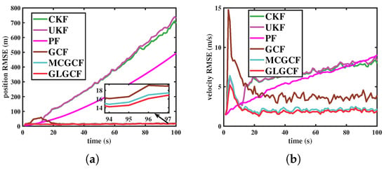
Figure 1. RMSEs of different filters in estimating the CV model under the scenario 1. (a) Position (m); (b) velocity (m/s).

4.1.2. Mixed Noise

Scenario 2: In this scenario, the measurement noise is assumed to follow an additive combination of two Gaussian noise distributions.

$$\begin{array}{cc}\hfill {\mathbf{v}}_k& \sim 0.5\mathcal{N}(\mathbf{0},0.1diag[{\left(20\mathrm{m}\right)}^2,{\left({\displaystyle \frac{2\pi }{180}}\mathrm{rad}\right)}^2])\hfill \\ \hfill & +0.5\mathcal{N}(\mathbf{0},0.1diag[{\left(30\mathrm{m}\right)}^2,{\left({\displaystyle \frac{4\pi }{180}}\mathrm{rad}\right)}^2]),\hfill \end{array}$$

(51)

The initial state is generated from ${\mathbf{x}}_0\sim \mathcal{N}\left({\widehat{\mathbf{x}}}_0,{\mathbf{P}}_0\right)$, where $\mathcal{N}({\widehat{\mathbf{x}}}_0,{\mathbf{P}}_0)$ is a Gaussian distribution with mean ${\widehat{\mathbf{x}}}_0={\left[100\mathrm{m},30\mathrm{m}/\mathrm{s},100\mathrm{m},20\mathrm{m}/\mathrm{s}\right]}^{\mathrm{T}}$ and with covariance ${\mathbf{P}}_0=diag{\left[10{\mathrm{m}}^2,1{\mathrm{m}}^2/{\mathrm{s}}^2,10{\mathrm{m}}^2,1{\mathrm{m}}^2/{\mathrm{s}}^2\right]}^{\mathrm{T}}$. The sampling period T = 1 s. The process noise covariance is ${\mathbf{Q}}_k^w=diag[0.01M,0.01M]$ with $M=\left[T^3/4,T^3/2;T^2/2,T\right]$. For GLGCF, the parameters t and c are set as 10 and 1, respectively. The minimum shape parameter is set as ${\mu }_{min}=-15$. The results of state estimate are obtained after 50 Monte Carlo runs.

The comparative results of different filters in the presence of mixed measurement noise are shown in Figure 2, Table 2 and Table 3. In comparison to the UKF, CKF, GCF, and PF, both the MCGCF and the GLGCF exhibit better performance. This is due to the use of the generalized transformation, which limits the higher-order errors associated with the DS technique, resulting in improved accuracy. Futhermore, as can be seen in Figure 2, Table 2 and Table 3, the proposed GLGCF algorithm achieves the highest estimation accuracy, demonstrating its superior performance in predicting both position and velocity estimation in the mixed-noise environment.

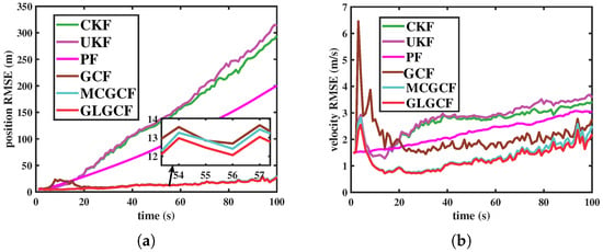
Figure 2. RMSEs of different filters in estimating the CV model under the scenario 2. (a) Position (m); (b) velocity (m/s).

Table 2. ARMSE of position (m) in the CV model under the different scenarios.

Scenarios	UKF	CKF	PF	GCF	MCGCF	GLGCF
Scenario 1	331.0570	321.7577	200.8265	19.9223	14.0247	13.6668
Scenario 2	139.9913	132.5550	89.1356	14.9162	13.1251	12.6863

Table 3. ARMSE of velocity (m/s) in the CV model under the different scenarios.

Scenarios	UKF	CKF	PF	GCF	MCGCF	GLGCF
Scenario 1	6.5610	6.4221	5.6947	4.2621	2.2781	2.0044
Scenario 2	2.7687	2.6409	2.2559	2.0620	1.3540	1.2733

4.2. Cooperative Turning Tracking Model

In this simulation, the cooperative turning (CT) target-tracking model is used to evaluate the filtering performance of the proposed GLGCF algorithm under heavy-tailed and mixed-noise environments. The CT model is well known as a fundamental maneuvering model in surface target tracking and is especially prevalent in describing the dynamics of maneuvering targets in unmanned surface vehicle tracking. The state and measurement equations for the CT model are presented below:

$$\begin{array}{cc}\hfill {\mathbf{x}}_k& =\left[\begin{array}{cccc}1& {\displaystyle \frac{sin\mathsf{\Omega }T}{\mathsf{\Omega }}}& 0& -\left({\displaystyle \frac{1-cos\mathsf{\Omega }T}{\mathsf{\Omega }}}\right)\\ 0& cos\mathsf{\Omega }T& 0& -sin\mathsf{\Omega }T\\ 0& {\displaystyle \frac{1-cos\mathsf{\Omega }T}{\mathsf{\Omega }}}& 1& {\displaystyle \frac{sin\mathsf{\Omega }T}{\mathsf{\Omega }}}\\ 0& sin\mathsf{\Omega }T& 0& cos\mathsf{\Omega }T\end{array}\right]{\mathbf{x}}_{k-1}+{\mathbf{w}}_k,\hfill \end{array}$$

(52)

$$\begin{array}{cc}\hfill {\mathbf{z}}_k& =\left[\begin{array}{c}\sqrt{{\alpha }_k^2+{\beta }_k^2}\hfill \\ arctan{\displaystyle \frac{{\beta }_k}{{\alpha }_k}}\hfill \end{array}\right]+{\mathbf{v}}_k,\hfill \end{array}$$

(53)

where ${\mathbf{x}}_k\triangleq {\left[{\alpha }_k,{\dot{\alpha }}_k,{\beta }_k,{\dot{\beta }}_k\right]}^{\mathrm{T}}$ with position $({\alpha }_k,{\dot{\alpha }}_k)$ and velocity $({\beta }_k,{\dot{\beta }}_k).$T represents the sampling period, and $\mathsf{\Omega }$ represents the tuning rate. ${\mathbf{w}}_k$ denotes the process noise with its covariance matrix ${\mathbf{Q}}_k^w$, and ${\mathbf{v}}_k$ represents the measurement noise with covariance matrix ${\mathbf{R}}_k^v$.

We consider the four scenarios with different measurement noise models below.

4.2.1. Heavy-Tailed Noise

Scenario 1: The robustness of the GLGCF algorithm against non-Gaussian noise is demonstrated by assuming the measurement noise in Equation (53) to be heavy-tailed, generated by a mixture of Gaussian distributions with different variances:

$$\begin{array}{cc}\hfill {\mathbf{v}}_k& \sim 0.9\mathcal{N}(\mathbf{0},\mathrm{diag}[{\left(10\mathrm{m}\right)}^2,{\left(\sqrt{10}\mathrm{mrad}\right)}^2])\hfill \\ \hfill & +0.1\mathcal{N}(\mathbf{0},400\mathrm{diag}[{\left(10\mathrm{m}\right)}^2,{\left(\sqrt{10}\mathrm{mrad}\right)}^2]),\hfill \end{array}$$

(54)

Scenario 2: The probability of large outliers in the measurement noise is increased as follows:

$$\begin{array}{cc}\hfill {\mathbf{v}}_k& \sim 0.8\mathcal{N}(\mathbf{0},\mathrm{diag}[{\left(10\mathrm{m}\right)}^2,{\left(\sqrt{10}\mathrm{mrad}\right)}^2])\hfill \\ \hfill & +0.2\mathcal{N}(\mathbf{0},400\mathrm{diag}[{\left(10\mathrm{m}\right)}^2,{\left(\sqrt{10}\mathrm{mrad}\right)}^2]).\hfill \end{array}$$

(55)

The initial state is generated from ${\mathbf{x}}_0\sim \mathcal{N}\left({\widehat{\mathbf{x}}}_0,{\mathbf{P}}_0\right)$, where $\mathcal{N}({\widehat{\mathbf{x}}}_0,{\mathbf{P}}_0)$ is a Gaussian distribution with mean ${\widehat{\mathbf{x}}}_0={\left[100\mathrm{m},80\mathrm{m}/\mathrm{s},100\mathrm{m},120\mathrm{m}/\mathrm{s}\right]}^{\mathrm{T}}$ and with covariance ${\mathbf{P}}_0=\mathrm{diag}{\left[10{\mathrm{m}}^2,1{\mathrm{m}}^2/{\mathrm{s}}^2,10{\mathrm{m}}^2,1{\mathrm{m}}^2/{\mathrm{s}}^2\right]}^{\mathrm{T}}$. The sampling period T = 1 s and tuning rate $\mathsf{\Omega }={\displaystyle \frac{\pi }{19}}$ rad. The process noise covariance is ${\mathbf{Q}}_k^w=\mathrm{diag}[0.04M,0.04M]$ with $M=\left[T^3/3,T^3/2;T^2/2,T\right]$. For GLGCF, the parameters t and c are set as 10 and 1, respectively. The minimum shape parameter is set as ${\mu }_{min}=-15$. The results of the state estimate are obtained after 50 Monte Carlo runs.

The RMSEs for different algorithms under heavy-tailed noise in scenario 1 and scenario 2 are depicted in Figure 3 and Figure 4, respectively. The ARMSEs of position and velocity estimates in scenarios 1 and 2 are summarized in Table 4 and Table 5, respectively. As shown in Figure 3 and Figure 4, the filtering accuracy of GLGCF is superior to GCF, MCGCF, CKF, and UKF. This confirms that incorporating the GL into the GCF improves the estimation accuracy and robustness of the filter when dealing with heavy-tailed noise. In the presence of measurement noise that includes outliers, the GCF suffers from performance degradation. However, the use of MCC and GL function stabilizes the GCF by performing nonlinear iterations on the anomalous measurements. Both MCGCF and GLGCF maintain stable performance, with GLGCF achieving superior performance. The results indicate that, in the non-Gaussian noise environments, the optimal form of the loss function can be automatically determined by the error distribution, thanks to the use of the residual optimization parameter.

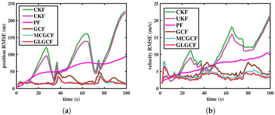
Figure 3. RMSEs of different filters in estimating the CT model under the scenario 1. (a) Position (m); (b) velocity (m/s).

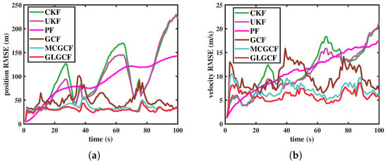
Figure 4. RMSEs of different filters in estimating the CT model under the scenario 2. (a) Position (m); (b) velocity (m/s).

Table 4. ARMSE of position (m) in the CT model under the different scenarios.

Scenarios	UKF	CKF	PF	GCF	MCGCF	GLGCF
Scenario 1	85.2765	94.7279	58.2086	23.2924	17.1634	16.2886
Scenario 2	94.5022	101.3773	89.3779	49.4746	34.2448	30.4771
Scenario 3	23.8895	25.5105	23.0006	12.8505	11.1167	9.1751
Scenario 4	23.7951	23.0617	21.2383	12.9255	8.2138	7.8886

Table 5. ARMSE of velocity (m/s) in the CT model under the different scenarios.

Scenarios	UKF	CKF	PF	GCF	MCGCF	GLGCF
Scenario 1	9.3098	10.2566	6.6212	4.8973	4.0205	3.5092
Scenario 2	10.7348	11.3610	11.1311	9.5834	6.9961	5.9547
Scenario 3	3.0411	3.2034	2.5192	1.8945	1.5966	1.3459
Scenario 4	2.9521	2.9545	2.4829	1.9109	1.3261	1.2425

4.2.2. Mixed Noise

Scenario 3: The measurement noise is characterized by a mixture of Gaussian distributions, with different variances for the position and velocity:

$$\begin{array}{cc}\hfill {\mathbf{v}}_k& \sim 0.5\mathcal{N}(\mathbf{0},0.05\mathrm{diag}[{\left(25\mathrm{m}\right)}^2,{\left({\displaystyle \frac{3\pi }{180}}\mathrm{rad}\right)}^2])\hfill \\ \hfill & +0.5\mathcal{N}(\mathbf{0},0.05\mathrm{diag}[{\left(30\mathrm{m}\right)}^2,{\left({\displaystyle \frac{9\pi }{180}}\mathrm{rad}\right)}^2]),\hfill \end{array}$$

(56)

Scenario 4: In this scenario, the measurement noise is also a mixture of two Gaussian distributions, with the following mixture weights:

$$\begin{array}{cc}\hfill {\mathbf{v}}_k& \sim 0.7\mathcal{N}(\mathbf{0},0.05\mathrm{diag}[{\left(25\mathrm{m}\right)}^2,{\left({\displaystyle \frac{3\pi }{180}}\mathrm{rad}\right)}^2])\hfill \\ \hfill & +0.3\mathcal{N}(\mathbf{0},0.05\mathrm{diag}[{\left(30\mathrm{m}\right)}^2,{\left({\displaystyle \frac{9\pi }{180}}\mathrm{rad}\right)}^2]).\hfill \end{array}$$

(57)

The initial state is generated from ${\mathbf{x}}_0\sim \mathcal{N}\left({\widehat{\mathbf{x}}}_0,{\mathbf{P}}_0\right)$, where $\mathcal{N}({\widehat{\mathbf{x}}}_0,{\mathbf{P}}_0)$ is a Gaussian distribution with mean ${\widehat{\mathbf{x}}}_0={\left[100\mathrm{m},80\mathrm{m}/\mathrm{s},100\mathrm{m},120\mathrm{m}/\mathrm{s}\right]}^{\mathrm{T}}$ and with covariance ${\mathbf{P}}_0=\mathrm{text}{\left[10{\mathrm{m}}^2,1{\mathrm{m}}^2/{\mathrm{s}}^2,10{\mathrm{m}}^2,1{\mathrm{m}}^2/{\mathrm{s}}^2\right]}^{\mathrm{T}}$. The sampling period T = 1 s and tuning rate $\mathsf{\Omega }={\displaystyle \frac{\pi }{19}}$ rad. The process noise covariance is ${\mathbf{Q}}_k^w=\mathrm{diag}[0.04M,0.04M]$ with $M=\left[T^3/3,T^3/2;T^2/2,T\right]$. For GLGCF, the parameters t and c are set as 10 and 1, respectively. The minimum shape parameter is set as ${\mu }_{min}=-15$. The results of state estimate are obtained after 50 Monte Carlo runs.

Figure 5 and Figure 6 show the RMSE curves of UKF, CKF, GCF, MCGCF and GLGCF in the mixed measurement noise. Table 4 and Table 5 summarize the ARMSEs of position and velocity estimates in scenario 3 and scenario 4. It can be seen in Figure 5 and Figure 6, Table 4 and Table 5, the RMSE and ARMSE achieved by GLGCF algorithm are smaller than those of other compared algorithms. In the mixed-noise environment, the estimation accuracy of MCGCF and GLGCF becomes closer, with GLGCF still providing the best filtering accuracy. Compared to the heavy-tailed environment, the advantage of GLGCF is less distinct in the mixed-noise environment. This can be attributed to the absence of large outliers in the measurement noise, where both GCF and MCGCF offer good filtering results. Therefore, GLGCF exhibits its robustness against the impact of outliers, providing superior performance in more complex environments.

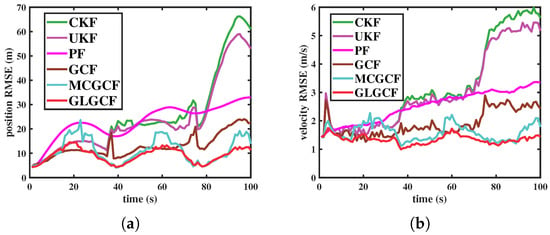
Figure 5. RMSEs of different filters in estimating the CT model under the scenario 3. (a) Position (m); (b) velocity (m/s).

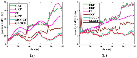
Figure 6. RMSEs of different filters in estimating the CT model under the scenario 4. (a) Position (m); (b) velocity (m/s).

5. Conclusions

In this paper, an extended version of the generalized conversion filter (GCF), namely generalized loss-based generalized conversion filter (GLGCF), is proposed. The GCF performs well in the Gaussian noise environment. However, the performance of GCF is significantly deteriorated when the system encounters non-Gaussian noise, primarily due to the the characteristics of the minimum mean square error (MMSE) criterion. To tackle this challenge, the proposed GLGCF algorithm is reformulated using a nonlinear regression model, employing the generalized loss (GL) instead of MMSE criterion to estimate the system state. Moreover, the residual vectors are incorporated into the negative log-likelihood of GL to optimize the parameters, thereby reducing the burden for manual tuning. Finally, two simulations on target-tracking models are carried out to verify the effectiveness and robustness of the proposed GLGCF algorithm. The results indicate that this proposed GLGCF algorithm exhibits excellent performance when the system is affected by non-Gaussian noise.

References

- Xia, X.; Xiong, L.; Huang, Y.; Liu, Y.; Gao, L.; Xu, N.; Yu, Z. Estimation on IMU yaw misalignment by fusing information of automotive onboard sensors. Mech. Syst. Signal Process. 2022, 162, 107993. [Google Scholar] [CrossRef]
- Duník, J.; Biswas, S.K.; Dempster, A.G.; Pany, T.; Closas, P. State estimation methods in navigation: Overview and application. IEEE Aerosp. Electron. Syst. Mag. 2020, 35, 16–31. [Google Scholar] [CrossRef]
- Kalman, R.E. A new approach to linear filtering and prediction problems. Trans. ASME, Ser. D J. Basic Eng. 1960, 82, 35–45. [Google Scholar] [CrossRef]
- Ding, L.; Wen, C. High-Order extended Kalman filter for state estimation of nonlinear systems. Symmetry 2024, 16, 617. [Google Scholar] [CrossRef]
- Garcia, R.V.; Pardal, P.C.P.M.; Kuga, H.K.; Zanardi, M.C. Nonlinear filtering for sequential spacecraft attitude estimation with real data: Cubature Kalman Filter, Unscented Kalman Filter and Extended Kalman Filter. Adv. Space Res. 2019, 63, 1038–1050. [Google Scholar] [CrossRef]
- Wan, J.; Ren, P.; Guo, Q. Application of interactive multiple model adaptive five-degree cubature Kalman algorithm based on fuzzy logic in target tracking. Symmetry 2019, 11, 767. [Google Scholar] [CrossRef]
- Klokov, A.; Kanouj, M.; Mironchev, A. A novel carrier tracking approach for GPS signals based on gauss–hermite Kalman filter. Electronics 2022, 11, 2215. [Google Scholar] [CrossRef]
- Julier, S.J.; Uhlmann, J.K. Unscented filtering and nonlinear estimation. Proc. IEEE 2004, 92, 401–422. [Google Scholar] [CrossRef]
- Jouin, M.; Gouriveau, R.; Hissel, D.; Péra, M.C.; Zerhouni, N. Particle filter-based prognostics: Review, discussion and perspectives. Mech. Syst. Signal Process. 2016, 72–73, 2–31. [Google Scholar] [CrossRef]
- Liu, Y.; Li, X.R.; Chen, H. Linear estimation with transformed measurement for nonlinear estimation. IEEE Trans. Aerosp. Electron. Syst. 2016, 52, 221–236. [Google Scholar] [CrossRef]
- Lan, J.; Li, X.R. Nonlinear estimation by LMMSE-based estimation with optimized uncorrelated augmentation. IEEE Trans. Signal Process. 2015, 63, 4270–4283. [Google Scholar] [CrossRef]
- Lan, J.; Li, X.R. Nonlinear estimation based on conversion-sample optimization. Automatica 2020, 121, 109160. [Google Scholar] [CrossRef]
- Lan, J. Generalized-conversion-based nonlinear filtering using deterministic sampling for target tracking. IEEE Trans. Aerosp. Electron. Syst. 2023, 59, 7295–7307. [Google Scholar] [CrossRef]
- Schick, I.C.; Mitter, S.K. Robust recursive estimation in the presence of heavy-tailed observation noise. Ann. Statist. 1994, 22, 1045–1080. [Google Scholar] [CrossRef]
- Wang, S.; Wang, Z.; Dong, H.; Chen, Y.; Alsaadi, F.E. Recursive quadratic filtering for linear discrete non-Gaussian systems over time-correlated fading channels. IEEE Trans. Signal Process. 2022, 70, 3343–3356. [Google Scholar] [CrossRef]
- Battilotti, S.; Cacace, F.; d’Angelo, M.; Germani, A. The polynomial approach to the LQ non-Gaussian regulator problem through output injection. IEEE Trans. Autom. Control 2019, 64, 538–552. [Google Scholar] [CrossRef]
- Huang, Y.; Zhang, Y.; Xu, B.; Wu, Z.; Chambers, J. A new outlier-robust student’s t based gaussian approximate filter for cooperative localization. IEEE/ASME Trans. Mechatronics 2017, 22, 2380–2386. [Google Scholar] [CrossRef]
- Chen, B.; Dang, L.; Zheng, N.; Príncipe, J.C. Kalman Filtering Under Information Theoretic Criteria; Springer: Cham, Switzerland, 2023. [Google Scholar]
- Chen, B.; Liu, X.; Zhao, H.; Príncipe, J.C. Maximum correntropy Kalman filter. Automatica 2017, 76, 70–77. [Google Scholar] [CrossRef]
- Dang, L.; Jin, S.; Ma, W.; Chen, B. Maximum correntropy generalized conversion-based nonlinear filtering. IEEE Sens. J. 2024, 24, 37300–37310. [Google Scholar] [CrossRef]
- Chen, B.; Dang, L.; Gu, Y.; Zheng, N.; Príncipe, J.C. Minimum errorentropy Kalman filter. IEEE Trans. Syst. Man Cybern. Syst. 2019, 51, 5819–5829. [Google Scholar] [CrossRef]
- Barron, J.T. A general and adaptive robust loss function. In Proceedings of the IEEE/CVF Conference on Computer Vision and Pattern Recognition (CVPR), Long Beach, CA, USA, 15–20 June 2019; pp. 4331–4339. [Google Scholar]
- Charbonnier, P.; Blanc-Feraud, L.; Aubert, G.; Barlaud, M. Two deterministic half-quadratic regularization algorithms for computed imaging. In Proceedings of the 1st International Conference on Image Processing, Austin, TX, USA, 13–16 November 1994; Volume 2, pp. 168–172. [Google Scholar]
- Qi, L.; Shen, M.; Wang, D.; Wang, S. Robust cauchy kernel conjugate gradient algorithm for non-Gaussian noises. IEEE Signal Process. Lett. 2021, 28, 1011–1015. [Google Scholar] [CrossRef]
- Lu, L.; Wang, W.; Yang, X.; Wu, W.; Zhu, G. Recursive GemanMcClure estimator for implementing second-order Volterra filter. IEEE Trans. Circuits Syst. II Exp. Briefs. 2019, 66, 1272–1276. [Google Scholar]
- Dennis, J.E.; Welsch, R.E. Techniques for nonlinear least squares and robust regression. Commun. Statist.-Simul. Comput. 1978, 7, 345–359. [Google Scholar] [CrossRef]
- Yan, W.; Chen, S.; Lin, D.; Wang, S. Variational Bayesian-based generalized loss cubature Kalman Filter. IEEE Trans. Circuits Syst. II Express Briefs. 2024, 71, 2874–2878. [Google Scholar] [CrossRef]
- Zhao, H.; Hu, J. Iterative unscented Kalman filter with general robust loss function for power system forecasting-aided state estimation. IEEE Trans. Instrum. Meas. 2023, 73, 9503809. [Google Scholar] [CrossRef]
- Chen, S.; Zhang, Q.; Lin, D.; Wang, S. Generalized loss based geometric unscented Kalman filter for robust power system forecasting-aided state estimation. IEEE Signal Process Lett. 2022, 29, 2353–2357. [Google Scholar] [CrossRef]
- Liu, W.; Pokharel, P.P.; Principe, J.C. Correntropy: Properties, and applications in non-Gaussian signal processing. IEEE Trans. Signal Process. 2007, 55, 5286–5298. [Google Scholar] [CrossRef]
- Zhu, B.; Chang, L.; Xu, J.; Zha, F.; Li, J. Huber-based adaptive unscented Kalman filter with non-Gaussian measurement noise. Circuits, Syst. Signal Process. 2018, 37, 3842–3861. [Google Scholar] [CrossRef]
- Chebrolu, N.; Labe, T.; Vysotska, O.; Behley, J.; Stachniss, C. Adaptive robust kernels for non-linear least squares problems. IEEE Robot. Autom. Lett. 2021, 6, 2240–2247. [Google Scholar] [CrossRef]
- Arasaratnam, I.; Haykin, S. Cubature Kalman filters. IEEE Trans. Autom. Control. 2009, 54, 1254–1269. [Google Scholar] [CrossRef]
- Arulampalam, M.S.; Maskell, S.; Gordon, N.; Clapp, T. A tutorial on particle filters for online nonlinear/non-Gaussian Bayesian tracking. IEEE Trans. Signal Process. 2002, 50, 174–188. [Google Scholar] [CrossRef]
Disclaimer/Publisher’s Note: The statements, opinions and data contained in all publications are solely those of the individual author(s) and contributor(s) and not of MDPI and/or the editor(s). MDPI and/or the editor(s) disclaim responsibility for any injury to people or property resulting from any ideas, methods, instructions or products referred to in the content. |
© 2025 by the authors. Licensee MDPI, Basel, Switzerland. This article is an open access article distributed under the terms and conditions of the Creative Commons Attribution (CC BY) license (https://creativecommons.org/licenses/by/4.0/).