On the Distribution of the Random Sum and Linear Combination of Independent Exponentiated Exponential Random Variables

Abstract

The exponentiated exponential distribution has received great attention from many statisticians due to its popularity, many applications, and the fact that it is an efficient alternative to many famous distributions such as Weibull and gamma distributions. Many statisticians have studied the mathematical properties of this distribution and estimated its parameters under different censoring schemes. However, it seems that the distribution of the random sum, the distribution of the linear combination, and the value of the reliability index, $R=P(X_2<X_1)$, in the case of unequal scale parameters, were not known for this distribution. Therefore, in this article, we present the saddlepoint approximation to the distribution of the random sum, the distribution of linear combination, and the value of the reliability index $R=P(X_2<X_1)$ for exponentiated exponential variates. These saddlepoint approximations are computationally appealing, and numerical studies confirm their accuracy. In addition to the accuracy provided by the saddlepoint approximation method, it saves time compared to the simulation method, which requires a lot of time. Therefore, the saddlepoint approximation method provides an outstanding balance between precision and computational efficiency.

1. Introduction

The exponentiated exponential (EE) distribution was introduced by Gupta and Kundu [1]. It has become a prominent generalization of the classical exponential distribution. Its flexibility and asymmetrical structure enable more precise modeling of various real-world phenomena characterized by non-monotonic hazard functions, making it a valuable tool in many areas, such as reliability analysis, survival analysis, and actuarial science. The primary advantage of the EE distribution is its ability to model more complex lifetime behaviors compared to the standard exponential distribution, which assumes a constant hazard rate. In contrast, the EE distribution offers more shape flexibility, accommodating increasing and decreasing hazard rates. This makes it particularly useful for systems where the risk of failure or event occurrence varies over time, such as in biomedical research, engineering reliability, and ecological studies. Another significant benefit is that the EE distribution provides closed-form expressions for important characteristics like the cumulative distribution function (CDF), moments, moment-generating function (MGF), and reliability measures. This mathematical simplicity enhances its computational efficiency, making it suitable for both theoretical analysis and practical applications. Many authors have studied the EE distribution, among them: Gupta and Kundu [2,3], Zheng [4], Sarhan [5], Abdel-Hamid and Al-Hussaini [6], Chen and Lio [7], Ismail [8], Han and Kundu [9], Ateya and Mohammed [10], Pandey et al. [11], and Kabdwal et al. [12].

A random variable X is defined to follow the EE distribution if its probability density function (PDF) and CDF are expressed as:

$$g\left(x\right)=\alpha \beta \exp (-\beta x){\left(1-\exp (-\beta x)\right)}^{\alpha -1},x>0,\alpha >0\mathrm{and}\beta >0,$$

(1)

and

$$G\left(x\right)={\left(1-\exp (-\beta x)\right)}^{\alpha }.$$

(2)

This paper addresses unexplored aspects of the exponentiated exponential distribution, specifically, the distributions of the random sum, the linear combination of independent exponentiated exponential random variables, and the reliability index $R=P(X_2<X_1)$, particularly in cases with unequal scale parameters. It introduces and applies the saddlepoint approximation method to calculate these distributions and the reliability index. This is novel, as previous works have not focused on these aspects of the exponentiated exponential distribution. The saddlepoint approximation is highlighted as a computationally efficient alternative to exact simulation methods, offering the advantage of maintaining high accuracy while significantly reducing computation time. The key contributions of this study include bridging theoretical gaps in the exponentiated exponential (EE) distribution by deriving saddlepoint approximations for previously unexplored properties. The work demonstrates an effective balance between computational efficiency and precision, making it particularly valuable for applications that require rapid and accurate reliability assessments. Additionally, it provides a foundation for extending saddlepoint methods to more complex scenarios, such as bivariate distributions, paving the way for future research.

A random sum, or stopped sum, refers to the total obtained by summing a random number of random variables. This concept is widely applicable in many fields such as actuarial science, queuing theory, reliability engineering, and finance, where sums of random variables often come with a stopping rule defined by an independent random variable. Mathematically, let N be a discrete random variable indicating the stopping point, and let $X_1,X_2,\cdots ,X_N$ be independent and identically distributed random variables; then, the random sum is given by $S_N=X_1+X_2+\cdots +X_N$. It can effectively model a variety of real-world phenomena [13]. In actuarial science, random sums are used to model the total claim amount for insurance portfolios, where the number of claims is distributed (often as Poisson or Negative Binomial), and each claim amount represents a random variable. In queuing systems, random sums help evaluate total waiting times and service durations, offering insights for resource allocation and customer service optimization. In reliability engineering, random sums model the lifetime of a system that fails once a certain number of component failures occur, facilitating maintenance planning and replacement scheduling. In finance, random sums can represent cumulative returns on assets in a portfolio with investments made at random intervals, supporting risk management and strategic investment planning. For more applications of the random sum, see Rao et al. [14] and Malinovskii [15].

The distribution of a linear combination of n random variables is fundamental in statistics and probability theory. The linear combination is expressed as $L_n=k_1{X}_1+k_2{X}_2+\dots +k_n{X}_n,$, where $X_i$ represents random variables, and $k_i$ are constants. This concept finds extensive applications across various fields, including finance, where portfolio returns are modeled as a linear combination of returns from individual assets [16]. In hydrology, the net flow from a reservoir basin is determined by subtracting the amount of water used for purposes such as domestic consumption and agriculture from the total rainfall in the area [17]. For more applications of the distribution of the linear combination of random variables, see Arellano and Gento [18], Nadarajah [17], Marques et al. [19], and Krishnamoorthy [20].

In the context of reliability, the stress–strength model illustrates the lifespan of a component characterized by a random strength $X_1$ and subjected to random stress $X_2$. The component fails when the applied stress exceeds its strength while it continues to operate effectively whenever $X_1>X_2$. Consequently, the reliability index $R=P(X_2<X_1)$ indicates the likelihood of the component operating without failure. This model finds extensive applications in various engineering domains, including structural integrity assessments, the deterioration of rocket motors, static fatigue in ceramic materials, fatigue failures in aircraft structures, and the aging of concrete pressure vessels. For more details, see Weerahandi and Johnson [21], Kohansal [22], Kayal et al. [23], and Pakdaman et al. [24].

The saddlepoint approximation was first introduced to statistics by Daniels [25]. This approximation method provides an approach to approximate a density or mass function using its moment-generating or cumulant-generating function. Lugannani and Rice [26] later proposed a saddlepoint approximation to the CDF of continuous distributions. Daniels [27] introduced two continuity modifications for discrete distributions. Barndorff-Nielsen and Cox [28] developed a saddlepoint density approximation for conditional distributions, and Skovgaard [29] extended this with a double saddlepoint approximation for the CDF. The saddlepoint approximation is widely recognized for its exceptional accuracy in statistical computations, especially in approximating distributions that are challenging to derive precisely. This method achieves a high level of precision in approximating probabilities and reliability indices, often producing results that closely align with those obtained through exact methods. The saddlepoint approximation method stands out among asymptotic approximation methods due to its superior accuracy and robustness. While many asymptotic methods rely on large-sample assumptions that can lead to significant errors in small or moderate samples, the saddlepoint approximation delivers precise results even in these scenarios. It effectively captures the behavior of the distribution’s tail and central regions, where other asymptotic methods may struggle. For a comprehensive review and applications of saddlepoint approximations, refer to Butler [30]. For recent studies and advancements in saddlepoint approximation, see Alhejaili and Abd-Elfattah [31], Gatto [32], Abd El-Raheem and Abd-Elfattah [33,34], Meng et al. [35], Goodman [36], Abd El-Raheem et al. [37,38], Arevalillo [39], and Abd El-Raheem et al. [40,41].

This article discusses the saddlepoint approximations for the EE distribution in various contexts. Section 2 introduces the saddlepoint approximation to the Poisson-EE random sum distribution, accompanied by a simulation study (Section 2.1) and a numerical example (Section 2.2) to validate the results. Section 3 extends the analysis to a linear combination of EE random variables, presenting both a simulation study (Section 3.1) and a corresponding illustrative example (Section 3.2). Section 4 focuses on the saddlepoint approximation to the reliability index, $R=P(X_2<X_1)$, with a simulation study in Section 4.1 to evaluate its accuracy. Finally, Section 5 concludes the article by summarizing the findings and emphasizing the computational efficiency and accuracy of the proposed approximations.

2. Saddlepoint Approximation to the Poisson-EE Random Sum Distribution

In this section, the saddlepoint approximation to the Poisson-EE random sum distribution is derived. The Poisson-EE random sum is the sum of a random sample from the EE distribution with sample size, N, independent Poisson $\left(\lambda \right)$ random variables.

The saddlepoint approximation of the PDF, $g_X\left(x\right)$, is given by [25]:

$${\widehat{g}}_X\left(x\right)={\displaystyle \frac{1}{\sqrt{2\pi C_X^{″}\left(\widehat{t}\right)}}}\exp \left(C_X\left(\widehat{t}\right)-\widehat{t}x\right),$$

(3)

where $C_X\left(t\right)$ is the cumulant generating function (CGF) of X, $\widehat{t}=\widehat{t}\left(x\right)$ is the unique solution to the saddlepoint equation

$$C_X^{\prime }\left(\widehat{t}\right)={\displaystyle \frac{\partial C_X\left(t\right)}{\partial t}}=x,$$

The saddlepoint approximation of the CDF, $G_X\left(x\right)$, is given by [26]:

$${\widehat{G}}_X\left(x\right)=\left\{\begin{array}{cc}\mathsf{\Psi }\left(\widehat{u}\right)+\psi \left(\widehat{u}\right)\left({\displaystyle \frac{1}{\widehat{u}}}-{\displaystyle \frac{1}{\widehat{v}}}\right),\hfill & \mathrm{if}x\ne \mu \hfill \\ {\displaystyle \frac{1}{2}}+{\displaystyle \frac{C_X^{\prime \prime \prime }\left(0\right)}{6\sqrt{2\pi C_X^{\prime \prime }{\left(0\right)}^3}}},\hfill & \mathrm{if}x=\mu ,\hfill \end{array}\right.$$

(4)

where $\mathsf{\Psi }$ and $\psi$ represent the CDF and PDF of the standard normal distribution, respectively, and $\mu$ is the mean of the distribution. Here, $\widehat{u}=\mathrm{sgn}\left(\widehat{t}\right)\sqrt{2(\widehat{t}x-C_X\left(\widehat{t}\right))}$ and $\widehat{v}=\widehat{t}\sqrt{C^{″}\left(\widehat{t}\right)}$.

Let $M_N\left(t\right)$ and $M_X\left(t\right)$ be the MGFs of N and X, respectively. It is easy to show that the MGF of $S_N$ is given by:

$$M_{S_N}\left(t\right)=M_N(log{M}_X\left(t\right)),$$

and its CGF is given by:

$$C_{S_N}\left(t\right)=C_N\left(C_X\left(t\right)\right),$$

where $C_N\left(t\right)=log{M}_N\left(t\right)$ and $C_X\left(t\right)=log{M}_X\left(t\right)$ are the CGFs of N and X, respectively.

By replacing $C_X\left(t\right)$ with $C_{S_N}\left(t\right)$ in (3), the saddlepoint approximation to the PDF of $S_N$ is given by:

$${\widehat{g}}_{S_N}\left(s\right)=\exp \left(C_N\left(C_X\left(\widehat{t}\right)\right)-\widehat{t}s\right){\left(2\pi \left(C_N^{\prime \prime }\left(C_X\left(\widehat{t}\right)\right)C_X^{\prime }{\left(\widehat{t}\right)}^2+C_X^{\prime \prime }\left(\widehat{t}\right)C_N^{\prime }\left(C_X\left(\widehat{t}\right)\right)\right)\right)}^{-{\displaystyle \frac{1}{2}}}.$$

(5)

The saddlepoint approximation to the CDF of $S_N$ is given by:

$${\widehat{G}}_{S_N}\left(s\right)=\left\{\begin{array}{cc}\mathsf{\Psi }\left(\widehat{u}\right)+\psi \left(\widehat{u}\right)\left({\displaystyle \frac{1}{\widehat{u}}}-{\displaystyle \frac{1}{\widehat{v}}}\right),\hfill & \mathrm{if}s\ne {\mu }_{S_N}\hfill \\ {\displaystyle \frac{1}{2}}+{\displaystyle \frac{C_{S_N}^{\prime \prime \prime }\left(0\right)}{6\sqrt{2\pi C_{S_N}^{\prime \prime }{\left(0\right)}^3}}},\hfill & \mathrm{if}s={\mu }_{S_N},\hfill \end{array}\right.$$

(6)

where

$$\widehat{u}=\mathrm{sgn}\left(\widehat{t}\right)\sqrt{2(\widehat{t}s-C_N\left(C_X\left(\widehat{t}\right)\right))},$$

and

$$\widehat{v}=\widehat{t}\sqrt{C_N^{″}\left(C_X\left(\widehat{t}\right)\right)C_X^{\prime }{\left(\widehat{t}\right)}^2+C_X^{″}\left(\widehat{t}\right)C_N^{\prime }\left(C_X\left(\widehat{t}\right)\right)},$$

with $\widehat{t}$ being the solution to the equation $C_N^{\prime }\left(C_X\left(\widehat{t}\right)\right)C_X^{\prime }\left(\widehat{t}\right)=s$, and $\mathrm{sgn}\left(\widehat{t}\right)$ representing the sign of $\widehat{t}$.

For the Poisson-EE random sum distribution, the CGF of $S_N$ is given by:

$$C_{S_N}\left(t\right)=C_N\left(C_X\left(t\right)\right)=\lambda \left({\displaystyle \frac{\mathsf{\Gamma }(\alpha +1)\mathsf{\Gamma }(1-\frac{t}{\beta })}{\mathsf{\Gamma }(\alpha -\frac{t}{\beta }+1)}}-1\right),\mathrm{for}0<t<\beta .$$

(7)

Thus, the saddlepoint equation is

$$C_{S_N}^{\prime }\left(\widehat{t}\right)={\displaystyle \frac{\lambda \mathsf{\Gamma }(\alpha +1)\mathsf{\Gamma }(\alpha -\frac{t}{\beta }+1)\mathsf{\Gamma }(1-\frac{t}{\beta })\left(-\phi (1-\frac{t}{\beta })+\phi (\alpha -\frac{t}{\beta }+1)\right)}{\beta {\left(\mathsf{\Gamma }(\alpha -\frac{t}{\beta }+1)\right)}^2}}=s,$$

(8)

where $\phi (.)$ is the digamma function. The saddlepoint $\widehat{t}$ can be obtained by solving Equation (8) numerically using the Newton–Raphson method.

The saddlepoint approximations to PDF and CDF of the Poisson-EE random sum distribution are given by (5) and (6), respectively.

2.1. Simulation Study

In this section, a simulation study is performed to evaluate the accuracy of the saddlepoint method for approximating the distribution of the Poisson-EE random sum. To verify the accuracy of the saddlepoint method, its results must be compared with the exact value, but the exact value cannot be calculated analytically, so we approximate the exact value using the simulation method in which we generate ${10}^6$ values of $S_N$, where each simulation involves generating a value N from a Poisson $\left(\lambda \right)$ distribution and then generating N values from the EE $(\alpha ,\beta )$ distribution. Thus, the simulated (exact) value of $G_{S_N}\left(s\right)$ can be obtained from the following formula:

$$G_{S_N}\left(s\right)=P(S_N\le s)={\displaystyle \frac{1}{{10}^6}}\sum _1^{{10}^6}I(S_N=X_1+X_2+\dots +X_N\le s),$$

(9)

where $I(.)$ is the indicator function.

During the article, we use the term “exact value” to refer to the value approximated using the simulation method.

The simulation study is carried out according to the following three scenarios of the parameters of the EE $(\alpha ,\beta )$ distribution:

• Scenario I: $\alpha =0.8$ and $\beta =0.5$.
• Scenario II: $\alpha =2.2$ and $\beta =1.2$.
• Scenario III: $\alpha =0.8$ and $\beta =1.4$.

The proposed scenarios allow for studying different shapes of the hazard rate function of the distribution under study. This diversity ensures that the accuracy of the saddlepoint approximation is tested across a diverse set of conditions.

The procedures for approximating the CDF of the Poisson-EE random sum distribution using the simulation and saddlepoint methods are carried out according to Algorithm 1.

Table 1 presents both the exact values and the saddlepoint approximations of $G_{S_N}\left(s\right)$ with the MSE of the saddlepoint approximation method for the different simulation scenarios. Moreover, the computing time in minutes for the simulation method (Time (exact)) and saddlepoint approximation method (Time (sadd)) are recorded and displayed in Table 1.

Algorithm 1: Approximating the CDF of the Poisson-EE random sum distribution.

Specify the values of the parameters $\lambda$, $\alpha$ and $\beta$. For the given value of the parameter $\lambda$, generate a random number N from the Poisson $\left(\lambda \right)$ distribution. For the given values of the parameters $\alpha$ and $\beta$, generate N random variables $X_i$, $i=1,2,\dots ,N$ from the EE $(\alpha ,\beta )$ distribution as follows: $$X_i=-{\displaystyle \frac{1}{\beta }}ln\left(1-U_i^{1/\alpha }\right),i=1,\cdots ,N,$$ where $U_i$ is a random variable from the uniform (0, 1) distribution. Evaluate the value of the random sum $S_N={\sum }_{i=1}^N{X}_i$. Use the saddlepoint approximation in (6) to approximate $G_{S_N}\left(s\right)=P(S_N\le s)$. Simulate ${10}^6$ values of $S_N$ under the same setup. Evaluate the simulated (exact) value of $G_{S_N}\left(s\right)=P(S_N\le s)$ using the simulated samples in step 6 and the formula in (9). Repeat steps 2 through 7 a thousand times. Evaluate the average of the values ${\widehat{G}}_{S_N}\left(s_l\right)$ and $G_{S_N}\left(s_l\right)$, $l=1,2,\dots ,1000$, where ${\widehat{G}}_{S_N}\left(s_l\right)$ and $G_{S_N}\left(s_l\right)$ are the approximated values of the CDF using the saddlepoint and simulation methods, respectively. Evaluate the mean square error (MSE) of the saddlepoint method compared to the exact value as $$MSE={\displaystyle \frac{1}{1000}}\sum _{l=1}^{1000}{\left(G_{S_N}\left(s_l\right)-{\widehat{G}}_{S_N}\left(s_l\right)\right)}^2.$$

Table 1. Exact and saddlepoint approximation of the CDF of the Poisson-EE random sum distribution.

Scenario	$\mathit{\lambda }$	${\overline{\mathit{S}}}_{\mathit{N}}$	${\mathit{G}}_{{\mathit{S}}_{\mathit{N}}}\left(\mathit{s}\right)$	${\widehat{\mathit{G}}}_{{\mathit{S}}_{\mathit{N}}}\left(\mathit{s}\right)$	MSE	Time (Exact)	Time (Sadd)
I	5	8.62021	0.49814	0.49775	1.393742 × 10${}^{-6}$	113.0680	0.01472
	8	13.96855	0.50518	0.50477	3.635884 × 10${}^{-7}$	115.0954	0.01354
	12	20.67394	0.49922	0.49903	2.117805 × 10${}^{-7}$	134.3281	0.01364
	16	27.25104	0.48363	0.48351	1.872718 × 10${}^{-7}$	150.5178	0.01394
	20	34.41974	0.49991	0.49982	1.640930 × 10${}^{-7}$	182.5806	0.01563
II	5	6.59247	0.49917	0.49919	9.409461 × 10${}^{-7}$	99.43792	0.01359
	8	10.61259	0.50601	0.50586	1.860925 × 10${}^{-7}$	110.6267	0.01332
	12	15.80302	0.50224	0.50218	1.700800 × 10${}^{-7}$	134.8183	0.01415
	16	20.73786	0.48276	0.48272	1.690641 × 10${}^{-7}$	134.8183	0.01415
	20	26.14338	0.49805	0.49803	1.533458 × 10${}^{-7}$	165.8390	0.01410
III	5	3.06960	0.49757	0.49718	1.394419 × 10${}^{-6}$	104.0224	0.01451
	8	4.98877	0.50518	0.50477	3.636125 × 10${}^{-7}$	116.5020	0.01542
	12	7.38355	0.49922	0.49903	2.117716 × 10${}^{-7}$	134.8595	0.01423
	16	9.73252	0.48363	0.48351	1.872615 × 10${}^{-7}$	149.5755	0.14348
	20	12.29276	0.49991	0.49982	1.640914 × 10${}^{-7}$	160.0325	0.01824

From the results in Table 1, we note the following key points:

• The saddlepoint approximation (${\widehat{G}}_{S_N}\left(s\right)$) closely matches the exact CDF ($G_{S_N}\left(s\right)$) with minimal MSEs across all scenarios and parameter settings.
• The differences between the two methods are negligible, typically on the order of ${10}^{-7}$ to ${10}^{-6}$, indicating high precision of the saddlepoint method.
• The simulation (exact) method requires significantly more computational time, ranging from approximately 99 to 182 min depending on the scenario and parameters. In contrast, the saddlepoint approximation is highly efficient, completing calculations in a fraction of a minute (approximately 0.013 to 0.018 min). This demonstrates the computational superiority of the saddlepoint method.
• In general, the saddlepoint approximation method provides an excellent balance between accuracy and computational efficiency, making it a convenient alternative to the simulation method for approximating the CDF of the Poisson-EE random sum distribution.

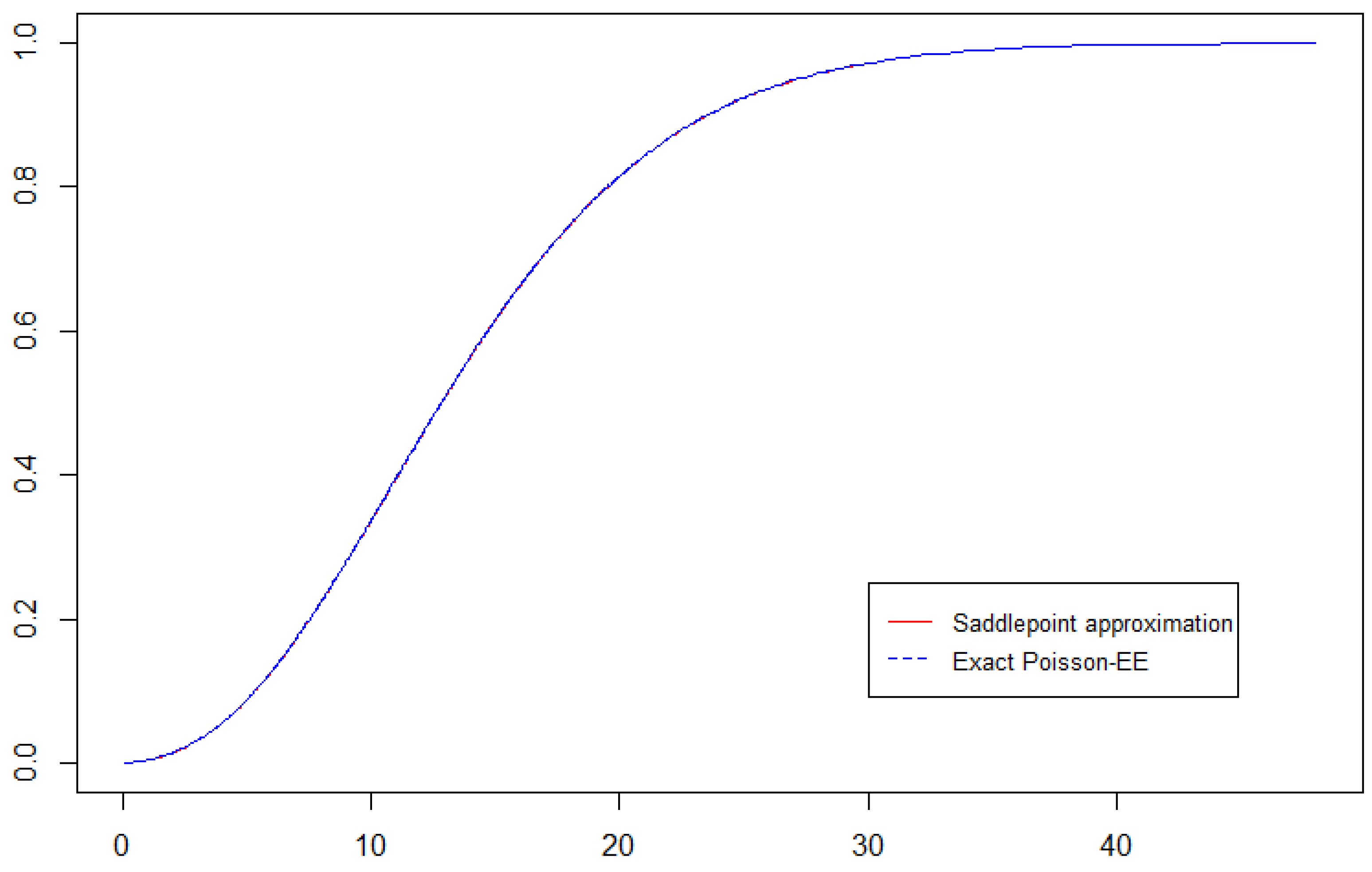
To demonstrate the accuracy of the saddlepoint approximation across a broad range of s values, a comparative plot of the exact CDF for the Poisson(8)-EE(0.8, 0.5) distribution alongside the saddlepoint approximation is presented in Figure 1.

Figure 1. The exact CDF for Poisson-EE random sum (blue dashed line) with its saddlepoint approximation (red solid line).

Figure 1 demonstrates the accuracy of the saddlepoint approximation in approximating the CDF of the Poisson-EE random sum over a broad range of values. The tight overlap between the two curves indicates that the saddlepoint method provides an excellent approximation.

2.2. Numerical Example

To demonstrate the proposed procedures in this section, we use a synthetic dataset representing the total healthcare costs for patients in a hospital. The total cost of care for a patient’s stay in a hospital may depend on a random number of procedures or treatments, each with a randomly distributed cost. The total cost is thus a random sum. Assume that the number of procedures or treatments, N, that the patient undergoes is a random variable following a Poisson $\left(\lambda \right)$ distribution and the cost of each treatment or medical procedure that the patient needs is a random variable, $X_i$, $i=1,2,\dots ,N$ following the EE $(\alpha ,\beta )$ distribution. Thus, we need to approximate the distribution of $S_N={\sum }_{i=1}^N{X}_i$. The following data, 44.81, 67.03, 45.91, 8.01, 24.52, 47.67, 38.42, represent the cost of a random number of medical services that a patient receives in a hospital, where the number of medical services is generated from the Poisson$\left(12\right)$ distribution and the cost of each service is generated from the EE $(4.2,0.05)$ distribution.

The saddlepoint approximation is used to approximate $G_{S_N}\left(s\right)=P({\sum }_{i=1}^N{X}_i<s)$ at different values of s. The results of the saddlepoint approximation ${\widehat{G}}_{S_N}\left(s\right)$ are presented in Table 2. The comparison between the second column ($G_{S_N}\left(s\right)$, the exact values) and the third column (${\widehat{G}}_{S_N}\left(s\right)$, the saddlepoint approximations) of Table 2 reveals that the two methods produce results that are extremely close to each other across all values of s. The discrepancies between the exact values and the approximations are generally negligible, often differing only in the third or fourth decimal place.

Table 2. Exact and saddlepoint approximation of $G_{S_N}\left(s\right)=P({\sum }_{i=1}^N{X}_i<s)$ for different values of s.

s	${\mathit{G}}_{{\mathit{S}}_{\mathit{N}}}\left(\mathit{s}\right)$	${\widehat{\mathit{G}}}_{{\mathit{S}}_{\mathit{N}}}\left(\mathit{s}\right)$
100	0.00116	0.00116
120	0.00226	0.00231
140	0.00430	0.00426
160	0.00737	0.00734
180	0.01197	0.01196
200	0.01856	0.01858
220	0.02756	0.02768
240	0.03964	0.03971
260	0.05510	0.05516
280	0.07409	0.07420
300	0.09717	0.09725
320	0.12416	0.12437
340	0.15522	0.15553
360	0.19036	0.19054
380	0.22904	0.22909
400	0.27056	0.27071
420	0.31474	0.31487
440	0.36116	0.36091
460	0.40820	0.40815
480	0.45598	0.45589
500	0.50336	0.50346
520	0.54999	0.55019
540	0.59541	0.59552
560	0.63881	0.63890
580	0.67956	0.68002
600	0.71821	0.71846
620	0.75383	0.75405
640	0.78657	0.78664
660	0.81589	0.81619
680	0.84259	0.84272
700	0.86604	0.86632
720	0.88681	0.88713
740	0.90500	0.90531
760	0.92076	0.92106
780	0.93448	0.93461
800	0.94581	0.94616

3. Saddlepoint Approximation to the Linear Combination of EE Random Variables

The linear combination of the EE random variables is given by:

$$L_n=k_1{X}_1+k_2{X}_2+\dots +k_n{X}_n,$$

(10)

where $X_1,X_2,\dots ,X_n$ are independent EE random variables, with shape parameter ${\alpha }_i>0$ and scale parameter ${\beta }_i>0$, and the $k_i$’s are real constants.

The MGFs of $X_i$ and $L_n={\sum }_{i=1}^n{k}_i{X}_i$ are respectively defined as:

$$M_{X_i}\left(\tau \right)={\displaystyle \frac{\mathsf{\Gamma }({\alpha }_i+1)\mathsf{\Gamma }(1-\frac{\tau }{{\beta }_i})}{\mathsf{\Gamma }({\alpha }_i-\frac{\tau }{{\beta }_i}+1)}},$$

(11)

and

$$M_{L_n}\left(\tau \right)=\prod _{i=1}^n{\displaystyle \frac{\mathsf{\Gamma }({\alpha }_i+1)\mathsf{\Gamma }(1-\frac{\tau k_i}{{\beta }_i})}{\mathsf{\Gamma }({\alpha }_i-\frac{\tau k_i}{{\beta }_i}+1)}}.$$

(12)

Thus, the CGF of $L_n={\sum }_{i=1}^n{k}_i{X}_i$ is given by:

$$C_{L_n}\left(\tau \right)=\sum _{i=1}^n\left(log\left(\mathsf{\Gamma }({\alpha }_i+1)\right)+log\left(\mathsf{\Gamma }(1-{\displaystyle \frac{\tau k_i}{{\beta }_i}})\right)-log\left(\mathsf{\Gamma }({\alpha }_i-{\displaystyle \frac{\tau k_i}{{\beta }_i}}+1)\right)\right),\mathrm{for}\tau k_i<{\beta }_i.$$

(13)

Let $g_{L_n}(\ell )$ be the PDF of $L_n$, then the saddlepoint approximation ${\widehat{g}}_{L_n}(\ell )$ is defined as:

$${\widehat{g}}_{L_n}(\ell )={\displaystyle \frac{1}{\sqrt{2\pi C_{L_n}^{\prime \prime }\left(\widehat{\tau }\right)}}}\exp \left(C_{L_n}\left(\widehat{\tau }\right)-\ell \widehat{\tau }\right),$$

(14)

where $\widehat{\tau }$ is the saddlepoint that satisfies th equation:

$$C_{L_n}^{\prime }\left(\widehat{\tau }\right)=\left(\phi \left(\alpha -{\displaystyle \frac{k_i\widehat{\tau }}{\beta }}+1\right)-\phi \left(1-{\displaystyle \frac{k_i\widehat{\tau }}{\beta }}\right)\right){\displaystyle \frac{k_i}{\beta }}=\ell ,\widehat{\tau }<\underset{i}{min}\left({\displaystyle \frac{{\beta }_i}{k_i}}\right).$$

(15)

The saddlepoint $\widehat{\tau }$ can be obtained by solving Equation (15) numerically using the Newton–Raphson method.

Let $G_{L_n}(\ell )$ be the CDF of $L_n$, then the saddlepoint approximation ${\widehat{G}}_{L_n}(\ell )$ is defined as

$${\widehat{G}}_{L_n}(\ell )=\left\{\begin{array}{cc}\mathsf{\Psi }\left({\widehat{\omega }}_1\right)+\psi \left({\widehat{\omega }}_1\right)\left({\displaystyle \frac{1}{{\widehat{\omega }}_1}}-{\displaystyle \frac{1}{{\widehat{\omega }}_2}}\right),\hfill & \mathrm{if}\ell \ne {\mu }_{L_n}\hfill \\ {\displaystyle \frac{1}{2}}+{\displaystyle \frac{C_{L_n}^{\prime \prime \prime }\left(0\right)}{6\sqrt{2\pi C_{L_n}^{\prime \prime }{\left(0\right)}^3}}},\hfill & \mathrm{if}\ell ={\mu }_{L_n},\hfill \end{array}\right.$$

(16)

where ${\widehat{\omega }}_1=\mathrm{sgn}\left(\widehat{\tau }\right)\sqrt{2(\widehat{\tau }\ell -C_{L_n}\left(\widehat{\tau }\right))}$ and ${\widehat{\omega }}_2=\widehat{\tau }\sqrt{C_{L_n}^{″}\left(\widehat{\tau }\right)}$.

The saddlepoint approximations to the PDF and CDF of the sum of n independent EE $({\alpha }_i,{\beta }_i)$ random variables, $S_n={\sum }_{i=1}^n{X}_i$, can be obtained as a special case of the saddlepoint approximations to the PDF and CDF of the linear combination, $L_n={\sum }_{i=1}^n{k}_i{X}_i$, when $k_i=1$.

3.1. Simulation Study

In this section, we conduct a simulation study to assess the accuracy of the saddlepoint method for approximating the distribution of the linear combination of n independent EE random variables, $L_n={\sum }_{i=1}^n{k}_i{X}_i$.

The simulation study is conducted according to the following scenarios of the parameters of the EE $({\alpha }_i,{\beta }_i)$ distribution and the constants $k_i$, $i=1,2,\dots ,n$.

• Scenario A: ${\alpha }_i=0.8$, ${\beta }_i=0.5$, and $k_i=2i+1$, $i=1,2,\dots ,n$.
• Scenario B: ${\alpha }_i=0.8$, ${\beta }_i=0.5$, and $k_i={(-1)}^{i+1}(i/3)$, $i=1,2,\dots ,n$.
• Scenario C: ${\alpha }_i=i/2$, ${\beta }_i=i/5$, and $k_i=2i+1$, $i=1,2,\dots ,n$.
• Scenario D: ${\alpha }_i=i/2$, ${\beta }_i=i/5$, and $k_i={(-1)}^{i+1}(i/3)$, $i=1,2,\dots ,n$.
• Scenario E: ${\alpha }_i=0.8$, ${\beta }_i=0.5$, and $k_i=1$, $i=1,2,\dots ,n$.
• Scenario F: ${\alpha }_i=i/2$, ${\beta }_i=i/5$, and $k_i=1$, $i=1,2,\dots ,n$.

Scenarios A, B, C, and D deal with the case of the linear combination, $L_n={\sum }_{i=1}^n{k}_i{X}_i$, while Scenarios E and F deal with the case of the sum, $S_n={\sum }_{i=1}^n{X}_i$. The parameter values ${\alpha }_i$ and ${\beta }_i$ are chosen to represent a diverse set of conditions, including both identically and non-identically random variable cases. Furthermore, the different values of ${\alpha }_i$ and ${\beta }_i$ allow for considering the various shapes of the hazard rate function (increasing and decreasing) of the considered distribution. Moreover, the positive and negative values of the constant $k_i$ are assumed to study a diverse set of conditions. This diversity ensures that the accuracy of the saddlepoint approximation is tested across a range of realistic settings.

The processes for approximating the CDF of the linear combination of n independent EE random variables, $L_n={\sum }_{i=1}^n{k}_i{X}_i$, using the simulation and saddlepoint methods are performed following Algorithm 2 outlined below:

Algorithm 2.  Approximating the CDF of the linear combination of n independent EE random variables.

1. Specify the values of the constants $k_i$ and the values of the parameters ${\alpha }_i$ and ${\beta }_i$, $i=1,2,\dots ,n$. 2. For the given values of the parameters ${\alpha }_i$ and ${\beta }_i$, generate a random sample of size n from the EE $({\alpha }_i,{\beta }_i)$ distribution as follows: $$X_i=-{\displaystyle \frac{1}{{\beta }_i}}ln\left(1-U_i^{1/{\alpha }_i}\right),i=1,\cdots ,N,$$ where $U_i$, $i=1,2,\dots ,n$ is a random sample from the standard uniform distribution. 3. Use the values of $k_i$ and the random sample $X_i$, $i=1,2,\dots ,n$ generated in step 2 to evaluate the value of the linear combination $L_n={\sum }_{i=1}^n{k}_i{X}_i$. 4. Use the saddlepoint approximation in (16) to approximate $G_{L_n}(\ell )=P(L_n\le \ell )$. 5. Generate ${10}^6$ values of $L_n={\sum }_{i=1}^n{k}_i{X}_i$ under the same setup. 6. Calculate the simulated (exact) value of $G_{L_n}(\ell )=P(L_n\le \ell )$ using the simulated samples in step 5 and the formula in (17). $$G_{L_n}(\ell )=P(L_n\le \ell )={\displaystyle \frac{1}{{10}^6}}\sum _1^{{10}^6}I(L_n=k_1{X}_1+k_2{X}_2+\cdots +k_n{X}_n\le \ell ),$$ (17) where $I(.)$ represents the indicator function. 7. Repeat steps 2 to 6 a total of 1000 times. 8. Calculate the average of the values ${\widehat{G}}_{L_n}\left({\ell }_i\right)$ and $G_{L_n}\left({\ell }_i\right)$, $i=1,2,\dots ,1000$, where ${\widehat{G}}_{L_n}\left({\ell }_i\right)$ and $G_{L_n}\left({\ell }_i\right)$ are the approximated values of the CDF using the saddlepoint and simulation methods, respectively. 9. Calculate the MSE of the saddlepoint method compared to the exact value as $$MSE={\displaystyle \frac{1}{1000}}\sum _{i=1}^{1000}{\left(G_{L_n}\left({\ell }_i\right)-{\widehat{G}}_{L_n}\left({\ell }_i\right)\right)}^2.$$

Table 3 displays both the exact values and the saddlepoint approximation of $G_{L_n}(\ell )$. The exact CDF values for $L_n$ are determined by simulating ${10}^6$ values of $L_n$ and using the formula in (17). The MSE for the saddlepoint approximation method, along with the computation times in minutes for both the simulation and saddlepoint approximation methods, are also included in Table 3.

Table 3. Exact and saddlepoint approximation of the CDF of the linear combination of independent EE random variables.

Scenario	n	${\overline{\mathit{L}}}_{\mathit{n}}$	${\mathit{G}}_{{\mathit{L}}_{\mathit{n}}}\left(\mathit{\ell }\right)$	${\widehat{\mathit{G}}}_{{\mathit{L}}_{\mathit{n}}}\left(\mathit{\ell }\right)$	MSE	Time (Exact)	Time (Sadd)
A	5	61.36225	0.5174	0.51832	1.125424 × 10${}^{-6}$	81.69651	0.15322
	8	140.0108	0.51245	0.51299	4.918844 × 10${}^{-7}$	80.29363	0.03028
	12	290.7421	0.49990	0.50020	2.784801 × 10${}^{-7}$	102.8458	0.02178
	16	494.2543	0.49044	0.49065	2.134157 × 10${}^{-7}$	120.7886	0.02667
	20	760.6467	0.50093	0.50111	5.986405 × 10${}^{-7}$	164.7862	0.02882
B	5	1.71327	0.5017	0.50001	2.042852 × 10${}^{-5}$	76.75684	0.02347
	8	−2.6186	0.49022	0.49104	5.185432 × 10${}^{-6}$	78.57855	0.01791
	12	−4.03932	0.48954	0.48998	1.550017 × 10${}^{-6}$	93.66117	0.01856
	16	−4.9238	0.49069	0.49096	6.730084 × 10${}^{-7}$	110.9788	0.02473
	20	−6.2207	0.49163	0.4918	4.106391 × 10${}^{-7}$	132.4925	0.02130
C	5	73.60743	0.52279	0.52321	3.580649 × 10${}^{-7}$	75.51956	0.01972
	8	136.7212	0.51562	0.51588	2.490506 × 10${}^{-7}$	84.20843	0.01977
	12	234.2842	0.51039	0.51053	1.780182 × 10${}^{-7}$	103.9710	0.02214
	16	340.9923	0.49713	0.49723	1.646970 × 10${}^{-7}$	122.5003	0.02335
	20	458.0615	0.49886	0.49894	1.814349 × 10${}^{-7}$	152.5101	0.02721
D	5	1.8743	0.50786	0.50669	4.273853 × 10${}^{-6}$	73.58639	0.01813
	8	−1.63478	0.49107	0.49128	7.056438 × 10${}^{-7}$	83.56192	0.01834
	12	−2.1252	0.48314	0.48321	1.854998 × 10${}^{-7}$	101.1562	0.02960
	16	−2.24141	0.48573	0.48577	1.667929 × 10${}^{-7}$	159.2337	0.02080
	20	−2.30429	0.49159	0.49161	1.791321 × 10${}^{-7}$	189.5139	0.02398
E	5	8.87028	0.52324	0.52309	1.87039 × 10${}^{-7}$	68.07819	0.01520
	8	14.04755	0.51531	0.51524	1.660300 × 10${}^{-7}$	78.05338	0.01748
	12	20.97179	0.50946	0.50942	1.689143 × 10${}^{-7}$	91.79313	0.06395
	16	27.65302	0.49829	0.49827	1.522744 × 10${}^{-7}$	108.3684	0.01832
	20	34.49401	0.49963	0.49961	1.657622 × 10${}^{-7}$	127.7640	0.01444
F	5	11.54417	0.52294	0.52810	3.622427 × 10${}^{-5}$	68.55233	0.02139
	8	15.72887	0.51499	0.52008	3.634402 × 10${}^{-5}$	79.66104	0.03771
	12	20.12882	0.51598	0.52129	3.848527 × 10${}^{-5}$	94.82273	0.02009
	16	23.65582	0.50459	0.50966	3.627218 × 10${}^{-5}$	110.4960	0.02163
	20	26.57263	0.50249	0.50798	4.044896 × 10${}^{-5}$	131.1965	0.02334

From the results in Table 3, we note the following main points:

• The saddlepoint approximation method closely approximates the exact CDF values ($G_{L_n}(\ell )$) with very low MSEs, typically ranging between ${10}^{-7}$ and ${10}^{-5}$. In most cases, the differences between the values of $G_{L_n}(\ell )$ and ${\widehat{G}}_{L_n}(\ell )$ are negligible. This indicates that the saddlepoint approximation method is a reliable substitute for the simulation method.
• The exact method is significantly more time-consuming, requiring approximately 68 to 189 min depending on the scenario and the value of n. The saddlepoint approximation is vastly more efficient, completing calculations in less than a minute, typically within 0.02 to 0.06 min.

Figure 2 compares the exact CDF for the linear combination $L_8$ of independent EE random variables with its saddlepoint approximation. The graph shows that the saddlepoint approximation closely follows the exact CDF curve, which indicates that the saddlepoint approximation method provides a high degree of accuracy in approximating the distribution of the linear combination.

Figure 2. The exact CDF for the linear combination $L_8$ (blue dashed line) with the corresponding saddlepoint approximation (red solid line) under Scenario C.

3.2. Illustrative Example

To illustrate the suggested procedures in this section, we assume an artificial dataset of daily rainfall accumulation where each day’s rainfall follows the EE distribution. When we accumulate these daily values over several days, we obtain a distribution of total rainfalls over this period. The following data, 3.08, 9.29, 9.10, 9.31, 14.77, 9.58, 1.05, 4.51, 10.01, 7.77, represent the daily rainfall depth in millimeters (mm) over the ten days generated from the EE $(2.8,0.2)$ distribution.

It may be necessary for meteorologists to calculate the probability that the total rainfall depth during a given period will not exceed a certain value, i.e., calculate $G_{S_n}\left(s\right)=P({\sum }_{i=1}^n{X}_i<s)$, where $X_i$ is the daily rainfall that follows the EE distribution. The saddlepoint approximation in (16) is used to approximate $G_{S_n}\left(s\right)=P({\sum }_{i=1}^n{X}_i<s)$ at different values of s. The exact value of $G_{S_n}\left(s\right)=P({\sum }_{i=1}^n{X}_i<s)$, along with the corresponding saddlepoint approximation for different values of s, are presented in Table 4.

Table 4. Exact and saddlepoint approximation of $G_{S_n}\left(s\right)=P({\sum }_{i=1}^n{X}_i<s)$ for different values of s.

s	${\mathit{G}}_{{\mathit{S}}_{\mathit{n}}}\left(\mathit{s}\right)$	${\widehat{\mathit{G}}}_{{\mathit{S}}_{\mathit{n}}}\left(\mathit{s}\right)$
50	0.00578	0.00585
55	0.04159	0.04151
60	0.04159	0.04151
65	0.08451	0.08432
70	0.14937	0.14915
75	0.23569	0.23533
80	0.33828	0.33779
85	0.44903	0.44842
90	0.55882	0.55826
95	0.65949	0.65960
100	0.74701	0.74724
105	0.81826	0.81881
110	0.87395	0.87436
115	0.91507	0.91554
120	0.94462	0.94484
125	0.96475	0.96494
130	0.97798	0.97826
135	0.98658	0.98683
140	0.99208	0.99220

The comparison between the second column ($G_{S_n}\left(s\right)$, the exact values) and the third column (${\widehat{G}}_{S_n}\left(s\right)$, the saddlepoint approximations) in Table 4 demonstrates that the values of $G_{S_n}\left(s\right)$ and ${\widehat{G}}_{S_n}\left(s\right)$ are highly similar for all tested values of s. The differences between the exact and approximate values are minimal, typically observed in the third or fourth decimal place. The saddlepoint approximation maintains accuracy across a wide range of s values, from 50 to 140. This consistency suggests the robustness of the saddlepoint method.

4. Saddlepoint Approximation to the Reliability Index $R=P(X_2<X_1)$

This section focuses on approximating $R=P(X_2<X_1)$, the probability that is fundamental to the stress–strength reliability model. In this context, $X_1$ denotes the strength of a component, while $X_2$ represents the stress applied to it, with both variables independently following EE distributions. The probability R reflects the likelihood that the component’s strength will exceed the applied stress, making it a crucial metric for assessing system reliability. This model is essential in reliability engineering for evaluating the capacity of components to withstand stress without failure.

Let $X_1$∼$\mathrm{EE}({\alpha }_1,{\beta }_1)$ and $X_2$∼$\mathrm{EE}({\alpha }_2,{\beta }_2)$ be independent random variables. We can express $R=P(X_2<X_1)$ as:

$$R=P(X_2<X_1)={\alpha }_1{\beta }_1{\int }_0^{\infty }\exp (-{\beta }_{1}x){\left(1-\exp (-{\beta }_{1}x)\right)}^{{\alpha }_1-1}{\left(1-\exp (-{\beta }_{2}x)\right)}^{{\alpha }_2}dx.$$

(18)

The integral in (18) cannot generally be simplified to a closed-form expression for arbitrary values of ${\beta }_1$ and ${\beta }_2$. Gupta and Kundu [42] derived an expression for $R=P(X_2<X_1)$ for a certain special case when ${\beta }_1={\beta }_2$. In this section, we approximate $R=P(X_2<X_1)$ using saddlepoint approximation for any values of ${\alpha }_i>0$, ${\beta }_i>0$, $i=1,2$ and ${\beta }_1\ne {\beta }_2$.

The probability R in (18) can be written as $R=P(X_2-X_1<0)=P(D<0)$, where $D=X_2-X_1$. Thus, the CGF of D is

$$C_D\left(h\right)=log\left({\displaystyle \frac{\mathsf{\Gamma }({\alpha }_1+1)\mathsf{\Gamma }(1-\frac{h}{{\beta }_1})}{\mathsf{\Gamma }({\alpha }_1-\frac{h}{{\beta }_1}+1)}}\right)+log\left({\displaystyle \frac{\mathsf{\Gamma }({\alpha }_2+1)\mathsf{\Gamma }(1+\frac{h}{{\beta }_2})}{\mathsf{\Gamma }({\alpha }_2+\frac{h}{{\beta }_2}+1)}}\right),\mathrm{for}h<{\beta }_1.$$

(19)

Thus, the saddlepoint approximation to the probability $R=P(X_2-X_1<0)=P(D<0)$ is

$$\widehat{R}=\widehat{P}(D<0)=\mathsf{\Psi }\left({\widehat{\eta }}_1\right)+\psi \left({\widehat{\eta }}_1\right)\left({\displaystyle \frac{1}{{\widehat{\eta }}_1}}-{\displaystyle \frac{1}{{\widehat{\eta }}_2}}\right),$$

(20)

where ${\widehat{\eta }}_1=\mathrm{sgn}\left(\widehat{h}\right)\sqrt{-2C_D\left(\widehat{h}\right)}$ and ${\widehat{\eta }}_2=\widehat{h}\sqrt{C_D^{″}\left(\widehat{h}\right)}$.

4.1. Simulation Study

To illustrate the accuracy of the saddlepoint method for approximating the reliability index $R=P(X_2-X_1<0)=P(D<0)$, we conduct a simulation study in which the variables $X_1$ and $X_2$ are generated from $\mathrm{EE}({\alpha }_1,{\beta }_1)$ and $\mathrm{EE}({\alpha }_2,{\beta }_2)$, respectively. After that, the saddlepoint approximation in (20) is used to approximate the reliability index $R=P(X_2-X_1<0)=P(D<0)$.

Table 5 contains the exact and saddlepoint approximation of the reliability index $R=P(X_2-X_1<0)$ for different values of the parameters ${\alpha }_i$ and ${\beta }_i$, $i=1,2$. The exact value of the reliability $R=P(X_2-X_1<0)$ is obtained by simulating ${10}^6$ values of $D=X_2-X_1$. In each simulation, a random variable $X_i$ is generated from the EE $({\alpha }_i,{\beta }_i)$ distribution. Consequently, the exact value of the reliability index $R=P(X_2-X_1<0)$ is

$$R={\displaystyle \frac{1}{{10}^6}}\sum _1^{{10}^6}I(X_2-X_1<0).$$

Table 5. Exact and saddlepoint approximation of $R=P(X_2<X_1)$.

${\mathit{\alpha }}_1$	${\mathit{\beta }}_1$	${\mathit{\alpha }}_2$	${\mathit{\beta }}_2$	R	$\widehat{\mathit{R}}$
0.30	0.50	0.40	0.60	0.54845	0.54476
0.40	0.60	0.30	0.50	0.45099	0.45524
0.50	0.30	0.60	0.40	0.49660	0.49551
0.60	0.40	0.50	0.30	0.50345	0.50449
0.50	0.80	0.60	0.90	0.52533	0.52270
0.60	0.90	0.50	0.80	0.47510	0.47728
0.80	0.50	0.90	0.60	0.48877	0.48734
0.90	0.60	0.80	0.50	0.51240	0.51266
0.80	1.00	0.90	1.20	0.48695	0.48734
0.90	1.20	0.80	1.00	0.51233	0.51266
1.00	0.80	1.20	0.90	0.51449	0.51315
1.20	0.90	1.00	0.80	0.48567	0.48702
1.10	1.40	1.50	1.70	0.52156	0.51942
1.50	1.70	1.10	1.40	0.47863	0.48056
1.40	1.10	1.70	1.50	0.45101	0.44970
1.70	1.50	1.40	1.10	0.54891	0.55030
1.50	1.80	2.00	2.20	0.50509	0.50307
2.00	2.20	1.50	1.80	0.49587	0.49693
1.80	1.50	2.20	2.00	0.44649	0.44618
2.20	2.00	1.80	1.50	0.55232	0.55382
1.90	2.10	2.40	2.80	0.45137	0.45077
2.40	2.80	1.90	2.10	0.54791	0.54923
2.10	1.90	2.80	2.40	0.47957	0.47883
2.80	2.40	2.10	1.90	0.52054	0.52117
2.20	2.50	2.90	3.20	0.46932	0.46903
2.90	3.20	2.20	2.50	0.53048	0.53097
2.50	2.20	3.20	2.90	0.44535	0.44442
3.20	2.90	2.50	2.20	0.55462	0.55558
2.60	3.10	3.40	3.70	0.49079	0.48988
3.40	3.70	2.60	3.10	0.50827	0.51012
3.10	2.60	3.70	3.40	0.42223	0.42154
3.70	3.40	3.10	2.60	0.57802	0.57846
3.00	3.50	3.80	4.00	0.49737	0.49761
3.80	4.00	3.00	3.50	0.50253	0.50239
3.50	3.00	4.00	3.80	0.42093	0.42068
4.00	3.80	3.50	3.00	0.57868	0.57932

Across all entries in Table 5, the values of R and $\widehat{R}$ are very close, indicating that the saddlepoint approximation provides an excellent approximation of $R=P(X_2<X_1)$. The deviations between R and $\widehat{R}$ are minimal, often within a difference of $0.002$. This highlights the reliability of the saddlepoint method for approximating R. The saddlepoint approximation $\widehat{R}$ is highly effective in approximating the probability $R=P(X_2<X_1)$, with negligible errors relative to the exact values.

5. Conclusions

This article addresses important gaps in the study of the exponentiated exponential distribution by presenting saddlepoint approximations for the distribution of the random sum and the linear combination of independent exponentiated exponential random variables. Furthermore, this article uses the saddlepoint method to approximate the reliability index $R=P(X_2<X_1)$, particularly in cases with unequal scale parameters. The saddlepoint approximations are shown to be computationally efficient and accurate, as confirmed by numerical and simulation studies. In addition to the fact that the saddlepoint approximations are very accurate, they are calculated quickly compared to the simulation method (exact). Thus, the saddlepoint approximation method offers an excellent trade-off between accuracy and computational efficiency. It is a computationally efficient alternative for scenarios where exact calculations may be challenging or time-consuming.

All numerical results in this article were obtained using the R programming language. The library “nleqslv” in R was used to solve the saddlepoint equation. This library is a powerful tool for solving non-linear equations, but like any numerical solver, it has limitations related to convergence and reliance on good initial guesses. The R computation codes are available from the authors upon request. Future research could focus on the distribution of the bivariate random sum and bivariate linear combinations of independent exponentiated exponential random variables. The bivariate saddlepoint approximation [43] is a useful tool to extend the results of the current work to the bivariate case.