A Fair Ensemble Clustering Method

Abstract

Ensemble clustering has become a widely used technique for improving robustness and accuracy by combining multiple clustering results. However, traditional ensemble clustering methods often fail to provide fair treatment between groups defined by sensitive attributes. Central to many ensemble methods is the symmetric co-association matrix, which captures pairwise similarity between data points based on their co-occurrence across base clusterings. This paper introduces a fair ensemble clustering method based on the symmetric co-association matrix. The proposed method integrates fairness constraints into the objective function of the ensemble process, using the results from base clusterings that lack fairness considerations as input. The optimization is performed iteratively, and the final clustering results are represented directly by a label matrix obtained efficiently using a coordinate descent approach. By integrating fairness into the clustering process, the method avoids the need for post-processing to achieve fair results. Comprehensive experiments on both real-world and synthetic datasets validate the effectiveness and practicality of the proposed method.

1. Introduction

Clustering is an unsupervised learning technique in which a set of unlabeled data points is partitioned into clusters to reveal intrinsic structures and patterns within the data [1]. It is widely applied in fields such as image segmentation [2], speech recognition [3], and text mining [4], and can be categorized into various types, including hierarchical clustering, partition-based clustering, density-based clustering, model-based clustering, grid-based clustering, graph-based clustering, and fuzzy clustering.

However, the results of a single clustering method may vary due to differences in algorithms and initialization strategies or the risk of falling into local optima. To address this, ensemble clustering was proposed [5,6]. The core idea of ensemble clustering is to combine multiple clustering results, exploiting their diversity and complementarity to produce more stable, accurate, and robust final clustering outcomes. Early studies employed simple voting methods to aggregate cluster labels for each data point [7,8]. The effectiveness of these approaches was limited by their inadequate consideration of base classifier fusion strategies, which included a lack of evaluation and weighting of base cluster quality. Furthermore, these methods failed to capture the intrinsic local structures of the data.

A popular recent approach is the co-association matrix method, which constructs a symmetric co-association matrix from the frequencies with which data points appear in the same cluster across base clustering results, as co-occurrence is a symmetric relation. A clustering algorithm is then applied to the co-association matrix to generate the final partitioning [9,10,11,12,13,14]. The symmetry of this matrix arises naturally from the reciprocal nature of co-occurrence relationships: if sample i is clustered with sample j, then j is also clustered with i. Since the co-association matrix reflects pairwise similarities between samples, it can serve as a similarity or adjacency matrix.

Clustering methods based on similarity matrices are then applied to the co-association matrix, yielding ensemble clustering results through graph partitioning [15]. Clustering methods based on graph partitioning have been extensively studied [16,17,18,19]. To further enhance the expressive power of the co-association (CA) matrix and improve the stability of clustering results, Bian et al. proposed a fuzzy-neighbor-based CA matrix learning method called EC–CA–FN [20]. This method simultaneously considers both intra-cluster and inter-cluster relationships among samples and introduces a fuzzy index to control the degree of fuzziness, thereby significantly improving the robustness and stability of clustering performance. In addition, Bai et al. addressed the limitation of traditional k-means in identifying nonlinearly separable structures by proposing a multiple k-means ensemble algorithm [21]. By extracting locally credible labels and constructing a cluster relationship graph, their approach enables linear clusterers to simulate nonlinear partitioning, expanding the applicability of ensemble clustering to more complex data structures. For large-scale data, Zhang et al. introduced a fast spectral ensemble clustering algorithm called FSEC, which is based on anchor graphs [22]. By performing spectral embedding only once and leveraging anchor-based graph construction along with singular value decomposition (SVD) for dimensionality reduction, the algorithm significantly reduces computational cost while maintaining high clustering efficiency on large datasets. Deep ensemble clustering methods have also gradually gained popularity. For example, Hao et al. [18] proposed ECAR, an ensemble clustering method that incorporates attention mechanisms and joint optimization strategies, demonstrating the potential of combining deep learning and ensemble clustering. In multi-view data contexts, Huang et al. [23] introduced FastMICE, which focuses on scalability and efficiency for large-scale data.

Although ensemble clustering has shown promise in improving clustering quality, its results can exhibit implicit unfairness, a problem that has been largely overlooked. In recent years, machine learning technologies have played an important role in data-driven decision-making. However, traditional algorithms may introduce biases when handling data involving sensitive attributes (e.g., gender, race, or age), leading to systemic neglect or unfair treatment of certain groups. This undermines the trustworthiness of algorithms in real-world applications and risks exacerbating societal inequalities [24,25]. Designing fair clustering algorithms has thus become an important research area.

The practical urgency of fair clustering is evident in applications like resume screening or credit scoring, where algorithmic grouping may reinforce societal biases if sensitive attributes are ignored. Ensuring fairness in such unsupervised learning stages is therefore critical for developing trustworthy and equitable machine learning systems. There are two main concepts of fairness in clustering: group and individual fairness. In this study, we focus on group fairness, in which the goal is to ensure proportional representation of sensitive groups while maintaining clustering quality. This prevents systemic neglect of any group [26]. For instance, Chierichetti et al. proposed the fairlet decomposition method, which partitions data into small, fair “fairlets” for clustering to meet group fairness constraints. However, this method has a high computational complexity. Building on this, Backurs et al. [27] developed a near-linear-time fair clustering algorithm that significantly improves efficiency for large-scale datasets. Bera et al. [28] extended k-means clustering by incorporating upper- and lower-bound constraints into the optimization objective, enabling flexible control over group proportions. In spectral clustering, Kleindessner et al. [29] enforced group fairness by adding linear constraints to a Laplacian matrix optimization objective, ensuring that the group proportions in clustering results closely match their overall distribution while maintaining low RatioCut or NCut values, which indicate a high clustering quality. Ghadiri et al. [30] proposed a cost-balance-based fairness concept that minimizes clustering cost disparities across groups.

Individual fairness, in contrast, emphasizes that similar individuals should be treated similarly in clustering results, such as by imposing constraints on pairwise distances between samples [31]. Although some fairness studies have focused on single clustering algorithms, their methods are often specific to a given algorithm and difficult to generalize. Ensemble clustering offers a more flexible framework by synthesizing results from distinct base clustering models without accessing raw data features. However, fairness in ensemble clustering has been underexplored.

Unlike prior fair clustering methods that enforce fairness within a single clustering model, our approach embeds fairness directly into an ensemble consensus process, where multiple base clusterings are aggregated under fairness constraints. The only existing study on fair ensemble clustering, by Zhou et al. [32], introduced fairness regularization into the consensus objective to balance fairness with clustering quality, assuming equal capacity for each cluster.

To address scenarios where cluster sizes may naturally vary, we build upon the parameter-free ensemble framework of Nie et al. [6] and incorporate the proportional fairness notion from Chierichetti et al. [26]. Our method ensures that the distribution of sensitive attributes within each cluster aligns with the global distribution, without imposing equal cluster capacity. A key feature of our formulation is the consistent use of a symmetric similarity matrix, which directly encodes pairwise sample relationships. This symmetric representation better preserves the relational structure within the data and promotes stable, efficient convergence during the consensus optimization. The key innovation lies in the joint optimization framework that simultaneously learns this fair similarity matrix A and a label matrix Y, embedding fairness directly into the consensus process and avoiding post-processing. This enables dynamic, fairness-aware clustering that adapts to both data structure and group proportions.

The main contributions of this study are as follows:

• We address fairness in ensemble clustering, making it applicable to diverse clustering scenarios and improving the robustness and accuracy of clustering results.
• We propose a fast iterative optimization framework based on coordinate descent to solve the optimization problem.
• We present experimental results demonstrating that our method effectively balances clustering quality and fairness, validating its effectiveness.

2. Related Work

2.1. Notation

Here, we define some notation used throughout this paper. The transpose of a matrix X is denoted by $X^T$, and $A\in {\mathbb{R}}^{n\times n}$ represents the weighted adjacency matrix or similarity matrix. The Laplacian matrix is given by $L=D-W$, and $\mathbf{Y}\in \mathrm{Ind}$ is the clustering indicator matrix with $n\times c$ elements, where $y_{ij}=1$ if the i-th sample belongs to the j-th cluster, otherwise, $y_{ij}=0$. The binary indicator matrices for each base clustering (BCs) are denoted as $Y^{\left(1\right)},Y^{\left(2\right)},\dots ,Y^{\left(m\right)}$,with the number of partitions for each BC represented by $c^{\left(1\right)},c^{\left(2\right)},\dots ,c^{\left(m\right)}$. For the l-th BC, the dimension of $Y^{\left(l\right)}$ is $n\times c^{\left(l\right)}$, and the true number of clusters in the dataset X is c. The balance matrix for each partition is denoted as ${\Theta }^{\left(l\right)}$, which is a diagonal matrix containing the elements ${\theta }_i^{\left(l\right)}$, where $i=1,2,\dots ,c^{\left(l\right)}$.

2.2. Ensemble Clustering

Ensemble clustering, also known as consensus clustering, aims to enhance clustering robustness by integrating multiple BCs. Traditional clustering methods, such as k-means and spectral clustering, often suffer from sensitivity to initialization and parameter settings. By aggregating the outputs of diverse BCs, ensemble clustering mitigates the biases of individual models and improves overall performance.

A common approach is to construct a co-association matrix that records how often data points are clustered together across different BCs. However, this method assumes equal contributions from all BCs, ignoring differences in their quality and reliability. To address this limitation, weighted ensemble clustering frameworks assign varying importance to BCs and clusters. However, many existing methods use fixed weights determined by predefined metrics, limiting their adaptability.

A more advanced approach is to introduce a parameter-free dynamic weighting mechanism that learns a structured similarity matrix A directly from multiple BCs [6]. Unlike traditional methods that rely on a co-association matrix, this framework dynamically adjusts the weights of BCs and clusters to reflect their quality. The weight ${\alpha }^{\left(l\right)}$ of a given BC is computed on the basis of its consistency with the learned matrix A, while the cluster-level weights ${\Theta }^{\left(l\right)}$ address cluster imbalances within each BC. From Theorem 1 in [6], to ensure that A has exactly c connected components, thereby allowing the samples to be partitioned into c classes, it can be shown that the rank of $L_A$ should be equal to $n-c$. Therefore, a rank constraint is imposed on the learned similarity matrix A.

The objective function is formulated as:

$$\begin{array}{cc}\hfill & \underset{A,{\Theta }^{\left(l\right)},{\alpha }^{\left(l\right)}}{min}\sum _{l=1}^m{\alpha }^{\left(l\right)}{\parallel Y^{\left(l\right)}{\Theta }^{\left(l\right)}{Y}^{\left(l\right)T}-A\parallel }_F^2\hfill \\ \hfill & \mathrm{s}.\mathrm{t}.{\theta }^{\left(l\right)T}{1}_{c^{\left(l\right)}}=1,{\theta }^{\left(l\right)}\ge 0,\hfill \\ \hfill & A{1}_n=1_n,A\ge 0,\mathrm{rank}\left(L_A\right)=n-c.\hfill \end{array}$$

(1)

Here, $Y^{\left(l\right)}$ represents the label matrix of the l-th BC, and ${\alpha }^{\left(l\right)}$ is defined as:

$${\alpha }^{\left(l\right)}={\displaystyle \frac{1}{2{\parallel Y^{\left(l\right)}{\Theta }^{\left(l\right)}{Y}^{\left(l\right)T}-A\parallel }_F}}.$$

(2)

To optimize the objective, we perform iterative updates. The rank constraint on $L_A$ is non-convex and difficult to solve directly. Therefore, we transform this constraint during the optimization process. Since $L_A$ is a positive semi-definite matrix, its eigenvalues are non-negative. The rank constraint can be converted into the condition that the c smallest eigenvalues of $L_A$ are zero. When optimizing A while fixing other variables, the problem can be written as:

$$\begin{array}{cc}\hfill \underset{A}{min}& \sum _{l=1}^m{\alpha }^{\left(l\right)}{∥Y^{\left(l\right)}{\Theta }^{\left(l\right)}{Y}^{\left(l\right)T}-A∥}_F^2+2\lambda \sum _{i=1}^c{\sigma }_i\left(L_A\right)\hfill \\ \hfill \mathrm{s}.\mathrm{t}.& A{1}_n=1_n,A\ge 0.\hfill \end{array}$$

(3)

Here, the regularization parameter $\lambda$ should be sufficiently large. According to Ky Fan’s theorem [33], we have the following equality:

$$\sum _{i=1}^c{\sigma }_i\left(L_A\right)=\underset{F\in {\mathbb{R}}^{n\times c},F^{T}F=I_c}{min}\mathrm{Tr}\left(F^T{L}_{A}F\right)$$

(4)

where F is an orthogonal $n\times c$ matrix. This transformation allows us to replace the non-convex rank constraint with a trace minimization over an orthogonal matrix, which can be efficiently optimized. Therefore, the problem can be rewritten as:

$$\begin{array}{cc}\hfill \underset{A,F}{min}& \sum _{l=1}^m{\alpha }^{\left(l\right)}{∥Y^{\left(l\right)}{\Theta }^{\left(l\right)}{Y}^{\left(l\right)T}-A∥}_F^2+2\lambda \mathrm{Tr}\left(F^T{L}_{A}F\right)\hfill \\ \hfill \mathrm{s}.\mathrm{t}.& A{1}_n=1_n,A\ge 0,\hfill \\ \hfill & F\in {\mathbb{R}}^{n\times c},F^{T}F=I_c.\hfill \end{array}$$

(5)

The alternating optimization for updating A and F is carried out next. A more detailed exposition of this algorithm and optimization process has been presented by Xie et al. [6]. By iteratively updating A, ${\alpha }^{\left(l\right)}$, and ${\Theta }^{\left(l\right)}$, the framework adapts to the diversity and quality of the BCs. This parameter-free ensemble clustering approach dynamically balances the contributions of BCs and clusters, achieving superior performance across diverse datasets and establishing itself as a robust and efficient clustering solution. A more detailed exposition of this algorithm and optimization process has been presented by Xie et al. [6].

2.3. Fairness

In this work, we focus exclusively on group fairness, which ensures that each cluster’s sensitive group distribution aligns with the global distribution. Individual fairness, which would require similar treatment for similar individuals, is not enforced here, as our objective is to prevent systemic bias against protected groups at the cluster level. This aligns with real-world applications such as demographic-balanced resource allocation.

Group fairness refers to the principle that groups with different sensitive attribute values should receive similar treatment in model decisions. Following the fairness definition proposed by Chierichetti et al. [26], we formalize fairness as follows. Assume a dataset X is divided into w protected groups ${\mathcal{G}}_1,{\mathcal{G}}_2,\dots ,{\mathcal{G}}_w$, where each group corresponds to a specific sensitive attribute value. Furthermore, the data are clustered into c partitions $\{{\pi }_1,{\pi }_2,\dots ,{\pi }_c\}$. The proportion of group ${\mathcal{G}}_s$ in the overall dataset is given by:

$$\begin{array}{c}\hfill pr\end{array}\left({\mathcal{G}}_s\right)={\displaystyle \frac{|{\mathcal{G}}_s|}{n}},s=1,2,\dots ,w$$

(6)

The proportion of group ${\mathcal{G}}_s$ within the v-th cluster is:

$$\begin{array}{c}\hfill pr\end{array}\left({\mathcal{G}}_s\right|{\pi }_v)={\displaystyle \frac{|{\mathcal{G}}_s\cap {\pi }_v|}{|{\pi }_v|}},v=1,2,\dots ,c$$

(7)

The fairness of cluster ${\pi }_v$ can then be expressed as:

$$|\begin{array}{c}\hfill pr\end{array}\left({\mathcal{G}}_s\right|{\pi }_v)-\begin{array}{c}\hfill pr\end{array}\left({\mathcal{G}}_s\right)| \le ϵ,\forall s\in \{1,2,\dots ,w\},\forall v\in \{1,2,\dots ,c\}$$

(8)

Here, $ϵ$ represents the allowable deviation, which defines the acceptable range of fairness. To achieve fairness, it is required that the distribution of the protected group ${\mathcal{G}}_s$ within each cluster ${\pi }_v$ aligns closely with its global distribution.

Unlike single-model fair clustering methods, our approach enforces fairness at the ensemble level. Moreover, instead of imposing equal cluster sizes, we require each cluster’s sensitive attribute distribution to match the global proportion. This proportional fairness is integrated directly into the joint optimization of the similarity matrix and cluster labels, ensuring fairness is intrinsic to the consensus process.

3. Proposed Algorithm

In Section 2.2, the ensemble clustering algorithm of Nie et al. [6] was discussed, with Equation (1) describing the learning of a similarity matrix A from multiple BCs. In our proposed algorithm, a fairness objective function is added so that the similarity matrix and the clustering result are fair.

3.1. Fair Ensemble Clustering

We assume that the dataset V consists of w groups, i.e., $V=V_1\cup V_2\cup \cdots \cup V_w$. Following the fairness concept introduced in Section 2.3, we ensure that the distribution of different groups $V_s$ within each cluster matches the global distribution. Consider the vector space $P={\left[\begin{array}{c}{p}_1,p_2,\dots ,p_n\end{array}\right]}^T\in {\mathbb{R}}^{n\times w}$ which represents the group matrix. This binary matrix is defined as:

$$p_{ij}=\left\{\begin{array}{cc}1,\hfill & \mathrm{if}{x}_i\in V_j,\hfill \\ 0,\hfill & \mathrm{otherwise}.\hfill \end{array}\right.$$

(9)

We then construct the following formulation to enforce fairness:

$$\underset{Y}{min}{∥{\left(Y^{T}Y\right)}^{-1}{P}^{T}Y-U∥}_F^2$$

(10)

where $Y\in {\{0,1\}}^{n\times c}$ represents the label matrix of the final clustering result. This fairness term penalizes deviations from the global group distribution in each cluster, acting as a soft proportional constraint.

Assume $B=P^{T}Y$, where $B\in {\mathbb{R}}^{w\times k}$. The element $B_{ij}$ in matrix B represents the number of points with the i-th sensitive attribute in the j-th cluster. Multiplying B by the inverse of the matrix $\left(Y^{T}Y\right)$ yields a result that indicates the proportional distribution. The matrix $U\in {\mathbb{R}}^{w\times c}$ is constructed to reflect the global distribution of different groups; each column of U is the same vector u, and $u_i$ represents the proportion of the i-th group in the entire dataset. By adjusting Y, we ensure that the distribution of different groups in each cluster matches the global distribution represented by U, thereby achieving fairness in the clustering results.

The proposed fairness constraint is formulated using the label matrix Y to ensure that the proportions of different sensitive attributes in each cluster are accurately represented, thereby making the difference with the global distribution matrix more reflective of fairness. Additionally, using the label matrix $Y\in {\mathbb{R}}^{n\times c}$, we ensure the data are divided into c clusters without needing to further constrain the rank of the Laplacian matrix in Equation (1).

From Equation (1), we only learn the similarity matrix A; the label matrix is derived from A in a post-processing step. However, we need to learn the 0–1 label matrix Y directly. To achieve this, inspired by NCUT [34], we add the term $\mathrm{Tr}\left({\left(Y^{T}DY\right)}^{-{\displaystyle \frac{1}{2}}}{Y}^T{L}_{A}Y{\left(Y^{T}DY\right)}^{-{\displaystyle \frac{1}{2}}}\right)$ to learn the label matrix Y from the similarity matrix A.

Based on this idea and the existing ensemble clustering framework introduced in Section 2.2, we propose the following objective function:

$$\begin{array}{cc}\hfill & \underset{A,Y,{\Theta }^{\left(l\right)},{\alpha }^{\left(l\right)}}{min}\sum _{l=1}^m{\alpha }^{\left(l\right)}{∥Y^{\left(l\right)}{\Theta }^{\left(l\right)}{Y^{\left(l\right)}}^{\top }-A∥}_F^2\hfill \\ \hfill & +{\lambda }_1\mathrm{Tr}\left({\left(Y^{\top }DY\right)}^{-{\displaystyle \frac{1}{2}}}{Y}^{\top }{L}_{A}Y{\left(Y^{\top }DY\right)}^{-{\displaystyle \frac{1}{2}}}\right)\hfill \\ \hfill & +{\lambda }_2{∥{\left(Y^{\top }Y\right)}^{-1}{P}^{\top }Y-U∥}_F^2\hfill \\ \hfill & \mathrm{s}.\mathrm{t}.A{\mathbf{1}}_n={\mathbf{1}}_n,A\ge 0,Y\in {\{0,1\}}^{n\times c},\sum _{j=1}^c{Y}_{ij}=1,\hfill \\ \hfill & {\theta }^{\left(l\right)\top }{\mathbf{1}}_{c^{\left(l\right)}}=1,{\theta }^{\left(l\right)}\ge 0.\hfill \end{array}$$

(11)

Here, ${\lambda }_1,{\lambda }_2\ge 0$ are Lagrange multipliers that control the trade-off between clustering quality and fairness. A larger ${\lambda }_2$ places greater emphasis on satisfying the proportional fairness constraint, which corresponds to enforcing a smaller allowable deviation $ϵ$ in Equation (8).

3.2. Optimization

We sequentially update A, Y, ${\alpha }^{\left(l\right)}$, and ${\Theta }^{\left(l\right)}$, keeping the other variables fixed when updating each one. We initialize $A={\displaystyle \frac{1}{m}}{\sum }_{i=1}^m{Y}^{\left(i\right)}{Y^{\left(i\right)}}^T$ and ${\alpha }^{\left(l\right)}={\displaystyle \frac{1}{m}},l=1,2,\dots ,m$. The variables Y and ${\Theta }^{\left(l\right)},l=1,2,\dots ,m$, are randomly initialized.

3.2.1. Updating A

The subproblem can be formulated as:

$$\begin{array}{cc}\hfill \underset{A}{min}& \sum _{l=1}^m{\alpha }^{\left(l\right)}{∥Y^{\left(l\right)}{\Theta }^{\left(l\right)}{Y^{\left(l\right)}}^T-A∥}_F^2\hfill \\ \hfill & +{\lambda }_1\mathrm{Tr}\left({\left(Y^{T}DY\right)}^{-{\displaystyle \frac{1}{2}}}{Y}^T{L}_{A}Y{\left(Y^{T}DY\right)}^{-{\displaystyle \frac{1}{2}}}\right),\hfill \\ \hfill \mathrm{s}.\mathrm{t}.& A{\mathbf{1}}_n={\mathbf{1}}_n,A\ge 0.\hfill \end{array}$$

(12)

Referring to the integrated algorithm for updating A mentioned in Section 2.3, the above problem can be rewritten as:

$$\begin{array}{cc}\hfill \underset{A}{min}& \sum _{l=1}^m\sum _{i,j=1}^n{\alpha }^{\left(l\right)}{\left(b_{ij}^{\left(l\right)}-a_{ij}\right)}^2+\lambda \sum _{i,j=1}^n{∥g_i-g_j∥}_2^2{a}_{ij},\hfill \\ \hfill \mathrm{s}.\mathrm{t}.& a_{ij}\ge 0,{\mathbf{1}}_n^T{a}_i=1\hfill \end{array}$$

(13)

where ${\mathbf{B}}^{\left(l\right)}=Y^{\left(l\right)}{\Theta }^{\left(l\right)}{Y^{\left(l\right)}}^T$, $G=Y{\left(Y^{T}DY\right)}^{-{\displaystyle \frac{1}{2}}}$, and $g_i$ is the i-th column of G. It can be observed that the problems for different values of i are independent. Thus, for a specific i, the problem can be written as:

$$\begin{array}{cc}\hfill \underset{a_i}{min}& \sum _{l=1}^m{\alpha }^{\left(l\right)}{∥a_i-b_i^{\left(l\right)}∥}_2^2+\lambda t_i^T{a}_i,\hfill \\ \hfill \mathrm{s}.\mathrm{t}.& a_i\ge 0,{\mathbf{1}}_n^T{a}_i=1,\hfill \end{array}$$

(14)

where $t_{ij}={∥g_i-g_j∥}_2^2$, and $a_i$ and $b_i^{\left(l\right)}$ are the i-th columns of A and ${\mathbf{B}}^{\left(l\right)}$, respectively.

Let $u_i={\displaystyle \frac{{\sum }_{l=1}^m{\alpha }^{\left(l\right)}{b}_i^{\left(l\right)}-\frac{\lambda }{2}{t}_i}{{\sum }_{l=1}^m{\alpha }^{\left(l\right)}}}$; then the above problem can be transformed into:

$$\begin{array}{cc}\hfill \underset{a_i}{min}& {\displaystyle \frac{1}{2}}{∥a_i-u_i∥}_2^2,\hfill \\ \hfill \mathrm{s}.\mathrm{t}.& a_i\ge 0,{\mathbf{1}}_n^T{a}_i=1.\hfill \end{array}$$

(15)

To solve this problem, we use the Lagrange multiplier method proposed by Nie et al. [6], and the final solution is:

$$\begin{array}{c}\hfill a_i={\left(v_i-\sigma {\mathbf{1}}_n\right)}_{+},\end{array}$$

(16)

where $v_i=u_i+{\displaystyle \frac{{\mathbf{1}}_n}{n}}-{\displaystyle \frac{{\mathbf{1}}_n^T{u}_i}{n}}{\mathbf{1}}_n$ and $\sigma ={\displaystyle \frac{{\mathbf{1}}_n^T{\rho }^{*}}{n}}$. Here, $\rho \in {\mathbb{R}}^n$ is a Lagrange multiplier and ${\rho }_i\ge 0$. The solution for $\rho$ is $\rho ={(\sigma -v_{ij})}_{+}$, where $\sigma$ is the root of the following equation solved using the Newton’s method:

$$\begin{array}{c}\hfill f\left(\sigma \right)=\sigma -{\displaystyle \frac{{\sum }_{j=1}^n{(\sigma -v_{ij})}_{+}}{n}},\end{array}$$

(17)

where $\sigma \ge 0$ and $f^{\prime }\left(\sigma \right)\ge 0$.

3.2.2. Updating Y

The subproblem for updating Y can be formulated as follows:

$$\begin{array}{cc}\hfill \underset{Y}{min}& {\lambda }_1\mathrm{Tr}\left({\left(Y^{T}DY\right)}^{-{\displaystyle \frac{1}{2}}}{Y}^T{L}_{A}Y{\left(Y^{T}DY\right)}^{-{\displaystyle \frac{1}{2}}}\right)\hfill \\ \hfill & +{\lambda }_2{∥{\left(Y^{T}Y\right)}^{-1}{P}^{T}Y-U∥}_F^2\hfill \\ \hfill \mathrm{s}.\mathrm{t}.& Y\in {\{0,1\}}^{n\times c},\sum _{j=1}^c{Y}_{ij}=1.\hfill \end{array}$$

(18)

Here, Y represents the clustering label matrix, where each data point belongs to exactly one cluster. Consequently, each row of Y has only a single element equal to 1, with all other elements 0. Using this property, we employ the coordinate descent method to update Y, treating each row as an independent variable. When updating the i-th row, all other rows remain unchanged. The update involves iterating over all possible cluster assignments, setting one column to 1 while others are set to 0, and selecting the assignment that minimizes the objective function.

3.2.3. Updating ${\Theta }^{\left(l\right)}$

The augmented Lagrangian multiplier method is used to update ${\Theta }^{\left(l\right)}$, as detailed by Nie et al. [6]. The updated value of ${\Theta }^{\left(l\right)}$ is the solution to the following augmented Lagrangian function:

$$\begin{array}{c}\hfill \mathcal{L}\left({\theta }^{\left(l\right)},{\beta }^{\left(l\right)}\right)={\theta }^{{\left(l\right)}^T}{P}^{\left(l\right)}{\beta }^{\left(l\right)}-{\theta }^{{\left(l\right)}^T}{q}^{\left(l\right)}+{\displaystyle \frac{\mu }{2}}{∥{\theta }^{\left(l\right)}-{\beta }^{\left(l\right)}+{\displaystyle \frac{1}{\mu }}\gamma ∥}_F^2,\end{array}$$

(19)

where $P^{\left(l\right)}={Y^{\left(l\right)}}^T{Y}^{\left(l\right)}\odot {Y^{\left(l\right)}}^T{Y}^{\left(l\right)}$, $q^{\left(l\right)}=\mathrm{diag}\left({Y^{\left(l\right)}}^{T}A{Y}^{\left(l\right)}\right)$, and $\mu \in \mathbb{R}$ is the penalty coefficient. The update step for ${\beta }^{\left(l\right)}$ is given by:

$$\begin{array}{c}\hfill {\beta }^{\left(l\right)}={\theta }^{\left(l\right)}+{\displaystyle \frac{1}{\mu }}\left(\gamma -P^{{\left(l\right)}^T}{\theta }^{\left(l\right)}\right).\end{array}$$

(20)

The optimization problem for ${\theta }^{\left(l\right)}$ is:

$$\begin{array}{cc}\hfill \underset{{\theta }^{\left(l\right)}}{min}& {\displaystyle \frac{\mu }{2}}{∥{\theta }^{\left(l\right)}-{\beta }^{\left(l\right)}+{\displaystyle \frac{1}{\mu }}\left(\gamma +P^{\left(l\right)}{\theta }^{\left(l\right)}-q^{\left(l\right)}\right)∥}_F^2,\hfill \\ \hfill \mathrm{s}.\mathrm{t}.& {\theta }^{{\left(l\right)}^T}{\mathbf{1}}_{c^{\left(l\right)}=1},{\theta }^{\left(l\right)}\ge 0.\hfill \end{array}$$

(21)

The solution process follows a similar approach to the previous problems, as detailed in Algorithm 1.

Algorithm 1 Augmented Lagrangian Multiplier (ALM) Method for Optimizing ${\Theta }^{\left(l\right)}$

Input: Base clusterings $Y^{\left(l\right)}$, co-associate matrix A, initialize ${\theta }^{\left(l\right)}$, $\gamma$ and $\mu >0$, set $1\le \rho \le 2$. Output: The optimal solution of ${\theta }^{\left(l\right)}$.       1: while Not convergence do       2:     Fix ${\theta }^{\left(l\right)}$ and update ${\beta }^{\left(l\right)}$ according to Equation (20);       3:     Fix ${\beta }^{\left(l\right)}$ and update ${\theta }^{\left(l\right)}$ by solving problem (21);       4:     Update $\gamma$ by $\gamma \leftarrow \gamma +\mu ({\theta }^{\left(l\right)}-{\beta }^{\left(l\right)})$;       5:     Update $\mu$ by $\mu \leftarrow \rho \mu$;       6: end while

3.2.4. Updating ${\alpha }^{\left(l\right)}$

The update step for ${\alpha }^{\left(l\right)}$ follows the formula in Equation (2). The detailed algorithmic process is summarized in Algorithm 2.

Algorithm 2 The Algorithm of Solving Problem (12)

Input: Base clusterings $Y^{\left(l\right)},l=1,2,...,m$. Output: The structured graph A and the consensus clustering results.       1: Initialize A,Y,${\Theta }^{\left(l\right)}$ and ${\alpha }^{\left(l\right)},l=1,2,...,m$;       2: while Not convergence do       3:     Update A by solving Equation (13);       4:     Update Y by solving Equation (19);       5:     Update ${\Theta }^{\left(l\right)},l=1,2,...,m$ by Algorithm 1;       6:     Update ${\alpha }^{\left(l\right)}$ according to Equation (2);       7: end while

3.3. Refining

Using coordinate descent to update Y directly results in a computational complexity of $O\left(n^3\right)$. To address this inefficiency, Nie et al. [35] proposed a faster coordinate descent approach for solving the NCUT problem. We augment their method with an improved update strategy for Y to reduce its computational complexity. The terms in Equation (1) can be rewritten as follows:

$$\mathrm{Tr}\left({\left(Y^{T}DY\right)}^{-{\displaystyle \frac{1}{2}}}{Y}^T{L}_{A}Y{\left(Y^{T}DY\right)}^{-{\displaystyle \frac{1}{2}}}\right)=\sum _{i=1}^c{\displaystyle \frac{y_i^T{L}_A{y}_i}{y_i^T{D}_A{y}_i}}.$$

(22)

$${∥{\left(Y^{T}Y\right)}^{-1}{P}^{T}Y-U∥}_F^2=\sum _{i=1}^c{∥{\displaystyle \frac{P^T{y}_i}{y_i^T{y}_i}}-M∥}_F^2.$$

(23)

Thus, the subproblem for updating Y can be reformulated as:

$$\begin{array}{cc}\hfill \underset{Y}{min}& \sum _{i=1}^c\left({\lambda }_1{\displaystyle \frac{y_i^T{L}_A{y}_i}{y_i^T{D}_A{y}_i}}+{\lambda }_2{∥{\displaystyle \frac{P^T{y}_i}{y_i^T{y}_i}}-M∥}_F^2\right)\hfill \\ \hfill \mathrm{s}.\mathrm{t}.& Y\in {\{0,1\}}^{n\times c},\sum _{j=1}^c{Y}_{ij}=1.\hfill \end{array}$$

(24)

The update for the r-th row, denoted as $\widehat{y^m}$, can be represented as:

$$\begin{array}{cc}\hfill \widehat{y^m}={\mathcal{Q}}_c& \left(\underset{k\in {\mathbb{Z}}_{[1,c]}}{\arg \max }\sum _{i=1}^c\left[{\lambda }_1{\displaystyle \frac{{\left(y_i^{\left(k\right)}\right)}^T{L}_A{y}_i^{\left(k\right)}}{{\left(y_i^{\left(k\right)}\right)}^{T}D{y}_i^{\left(k\right)}}}\right.\right.\hfill \\ \hfill & \left.\left.+{\lambda }_2{∥{\displaystyle \frac{P^T{y}_i^{\left(k\right)}}{{\left(y_i^{\left(k\right)}\right)}^T{y}_i^{\left(k\right)}}}-M∥}_F^2\right]\right).\hfill \end{array}$$

(25)

When updating the r-th row while keeping the other rows fixed, there are c possible update strategies, denoted as $\{{\mathcal{Q}}_c\left(k\right)\mid k\in {\mathbb{Z}}_{[1,c]}\}$, where ${\mathcal{Q}}_c\left(k\right)\in {\mathbb{R}}^c$ is a one-hot vector with the k-th element set to 1. The r-th row is updated to ${\mathcal{Q}}_c\left(k\right)$, and the other rows are fixed as ${\mathbf{Y}}^{\left(k\right)}$. When updating the r-th row, computations related to the other rows become redundant, so the expression can be simplified to:

$$\begin{array}{cc}\hfill \widehat{y^m}={\mathcal{Q}}_c& \left(\underset{k\in {\mathbb{Z}}_{[1,c]}}{\arg \max }{\lambda }_1{\displaystyle \frac{{\left(y_k^{\left(k\right)}\right)}^T{L}_A{y}_k^{\left(k\right)}}{{\left(y_k^{\left(k\right)}\right)}^{T}D{y}_k^{\left(k\right)}}}+{\lambda }_2{∥{\displaystyle \frac{P^T{y}_k^{\left(k\right)}}{{\left(y_k^{\left(k\right)}\right)}^T{y}_k^{\left(k\right)}}}-M∥}_F^2\right.\hfill \\ \hfill & \left.-\left[{\lambda }_1{\displaystyle \frac{y_k^{\left(0\right)T}{L}_A{y}_k^{\left(0\right)}}{{\left(y_k^{\left(0\right)}\right)}^{T}D{y}_k^{\left(0\right)}}}+{\lambda }_2{∥{\displaystyle \frac{P^T{y}_k^{\left(0\right)}}{{\left(y_k^{\left(0\right)}\right)}^T{y}_k^{\left(0\right)}}}-M∥}_F^2\right]\right),\hfill \end{array}$$

(26)

where ${\lambda }_1{\displaystyle \frac{y_k^{\left(0\right)T}{L}_A{y}_k^{\left(0\right)}}{{\left(y_k^{\left(0\right)}\right)}^{T}D{y}_k^{\left(0\right)}}}+{\lambda }_2{\Vert {\displaystyle \frac{P^T{y}_k^{\left(0\right)}}{{\left(y_k^{\left(0\right)}\right)}^T{y}_k^{\left(0\right)}}}-M\Vert }_F^2$ is constant term.

To further optimize the computational efficiency, we can precompute the terms ${\mathit{y}}_k^T{\mathbf{L}}_{\mathbf{A}}{\mathit{y}}_k$, ${\mathit{y}}_k^T\mathbf{D}{\mathit{y}}_k$, ${\mathit{y}}_k^T{\mathit{l}}_r$, and $P^T{\mathit{y}}_k$. Assuming the original label of the r-th point is p, we now consider the following two scenarios:

(1)

When $k=p$, we have ${\mathit{y}}_k^{\left(k\right)}={\mathit{y}}_k$ and ${\mathit{y}}_k^{\left(0\right)}={\mathit{y}}_k-{\mathcal{Q}}_n\left(m\right)$. Therefore,

$$\begin{array}{cc}\hfill & {\lambda }_1{\displaystyle \frac{y_k^{\left(0\right)T}{L}_A{y}_k^{\left(0\right)}}{{\left(y_k^{\left(0\right)}\right)}^{T}D{y}_k^{\left(0\right)}}}+{\lambda }_2{∥{\displaystyle \frac{p^T{y}_k^{\left(0\right)}}{{\left(y_k^{\left(0\right)}\right)}^T{y}_k^{\left(0\right)}}}-M∥}_F^2\hfill \\ \hfill & ={\lambda }_1{\displaystyle \frac{{(y_k-{\mathcal{Q}}_n\left(m\right))}^T{L}_A(y_k-{\mathcal{Q}}_n\left(m\right))}{{(y_k-{\mathcal{Q}}_n\left(m\right))}^{T}D(y_k-{\mathcal{Q}}_n\left(m\right))}}\hfill \\ \hfill & +{\lambda }_2{∥{\displaystyle \frac{P^T(y_k-{\mathcal{Q}}_n\left(m\right))}{{(y_k-{\mathcal{Q}}_n\left(m\right))}^T(y_k-{\mathcal{Q}}_n\left(m\right))}}-M∥}_F^2\hfill \\ \hfill & ={\lambda }_1{\displaystyle \frac{y_k^T{L}_A{y}_k-2y_k^T{l}_r+l_{rr}}{y_k^{T}D{y}_k-d_{rr}}}+{\lambda }_2{∥{\displaystyle \frac{P^T{y}_k-{\left(P^m\right)}^T}{y_k^T{y}_k-1}}-M∥}_F^2.\hfill \end{array}$$

(27)

Thus, the objective function becomes:

$$\begin{array}{cc}\hfill \mathcal{L}\left(k\right)& ={\lambda }_1\left[{\displaystyle \frac{y_k^{T}A{y}_k}{y_k^{T}D{y}_k}}-{\displaystyle \frac{y_k^T{L}_A{y}_k-2y_k^T{l}_r+l_{rr}}{y_k^{T}D{y}_k-d_{rr}}}\right]\hfill \\ \hfill & +{\lambda }_2\left[{∥{\displaystyle \frac{P^T{y}_k}{y_k^T{y}_k}}-M∥}_F^2-{∥{\displaystyle \frac{P^T{y}_k-{\left(P^m\right)}^T}{y_k^T{y}_k-1}}-M∥}_F^2\right].\hfill \end{array}$$

(28)

Since the terms on the right-hand side of Equation (28) have already been precomputed, the time complexity of calculating this expression is $O\left(1\right)$.

(2)

When $k\ne p$, we have ${\mathit{y}}_k^{\left(k\right)}={\mathit{y}}_k+{\mathcal{Q}}_n\left(m\right)$ and ${\mathit{y}}_k^{\left(0\right)}={\mathit{y}}_k$. Then,

$$\begin{array}{cc}\hfill & {\lambda }_1{\displaystyle \frac{{\left(y_k^{\left(k\right)}\right)}^T{L}_A{y}_k^{\left(k\right)}}{{\left(y_k^{\left(k\right)}\right)}^{T}D{y}_k^{\left(k\right)}}}+{\lambda }_2{∥{\displaystyle \frac{P^T{y}_k^{\left(k\right)}}{{\left(y_k^{\left(k\right)}\right)}^T{y}_k^{\left(k\right)}}}-M∥}_F^2\hfill \\ \hfill & ={\lambda }_1{\displaystyle \frac{{(y_k+{\mathcal{Q}}_n\left(m\right))}^T{L}_A(y_k+{\mathcal{Q}}_n\left(m\right))}{{(y_k+{\mathcal{Q}}_n\left(m\right))}^{T}D(y_k+{\mathcal{Q}}_n\left(m\right))}}\hfill \\ \hfill & +{\lambda }_2{∥{\displaystyle \frac{P^T(y_k+{\mathcal{Q}}_n\left(m\right))}{{(y_k+{\mathcal{Q}}_n\left(m\right))}^T(y_k+{\mathcal{Q}}_n\left(m\right))}}-M∥}_F^2\hfill \\ \hfill & ={\lambda }_1{\displaystyle \frac{y_k^T{L}_A{y}_k+2y_k^T{l}_r+l_{rr}}{y_k^{T}D{y}_k+d_{rr}}}+{\lambda }_2{∥{\displaystyle \frac{P^T{y}_k+{\left(P^m\right)}^T}{y_k^T{y}_k+1}}-M∥}_F^2.\hfill \end{array}$$

(29)

and

$$\begin{array}{cc}\hfill & {\lambda }_1{\displaystyle \frac{{\left(y_k^{\left(0\right)}\right)}^T{L}_A{y}_k^{\left(0\right)}}{{\left(y_k^{\left(0\right)}\right)}^{T}D{y}_k^{\left(0\right)}}}+{\lambda }_2{∥{\displaystyle \frac{P^T{y}_k^{\left(0\right)}}{{\left(y_k^{\left(0\right)}\right)}^T{y}_k^{\left(0\right)}}}-M∥}_F^2\hfill \\ \hfill & ={\lambda }_1{\displaystyle \frac{y_k^T{L}_A{y}_k}{y_k^{T}D{y}_k}}+{\lambda }_2{∥{\displaystyle \frac{P^T{y}_k}{y_k^T{y}_k}}-M∥}_F^2\hfill \end{array}$$

(30)

Thus, the objective function can be written as:

$$\begin{array}{cc}\hfill \mathcal{L}\left(k\right)=& {\lambda }_1\left[{\displaystyle \frac{y_k^T{L}_A{y}_k+2y_k^T{l}_r+l_{rr}}{y_k^{T}D{y}_k+d_{rr}}}-{\displaystyle \frac{y_k^T{L}_A{y}_k}{y_k^{T}D{y}_k}}\right]\hfill \\ \hfill & +{\lambda }_2\left[{∥{\displaystyle \frac{P^T{y}_k+{\left(P^m\right)}^T}{y_k^T{y}_k+1}}-M∥}_F^2-{∥{\displaystyle \frac{P^T{y}_k}{y_k^T{y}_k}}-M∥}_F^2\right].\hfill \end{array}$$

(31)

Similarly, the time complexity of computing Equation (31) is $O\left(1\right)$.

After updating the r-th row, it is necessary to update the stored values of ${\mathit{y}}_k^T{\mathbf{L}}_{\mathbf{A}}{\mathit{y}}_k$, ${\mathit{y}}_k^T\mathbf{D}{\mathit{y}}_k$, ${\mathit{y}}_k^T{\mathit{l}}_r$, and $P^T{\mathit{y}}_k$. If the label of the r-th point remains unchanged, the stored values are not changed. However, if the label changes, let $q=argmax\mathcal{L}\left(k\right)$, where $q\ne p$. In this case, the corresponding values need to be updated as follows. We can derive that ${\widehat{y}}_q=y_q^{\left(q\right)}$ and ${\widehat{y}}_p=y_p^{\left(0\right)}$. Consequently, the expressions involving $y_q$ are computed as follows:

$${\widehat{y}}_q^T{L}_A{\widehat{y}}_q={\left(y_q^{\left(q\right)}\right)}^T{L}_A{y}_q^{\left(q\right)}$$

(32)

$${\widehat{y}}_q^{T}D{\widehat{y}}_q={\left(y_q^{\left(q\right)}\right)}^{T}D{y}_q^{\left(q\right)}$$

(33)

These two terms have already been computed when evaluating the objective function and do not introduce additional computational complexity. For the term involving ${\mathit{l}}_i$, we have

$${\widehat{y}}_q^T{l}_i={\left(y_q^{\left(q\right)}\right)}^T{l}_i+L_{ri},\forall i\in {\mathbb{Z}}_{[1,n]}$$

(34)

This computation has a complexity of $O\left(n\right)$. Similarly, for the term involving P:

$$P^T{\widehat{y}}_q=P^T{y}_q^{\left(q\right)}+{\left(P^r\right)}^T$$

(35)

This operation has a complexity of $O\left(w\right)$. Since $w\le n$, the total computational complexity for these four operations is $O\left(n\right)$.

For the expressions involving $y_p$, the computational complexity follows the same pattern as those involving $y_q$:

$${\widehat{y}}_p^T{L}_A{\widehat{y}}_p={\left(y_p^{\left(0\right)}\right)}^T{L}_A{y}_p^{\left(0\right)}$$

(36)

$${\widehat{y}}_p^{T}D{\widehat{y}}_p={\left(y_p^{\left(0\right)}\right)}^{T}D{y}_p^{\left(0\right)}$$

(37)

$${\widehat{y}}_p^T{l}_i={\left(y_p^{\left(0\right)}\right)}^T{l}_i-L_{ri}$$

(38)

$$P^T{\widehat{y}}_p=P^T{y}_p^{\left(0\right)}-{\left(P^r\right)}^T$$

(39)

These updates maintain the same computational complexity, ensuring efficient evaluation of the required terms. The redefined method is summarized in Algorithm 3.

Algorithm 3 The Algorithm for Quickly Solving Problem (12)

Input: Base clusterings $Y^{\left(l\right)},l=1,2,...,m$. Output: The structured graph A and the consensus clustering results.       1: Initialize A,Y,${\Theta }^{\left(l\right)}$ and ${\alpha }^{\left(l\right)},l=1,2,...,m$;       2: while Not convergence do       3:     Update A by Equation (13);       4:     Calculate $y_t^T{\mathbf{L}}_{\mathbf{A}}{y}_t$, $y_t^T\mathbf{D}{y}_t$, $y_t^T{\mathbf{l}}_i$, ${\mathbf{P}}^T{y}_t$, $\forall t\in {\mathbb{Z}}_{[1,c]}$, $\forall r\in {\mathbb{Z}}_{[1,n]}$, then store them in the memory;       5:     Repeat:       6:     for $r\leftarrow 1$ to n do       7:         for $k\leftarrow 1$ to c do       8:             Calculate $\mathcal{L}\left(k\right)$ via Equations (28) and (31) and store       9:         end for     10:         Update the label of point r by choosing the index of the minimum value of $\mathcal{L}\left(k\right)$     11:         Update the memory of $y_t^T\mathbf{L}{y}_t$, $y_t^T\mathbf{D}{y}_t$, $y_t^T{\mathbf{l}}_i$, ${\mathbf{P}}^T{y}_t$     12:     end for     13:     Until convergence     14:     Update ${\Theta }^{\left(l\right)},l=1,2,...,m$ by Algorithm 2;     15:     Update ${\alpha }^{\left(l\right)}$ according to Equation (2);     16: end while

3.4. Time Complexity Analysis

The time complexity of the proposed method can be determined as follows. The computation required to initialize $A,Y,{\Theta }^{\left(l\right)},$ and ${\alpha }^{\left(l\right)}$ is negligible. When updating A, the time complexity of computing T is $\mathcal{O}\left(nc\right)$, whereas for U, it is $\mathcal{O}\left(n^{2}m\right)$. Thus, the overall complexity of computing A is $\mathcal{O}(n^{2}max\{c,m\})$. To update Y, the fast coordinate descent method is used. The initialization involves computing ${\mathit{y}}_k^T{\mathbf{L}}_{\mathbf{A}}{\mathit{y}}_k$, ${\mathit{y}}_k^T\mathbf{D}{\mathit{y}}_k$, ${\mathit{y}}_k^T{\mathit{l}}_r$, and $P^T{\mathit{y}}_k$, whose respective complexities are $\mathcal{O}\left(n^{2}c\right)$, $\mathcal{O}\left(n^{2}c\right)$, $\mathcal{O}\left(nc\right)$, and $\mathcal{O}\left(nwc\right)$. At each point $\mathcal{O}\left(c\right)$ operations are required to evaluate the objective function for each potential solution. When a better solution is found, the corresponding label update involves computing $y_q^T{l}_i$ and $y_p^T{l}_i$, each with a complexity of $\mathcal{O}\left(n\right)$. Let $t_1$ be the number of outer iterations, and let $n_1$ denote the number of improved solutions. Then, the time complexity of updating Y is given by $\mathcal{O}(n^{2}c+t_1(nc+n_{1}n))$. Under the conditions $n_1\le n$ and $t_1\ll n$, this complexity simplifies to $\mathcal{O}\left(n^{2}c\right)$. The time complexity of updating ${\Theta }^{\left(l\right)}$ and ${\alpha }^{\left(l\right)}$ are $\mathcal{O}\left(ncm\right)$ and $\mathcal{O}\left(n^{2}m\right)$, respectively. Thus, the overall time complexity of our method is $\mathcal{O}\left((n^{2}max\{c,m\}+ncm)t\right)$, where t represents the number of iterations.

3.5. Convergence Analysis

The proposed method employs an alternating optimization approach in which, at each step, a subproblem involving the current variable is minimized. Let the value of the objective function after the t-th update be $f(A^{\left(t\right)},Y^{\left(t\right)},{\Theta }^{(l,t)},{\alpha }^{(l,t)})$. It follows that

$$\begin{array}{c}\hfill f(A^{\left(t\right)},Y^{\left(t\right)},{\Theta }^{(l,t)},{\alpha }^{(l,t)})\ge f(A^{(t+1)},Y^{(t+1)},{\Theta }^{(l,t+1)},{\alpha }^{(l,t+1)}),\end{array}$$

(40)

which implies that the objective function does not increase during any optimization step; thus, its value is monotonically decreasing.

The objective function can be divided into three terms. The first term, ${\sum }_{l=1}^m{\alpha }^{\left(l\right)}{\left|Y^{\left(l\right)}{\Theta }^{\left(l\right)}{Y}^{\left(l\right)T}-A\right|}_F^2$, and the third term, ${\left|{\left(Y^{T}Y\right)}^{-1}{P}^{T}Y-U\right|}_F^2$, both represent the squared Frobenius norm, and hence are non-negative. The second term, $\mathrm{Tr}\left({\left(Y^{T}DY\right)}^{-{\displaystyle \frac{1}{2}}}{Y}^T{L}_{A}Y{\left(Y^{T}DY\right)}^{-{\displaystyle \frac{1}{2}}}\right)$, is also non-negative.

Proof. 

Let $L_A$ denote the Laplacian matrix, which is defined as $L_A=D-A$, where D is the degree matrix. The Laplacian matrix $L_A$ is a positive semi-definite matrix, meaning all its eigenvalues are non-negative. Therefore, for any non-zero vector $x\in {\mathbb{R}}^n$, we have

$$\begin{array}{c}\hfill x^T{L}_{A}x\ge 0.\end{array}$$

(41)

Since Y is the clustering label matrix, for any vector $u\in {\mathbb{R}}^c$, we observe that

$$\begin{array}{c}\hfill {\mathbf{u}}^T{Y}^T{L}_{A}Y\mathbf{u}={\left(Y\mathbf{u}\right)}^T{L}_A\left(Y\mathbf{u}\right)\ge 0.\end{array}$$

(42)

Thus, $Y^T{L}_{A}Y$ is also a positive semi-definite matrix. Additionally, $Y^{T}DY$ is a diagonal matrix whose diagonal elements correspond to the sum of degrees in each cluster. Since D is a positive definite diagonal matrix, $Y^{T}DY$ is also positive definite; therefore, its inverse square root, ${\left(Y^{T}DY\right)}^{-1/2}$, is positive definite as well.

Given these properties, the matrix

$$\begin{array}{c}\hfill Z=\left({\left(Y^{T}DY\right)}^{-1/2}{Y}^T{L}_{A}Y{\left(Y^{T}DY\right)}^{-1/2}\right)\end{array}$$

(43)

is positive semi-definite, as its eigenvalues are non-negative. Consequently, the trace of Z is also non-negative:

$$\mathrm{Tr}\left(Z\right)=\sum _{i=1}^c{\lambda }_i\ge 0,$$

(44)

where ${\lambda }_i$ are the eigenvalues of Z.

Thus, the objective function has a lower bound:

$$f(A,Y,{\Theta }^{\left(l\right)},{\alpha }^{\left(l\right)})\ge 0.$$

(45)

As a result, the objective function cannot decrease indefinitely, and each variable update process is convergent. Therefore, we can conclude that the algorithm converges.   □

4. Experiments

4.1. Datasets

To evaluate the effectiveness of the proposed method, it was tested on multiple synthetic and real-world datasets, as detailed in Table 1. The four synthetic datasets DS-577, 2d-4c-no0, 2d-4c-no1, and 2d-4c-no4 are extensively employed in clustering research. In the absence of explicit sensitive attributes, their ground-truth labels are treated as implicit sensitive attributes. As shown in Figure 1, the shape of each point in these synthetic two-dimensional datasets indicates its group membership. The shape of each point represents the group to which it belongs. For real-world datasets, we selected several widely used benchmarks. The HAR dataset [36] is used for human activity recognition and consists of data collected from sensors in smartphones, including accelerometers and gyroscopes. It categorizes six common activities such as walking and running, forming protected groups based on activity types. The MNIST-USPS dataset [37] combines the classical MNIST and USPS handwritten digit datasets, which contain 28 × 28 and 16 × 16 grayscale images, respectively, and forms protected groups based on the dataset origin. Reverse MNIST [37] is a variant of MNIST in which the colors are inverted, making the background black and the digits white, used to test the robustness of models to data transformations, with the protected attribute being whether the image has been inverted. The JAFFE dataset [38] consists of facial expression images from 10 Japanese women, with seven basic emotions such as happiness and sadness, used for emotion analysis and facial expression recognition. The protected attribute used for these images is the expression category. These datasets provide a diverse experimental foundation to assess the algorithm’s performance across different scenarios.

Table 1. Datasets.

Datasets	Instances	Dimensions	Classes	Groups
DS-577	577	2	3	3
2d-4c-no0	1572	2	4	4
2d-4c-no1	1623	2	4	4
2d-4c-no4	863	2	4	4
HAR	10,299	561	6	30
MNIST-USPS	3800	256	10	2
Reverse MNIST	4000	784	10	2
JAFFE	213	676	10	7

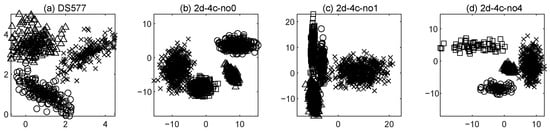
Figure 1. Four synthetic datasets. The shape of a point in the graph represents its sensitive attribute. (a) DS-577; (b) 2d-4c-no0; (c) 2d-4c-no1; (d) 2d-4c-no4.

4.2. Experimental Setup

To comprehensively evaluate the proposed method, we conducted experiments on both two-dimensional synthetic datasets and real-world datasets. We compared our approach against several baseline methods, including K-means, ensemble clustering methods (PFEC, LEGP [39], LEWA [39], ECPCS_MC [40], ECPCS_HC [40]), mainstream fair clustering algorithms (fair unnormalized spectral clustering (FSCUN) [29], fair normalized spectral clustering (FSCN) [29], fair algorithms for clustering (FAC) [28]), and the fair ensemble clustering method (FCE) proposed by Zhou et al. For our method, we constructed a pool of 100 base clusterings, generated by varying the initialization centroids of K-means and the number of clusters. The random seed for cluster center initialization was fixed at 2025. The number of clusters was sampled from the interval $\left[min\{c,\sqrt{n}\},max\{c,\sqrt{n}\}\right]$. In each trial, we randomly selected 20 base clusterings to execute our method, and repeated this process 10 times without parameter adjustments to compute the mean and variance. The optimal settings for the hyperparameters ${\lambda }_1$ and ${\lambda }_2$ were determined through a grid search. Comparative methods were configured according to their original recommended settings, with FCE utilizing K-means generated base clusterings. The details of our method and the comparative methods are summarized in Table 2.

Table 2. Comparison of clustering methods in terms of fairness consideration, fairness type, ensemble framework, and complexity.

Method	Fairness	Fairness Type	Ensemble?	Complexity
K-means	No	-	No	$O\left(nkdt\right)$
PFEC [6]	No	-	Yes	$O\left(n^{2}m\right)$
LWGP [39]	No	-	Yes	$O\left(nm\right)$
LWEA [39]	No	-	Yes	$O(n^{2}m+n^3)$
ECPCS-HC [40]	No	-	Yes	$O(n^{2}m+n^3)$
ECPCS-MC [40]	No	-	Yes	$O(n_c^3+n_{c}n)$
FSCUN [29]	Yes	Group	No	$O\left(n^3\right)$
FSCN [29]	Yes	Group	No	$O\left(n^3\right)$
FAC [28]	Yes	Group	No	$O\left(nkdt\right)$
FCE [32]	Yes	Group	Yes	$O\left(n^{2}m\right)$
Ours	Yes	Group	Yes	$O(n^{2}max\{c,m\})$

Note: $n_c$ refers to the total number of clusters from all base clusterings in the ensemble.

We employed four evaluation metrics: two external metrics (ACC and NMI) to measure the similarity between clustering results and ground truth labels, thus assessing clustering quality; one internal metric (SSE) to evaluate intra-cluster tightness; and two fairness metrics (BAL and MNCE) to quantify the balance of sensitive attribute distributions across clusters.

For each dataset, the ideal fair state is defined such that the proportion of each sensitive group within every cluster matches its global proportion in the entire dataset, i.e.,

$$pr\left({\mathcal{G}}_s\right|{\pi }_v)=pr\left({\mathcal{G}}_s\right)\forall s,v.$$

(46)

The BAL metric measures the balance between different sensitive groups within clusters, with higher values indicating more equitable distributions. Specifically, BAL is defined as the minimum ratio between the sizes of the smallest and largest sensitive groups in any cluster:

$$\mathrm{Bal}\left(C\right)=\underset{k}{min}\left({\displaystyle \frac{N_k^{min}}{N_k^{max}}}\right)\in [0,1],$$

(47)

where $N_k^{min}$ and $N_k^{max}$ represent the number of instances in the smallest and largest sensitive groups in cluster $C_k$, respectively. Values closer to 1 indicate fairer clustering results.

MNCE evaluates distributional imbalance by comparing the entropy of sensitive group distributions within clusters against the global entropy of sensitive group distributions:

$$MNCE=\underset{k}{min}\left({\displaystyle \frac{-{\sum }_i\frac{|P_i\cap C_k|}{|C_k|}log\frac{|P_i\cap C_k|}{|C_k|}}{-{\sum }_i\frac{|P_i|}{n}log\frac{|P_i|}{n}}}\right)\in [0,1],$$

(48)

where $|P_i\cap C_k|$ denotes the number of instances from the i-th sensitive group in cluster $C_k$, $|C_k|$ represents the total instances in cluster $C_k$, $|P_i|$ indicates the total instances in the i-th sensitive group, and n is the overall sample size. Higher MNCE values indicate better fairness by minimizing the unevenness of sensitive attribute distributions.

The convergence condition is set as: the relative change in the objective function value between two consecutive iterations is less than ${10}^{-6}$, or the maximum number of iterations $T_{max}=100$ is reached.

4.3. Experimental Results and Comparison

As shown in Figure 2, the proposed method introduces a fairness mechanism, which distinguishes it from the original ensemble clustering algorithm PFEC as well as several existing fair clustering algorithms. This mechanism ensures that the distribution of sensitive attributes within each cluster remains consistent with the global distribution. However, incorporating such fairness constraints inevitably affects clustering quality to some degree, a trade-off that becomes especially pronounced when the data distribution is highly correlated with sensitive attributes. For example, on several synthetic datasets, to obtain fairer outcomes, it was necessary to assign some geographically proximate points to different clusters so that the proportion of points possessing each sensitive attribute within every cluster matches the overall distribution. Our objective is to achieve relatively high clustering quality while maintaining strong fairness, keeping points within clusters more compactly grouped rather than sacrificing clustering performance entirely in pursuit of fairness. Empirical evidence from Table 3, Table 4, Table 5, Table 6 and Table 7 indicates that several fair clustering methods underperform on the two-dimensional datasets depicted in Figure 2 with respect to conventional clustering quality metrics. Notwithstanding this, they achieve superior performance in fairness metrics. Compared to the FCE algorithm, our method attains excellent fairness values on the DS577 dataset while simultaneously demonstrating advantages in terms of Accuracy (ACC), Normalized Mutual Information (NMI), and Sum of Squared Errors (SSE). Visual inspection of the results reveals that our method yields more compact and coherent clusters. On the 2d-4c-no0 and 2d-4c-no1 datasets, a marginal deficiency is observed in the fairness metrics of our method relative to FCE. It is noteworthy, however, that this minor discrepancy is attributable to only one or two outlier data points, thereby exerting a negligible impact on the overall results. Furthermore, our method maintains superior performance on standard clustering metrics. On the 2d-4c-no4 dataset, our approach comprehensively surpasses FCE across all evaluated metrics.

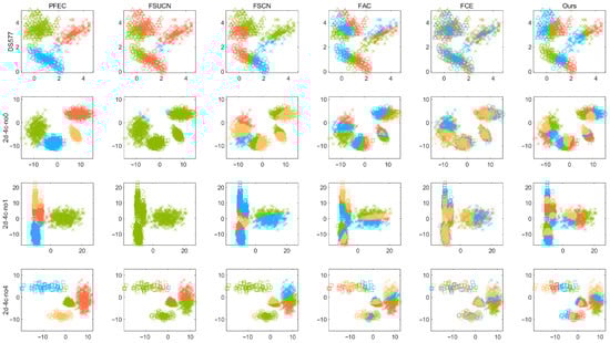
Figure 2. Clustering results on the synthetic datasets. Clusters are represented by different colors, and sensitive attributes are indicated by shapes.

Table 3. The ACC(%) values of our algorithm and the comparative algorithms (optimal values in bold, suboptimal values underlined).

Method	DS-577 (k = 3)	2d-4c-no0 (k = 4)	2d-4c-no1 (k = 4)	2d-4c-no4 (k = 4)	HAR (k = 6)	MNIST-USPS (k = 10)	Reverse MNIST (k = 10)	JAFFE (k = 10)
KM	$\mathbf{0}.\mathbf{999}\pm \mathbf{0}.\mathbf{001}$	$\underline{0.929\pm 0.138}$	$0.802\pm 0.107$	$0.846\pm 0.168$	$0.547\pm 0.067$	$0.322\pm 0.013$	$0.348\pm 0.008$	$0.743\pm 0.079$
PFEC	$0.982\pm 0.001$	$\mathbf{0}.\mathbf{998}\pm \mathbf{0}.\mathbf{001}$	$\underline{0.940\pm 0.032}$	$\underline{0.998\pm 0.001}$	$0.564\pm 0.015$	$0.368\pm 0.026$	$0.344\pm 0.005$	$0.801\pm 0.052$
LWGP	$0.967\pm 0.001$	$\mathbf{0}.\mathbf{998}\pm \mathbf{0}.\mathbf{001}$	$0.921\pm 0.088$	$\mathbf{0}.\mathbf{999}\pm \mathbf{0}.\mathbf{001}$	$0.562\pm 0.024$	$0.355\pm 0.021$	$0.348\pm 0.008$	$0.795\pm 0.051$
LWEA	$0.967\pm 0.001$	$0.997\pm 0.001$	$0.776\pm 0.092$	$0.982\pm 0.076$	$0.582\pm 0.022$	$0.381\pm 0.015$	$0.344\pm 0.012$	$0.802\pm 0.068$
ECPCS-HC	$0.968\pm 0.002$	$0.997\pm 0.001$	$0.938\pm 0.080$	$0.000\pm 0.000$	$0.579\pm 0.013$	$0.372\pm 0.019$	$0.297\pm 0.028$	$0.727\pm 0.058$
ECPCS-MC	$0.968\pm 0.001$	$\mathbf{0}.\mathbf{998}\pm \mathbf{0}.\mathbf{001}$	$0.906\pm 0.056$	$\mathbf{0}.\mathbf{999}\pm \mathbf{0}.\mathbf{001}$	$0.571\pm 0.017$	$0.369\pm 0.012$	$\underline{0.349\pm 0.006}$	$0.772\pm 0.059$
FSCUN	$0.464\pm 0.002$	$0.321\pm 0.000$	$0.332\pm 0.000$	$0.530\pm 0.000$	$0.471\pm 0.000$	$0.318\pm 0.009$	$0.110\pm 0.000$	$0.690\pm 0.000$
FSCN	$0.573\pm 0.029$	$0.353\pm 0.031$	$0.440\pm 0.012$	$0.382\pm 0.002$	$0.733\pm 0.005$	$0.282\pm 0.000$	$0.316\pm 0.001$	$\underline{0.967\pm 0.000}$
FAC	$0.452\pm 0.000$	$0.351\pm 0.000$	$0.338\pm 0.000$	$0.320\pm 0.000$	$\underline{0.742\pm 0.000}$	$0.274\pm 0.000$	$0.244\pm 0.000$	$0.817\pm 0.000$
FCE	$0.351\pm 0.006$	$0.252\pm 0.001$	$0.251\pm 0.000$	$0.255\pm 0.001$	$0.648\pm 0.026$	$\underline{0.419\pm 0.022}$	$0.359\pm 0.012$	$0.913\pm 0.086$
Ours	$0.362\pm 0.006$	$0.260\pm 0.002$	$0.265\pm 0.003$	$0.280\pm 0.014$	$\mathbf{0}.\mathbf{747}\pm \mathbf{0}.\mathbf{020}$	$\mathbf{0}.\mathbf{512}\pm \mathbf{0}.\mathbf{002}$	$\mathbf{0}.\mathbf{362}\pm \mathbf{0}.\mathbf{012}$	$\mathbf{0}.\mathbf{980}\pm \mathbf{0}.\mathbf{010}$

Table 4. The NMI(%) values of our algorithm and the comparative algorithms (optimal values in bold, suboptimal values underlined).

Method	DS-577 (k = 3)	2d-4c-no0 (k = 4)	2d-4c-no1 (k = 4)	2d-4c-no4 (k = 4)	HAR (k = 6)	MNIST-USPS (k = 10)	Reverse MNIST (k = 10)	JAFFE (k = 10)
KM	$\mathbf{0}.\mathbf{999}\pm \mathbf{0}.\mathbf{001}$	$\underline{0.943\pm 0.074}$	$0.810\pm 0.021$	$0.871\pm 0.117$	$0.572\pm 0.047$	$0.302\pm 0.011$	$0.285\pm 0.021$	$0.828\pm 0.053$
PFEC	$0.902\pm 0.002$	$\mathbf{0}.\mathbf{992}\pm \mathbf{0}.\mathbf{001}$	$\underline{0.934\pm 0.045}$	$\underline{0.994\pm 0.005}$	$0.586\pm 0.023$	$0.352\pm 0.010$	$0.368\pm 0.015$	$0.872\pm 0.029$
LWGP	$0.875\pm 0.003$	$0.990\pm 0.002$	$0.889\pm 0.064$	$\mathbf{0}.\mathbf{995}\pm \mathbf{0}.\mathbf{005}$	$0.588\pm 0.031$	$0.348\pm 0.009$	$0.362\pm 0.016$	$0.862\pm 0.027$
LWEA	$0.873\pm 0.003$	$0.989\pm 0.003$	$0.829\pm 0.055$	$0.981\pm 0.055$	$0.637\pm 0.023$	$0.345\pm 0.007$	$0.346\pm 0.021$	$0.869\pm 0.031$
ECPCS-HC	$0.876\pm 0.004$	$0.988\pm 0.003$	$0.908\pm 0.046$	$0.000\pm 0.000$	$0.668\pm 0.014$	$0.354\pm 0.009$	$0.244\pm 0.058$	$0.838\pm 0.031$
ECPCS-MC	$0.877\pm 0.002$	$\underline{0.993\pm 0.004}$	$0.854\pm 0.047$	$\mathbf{0}.\mathbf{997}\pm \mathbf{0}.\mathbf{005}$	$0.609\pm 0.029$	$0.357\pm 0.011$	$\underline{0.369\pm 0.005}$	$0.852\pm 0.032$
FSCUN	$0.138\pm 0.001$	$0.013\pm 0.000$	$0.003\pm 0.000$	$0.129\pm 0.000$	$0.571\pm 0.001$	$0.289\pm 0.004$	$0.005\pm 0.000$	$0.833\pm 0.000$
FSCN	$0.235\pm 0.041$	$0.170\pm 0.061$	$0.292\pm 0.031$	$0.243\pm 0.055$	$0.662\pm 0.002$	$0.308\pm 0.000$	$0.333\pm 0.000$	$\underline{0.964\pm 0.000}$
FAC	$0.028\pm 0.000$	$0.015\pm 0.000$	$0.012\pm 0.000$	$0.018\pm 0.000$	$\underline{0.669\pm 0.000}$	$0.199\pm 0.000$	$0.145\pm 0.000$	$0.854\pm 0.000$
FCE	$0.001\pm 0.001$	$0.000\pm 0.000$	$0.000\pm 0.000$	$0.000\pm 0.000$	$0.557\pm 0.024$	$0.385\pm 0.013$	$0.368\pm 0.02$	$0.896\pm 0.077$
Ours	$0.003\pm 0.001$	$0.000\pm 0.000$	$0.000\pm 0.000$	$0.000\pm 0.000$	$\mathbf{0}.\mathbf{672}\pm \mathbf{0}.\mathbf{041}$	$\mathbf{0}.\mathbf{436}\pm \mathbf{0}.\mathbf{002}$	$\mathbf{0}.\mathbf{372}\pm \mathbf{0}.\mathbf{005}$	$\mathbf{0}.\mathbf{974}\pm \mathbf{0}.\mathbf{028}$

Table 5. The SSE values of our algorithm and the comparative algorithms (optimal values in bold, suboptimal values underlined).

Method	DS-577 (k = 3)	2d-4c-no0 (k = 4)	2d-4c-no1 (k = 4)	2d-4c-no4 (k = 4)	HAR (k = 6)	MNIST-USPS (k = 10)	Reverse MNIST (k = 10)	JAFFE (k = 10)
KM	$\mathbf{71}.\mathbf{174}\pm \mathbf{0}.\mathbf{000}$	$\underline{147.465\pm 54.956}$	$\mathbf{125}.\mathbf{465}\pm \mathbf{18}.\mathbf{652}$	$\underline{180.639\pm 44.573}$	$\mathbf{421}.\mathbf{740}\pm \mathbf{2}.\mathbf{578}$	$\mathbf{1001}.\mathbf{484}\pm \mathbf{31}.\mathbf{012}$	$\mathbf{1081}.\mathbf{214}\pm \mathbf{6}.\mathbf{140}$	$\mathbf{64}.\mathbf{149}\pm \mathbf{0}.\mathbf{000}$
PFEC	$80.192\pm 1.673$	$\mathbf{122}.\mathbf{672}\pm \mathbf{0}.\mathbf{971}$	$132.554\pm 5.024$	$206.824\pm 0.891$	$432.891\pm 4.214$	$\underline{1034.583\pm 30.285}$	$\underline{1081.214\pm 6.140}$	$\underline{66.135\pm 2.150}$
LWGP	$81.918\pm 1.735$	$124.997\pm 0.751$	$174.803\pm 86.514$	$204.848\pm 0.857$	$428.527\pm 4.549$	$1100.592\pm 35.039$	$1110.103\pm 7.341$	$69.544\pm 2.520$
LWEA	$82.843\pm 1.707$	$125.150\pm 0.916$	$139.058\pm 11.391$	$200.652\pm 17.518$	$434.760\pm 5.986$	$1134.151\pm 10.653$	$1106.245\pm 5.876$	$68.684\pm 3.342$
ECPCS-HC	$81.352\pm 1.992$	$124.683\pm 1.547$	$135.679\pm 4.194$	$0.000\pm 0.000$	$436.780\pm 5.041$	$1146.345\pm 13.808$	$1097.999\pm 7.160$	$73.097\pm 3.203$
ECPCS-MC	$80.907\pm 1.207$	$124.222\pm 0.183$	$204.688\pm 114.886$	$204.645\pm 0.877$	$421.740\pm 2.578$	$1034.583\pm 30.285$	$1095.734\pm 7.134$	$70.917\pm 3.761$
FSCUN	$460.711\pm 0.836$	$1530.374\pm 0.000$	$1614.998\pm 0.000$	$634.852\pm 0.000$	$469.185\pm 0.050$	$1383.759\pm 16.756$	$3990.999\pm 0.000$	$73.416\pm 0.000$
FSCN	$395.266\pm 74.097$	$1243.533\pm 88.108$	$1111.799\pm 60.268$	$574.834\pm 39.023$	$423.147\pm 2.022$	$1157.652\pm 0.851$	$2207.682\pm 16.195$	$\mathbf{64}.\mathbf{149}\pm \mathbf{0}.\mathbf{000}$
FAC	$500.437\pm 0.000$	$1410.137\pm 0.000$	$1472.426\pm 0.000$	$674.395\pm 0.000$	$440.259\pm 0.000$	$3119.421\pm 0.000$	$3631.785\pm 0.000$	$76.735\pm 0.000$
FCE	$576.123\pm 0.474$	$1545.267\pm 0.147$	$1616.014\pm 0.764$	$847.566\pm 9.289$	$458.278\pm 2.116$	$3153.548\pm 10.013$	$3551.728\pm 5.189$	$74.148\pm 9.253$
Ours	$563.430\pm 4.513$	$1520.350\pm 6.269$	$1600.552\pm 2.669$	$799.761\pm 24.847$	$435.115\pm 12.101$	$3058.837\pm 0.912$	$3354.145\pm 3.890$	$71.832\pm 11.018$

Table 6. The BAL values of our algorithm and the comparative algorithms (optimal values in bold, suboptimal values underlined).

Method	DS-577 (k = 3)	2d-4c-no0 (k = 4)	2d-4c-no1 (k = 4)	2d-4c-no4 (k = 4)	HAR (k = 6)	MNIST-USPS (k = 10)	Reverse MNIST (k = 10)	JAFFE (k = 10)
KM	$0.000\pm 0.000$	$0.000\pm 0.000$	$0.000\pm 0.000$	$0.000\pm 0.000$	$0.000\pm 0.000$	$0.000\pm 0.000$	$0.000\pm 0.000$	$0.000\pm 0.000$
PFEC	$0.000\pm 0.000$	$0.000\pm 0.000$	$0.000\pm 0.000$	$0.000\pm 0.000$	$0.000\pm 0.000$	$0.000\pm 0.000$	$0.000\pm 0.000$	$0.000\pm 0.000$
LWGP	$0.000\pm 0.000$	$0.000\pm 0.000$	$0.000\pm 0.000$	$0.000\pm 0.000$	$0.000\pm 0.000$	$0.000\pm 0.000$	$0.000\pm 0.000$	$0.000\pm 0.000$
LWEA	$0.000\pm 0.000$	$0.000\pm 0.000$	$0.000\pm 0.000$	$0.000\pm 0.000$	$0.000\pm 0.000$	$0.000\pm 0.000$	$0.000\pm 0.000$	$0.000\pm 0.000$
ECPCS-HC	$0.000\pm 0.000$	$0.000\pm 0.000$	$0.000\pm 0.000$	$0.000\pm 0.000$	$0.000\pm 0.000$	$0.000\pm 0.000$	$0.000\pm 0.000$	$0.000\pm 0.000$
ECPCS-MC	$0.000\pm 0.000$	$0.000\pm 0.000$	$0.000\pm 0.000$	$0.000\pm 0.000$	$0.000\pm 0.000$	$0.000\pm 0.000$	$0.000\pm 0.000$	$0.000\pm 0.000$
FSCUN	$0.000\pm 0.000$	$0.000\pm 0.000$	$0.000\pm 0.000$	$0.000\pm 0.000$	$0.000\pm 0.000$	$0.000\pm 0.000$	$0.000\pm 0.000$	$0.000\pm 0.000$
FSCN	$0.000\pm 0.000$	$0.000\pm 0.000$	$0.000\pm 0.000$	$0.000\pm 0.000$	$0.000\pm 0.000$	$0.000\pm 0.000$	$0.000\pm 0.000$	$0.000\pm 0.000$
FAC	$\underline{0.600\pm 0.000}$	$\underline{0.329\pm 0.000}$	$\underline{0.233\pm 0.000}$	$\underline{0.095\pm 0.000}$	$0.000\pm 0.000$	$\underline{0.609\pm 0.000}$	$\underline{0.661\pm 0.000}$	$\underline{0.333\pm 0.000}$
FCE	$0.896\pm 0.000$	$0.515\pm 0.000$	$0.356\pm 0.000$	$0.142\pm 0.001$	$\underline{0.149\pm 0.148}$	$0.105\pm 0.037$	$0.339\pm 0.030$	$0.483\pm 0.032$
Ours	$\mathbf{0}.\mathbf{890}\pm \mathbf{0}.\mathbf{003}$	$\mathbf{0}.\mathbf{513}\pm \mathbf{0}.\mathbf{002}$	$\mathbf{0}.\mathbf{354}\pm \mathbf{0}.\mathbf{002}$	$\mathbf{0}.\mathbf{144}\pm \mathbf{0}.\mathbf{002}$	$\mathbf{0}.\mathbf{700}\pm \mathbf{0}.\mathbf{067}$	$\mathbf{0}.\mathbf{812}\pm \mathbf{0}.\mathbf{002}$	$\mathbf{0}.\mathbf{465}\pm \mathbf{0}.\mathbf{001}$	$\mathbf{0}.\mathbf{500}\pm \mathbf{0}.\mathbf{003}$

Table 7. The MNCE values of our algorithm and the comparative algorithms (optimal values in bold, suboptimal values underlined).

Method	DS-577 (k = 3)	2d-4c-no0 (k = 4)	2d-4c-no1 (k = 4)	2d-4c-no4 (k = 4)	HAR (k = 6)	MNIST-USPS (k = 10)	Reverse MNIST (k = 10)	JAFFE (k = 10)
KM	$\underline{0.054\pm 0.000}$	$0.000\pm 0.000$	$0.000\pm 0.000$	$0.000\pm 0.000$	$\underline{0.810\pm 0.113}$	$0.000\pm 0.000$	$0.000\pm 0.000$	$\underline{0.299\pm 0.290}$
PFEC	$0.000\pm 0.000$	$0.000\pm 0.000$	$0.000\pm 0.000$	$0.000\pm 0.000$	$0.620\pm 0.210$	$0.000\pm 0.000$	$0.000\pm 0.000$	$0.320\pm 0.304$
LWGP	$0.000\pm 0.000$	$0.000\pm 0.000$	$0.000\pm 0.000$	$0.000\pm 0.000$	$0.597\pm 0.166$	$0.000\pm 0.000$	$0.000\pm 0.000$	$0.301\pm 0.314$
LWEA	$0.000\pm 0.000$	$0.000\pm 0.000$	$0.000\pm 0.000$	$0.000\pm 0.000$	$0.610\pm 0.107$	$0.000\pm 0.000$	$0.000\pm 0.000$	$0.358\pm 0.329$
ECPCS-HC	$0.000\pm 0.000$	$0.000\pm 0.000$	$0.000\pm 0.000$	$0.000\pm 0.000$	$0.000\pm 0.000$	$0.000\pm 0.000$	$0.000\pm 0.000$	$0.000\pm 0.000$
ECPCS-MC	$0.000\pm 0.000$	$0.000\pm 0.000$	$0.000\pm 0.000$	$0.000\pm 0.000$	$0.841\pm 0.101$	$0.000\pm 0.000$	$0.000\pm 0.000$	$0.101\pm 0.213$
FSCUN	$0.000\pm 0.000$	$0.000\pm 0.000$	$0.000\pm 0.000$	$0.000\pm 0.000$	$0.000\pm 0.000$	$0.000\pm 0.000$	$0.000\pm 0.000$	$0.000\pm 0.000$
FSCN	$0.446\pm 0.235$	$0.000\pm 0.000$	$0.000\pm 0.000$	$0.000\pm 0.000$	$0.963\pm 0.000$	$0.000\pm 0.000$	$0.000\pm 0.000$	$0.896\pm 0.000$
FAC	$0.979\pm 0.000$	$0.961\pm 0.000$	$0.962\pm 0.000$	$0.905\pm 0.000$	$0.860\pm 0.000$	$0.959\pm 0.000$	$0.970\pm 0.000$	$0.970\pm 0.000$
FCE	$\mathbf{1}.\mathbf{000}\pm \mathbf{0}.\mathbf{000}$	$\mathbf{1}.\mathbf{000}\pm \mathbf{0}.\mathbf{000}$	$\mathbf{1}.\mathbf{000}\pm \mathbf{0}.\mathbf{000}$	$\underline{0.995\pm 0.003}$	$\underline{0.977\pm 0.002}$	$\underline{0.445\pm 0.094}$	$\underline{0.814\pm 0.027}$	$\underline{0.986\pm 0.005}$
Ours	$\mathbf{1}.\mathbf{000}\pm \mathbf{0}.\mathbf{000}$	$\underline{0.999\pm 0.000}$	$\mathbf{1}.\mathbf{000}\pm \mathbf{0}.\mathbf{000}$	$\mathbf{0}.\mathbf{998}\pm \mathbf{0}.\mathbf{001}$	$\mathbf{0}.\mathbf{998}\pm \mathbf{0}.\mathbf{001}$	$\mathbf{0}.\mathbf{978}\pm \mathbf{0}.\mathbf{003}$	$\mathbf{0}.\mathbf{902}\pm \mathbf{0}.\mathbf{002}$	$\mathbf{0}.\mathbf{989}\pm \mathbf{0}.\mathbf{009}$

The distribution of data points with sensitive attributes in real-world datasets often diverges significantly from the characteristics of synthetic datasets. As the results demonstrate, traditional algorithms such as K-means and ensemble methods including PFEC, LEGP, LEWA, ECPCS_MC, and ECPCS_HC yield comparatively poor results in terms of ACC and NMI on these real datasets. Additionally, the MNCE values on the HAR and JAFFE datasets are not uniformly zero, which contrasts with their performance on the two-dimensional datasets. This discrepancy suggests that the underlying data structures of these real-world datasets deviate from the property observed in two-dimensional data, where spatially proximate points typically share identical sensitive attributes. On these real-world datasets, our method not only achieves outstanding results in fairness metrics but also attains the best performance in external validation indices, namely ACC and NMI, outperforming all baseline algorithms. Although its performance on the SSE internal metric is inferior to that of standard clustering algorithms. It remains competitive when compared to other fair clustering approaches such as FSCUN, FSCN, FAC, and FCE. In summary, our method exhibits consistent improvements over FCE in both clustering quality and fairness enforcement. Table 8 presents the runtime of the proposed method on various datasets, demonstrating its computational efficiency under different data scales and complexities.

Table 8. Runtime of the Proposed Method on Various Datasets (Unit: seconds).

Dataset	Runtime
DS-577	0.012
2d-4c-no0	0.355
2d-4c-no1	0.326
2d-4c-no4	0.361
JAFFE	0.010

4.4. Sensitivity Analysis

To investigate the sensitivity of the model to key hyperparameters, we conducted a systematic sensitivity analysis on the regularization parameters ${\lambda }_1$ and ${\lambda }_2$. The experiment was carried out on several synthetic datasets and the real-world facial dataset JAFFE. By varying the values of ${\lambda }_1$ and ${\lambda }_2$, we observed their effects on the model’s classification accuracy (ACC) and balance (BAL). The experimental results are shown in Figure 3.

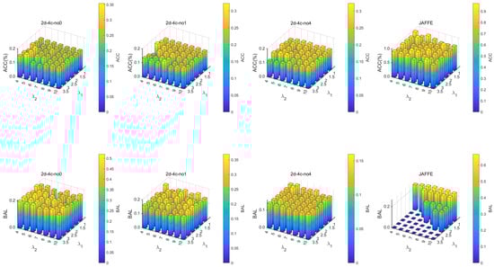
Figure 3. Sensitivity Analysis.

As can be seen from the figure, the model exhibits good robustness to changes in ${\lambda }_1$ and ${\lambda }_2$ on the synthetic datasets. Both ACC and BAL remain relatively stable under different parameter settings. This indicates that the synthetic data distributions are relatively uniform and the model is less dependent on fairness constraints.

However, on the real-world dataset JAFFE, the model’s performance shows a notably different trend. The results reveal that the BAL metric improves significantly only when ${\lambda }_2$ is set to a relatively large value, which corresponds to imposing a stronger fairness constraint, while ACC remains at a high level. This suggests that when dealing with real-world data bias, strengthening the fairness constraint is crucial for improving the fairness of model decisions. Therefore, in subsequent experiments on real-world datasets, we set ${\lambda }_2$ to a larger value to better balance model performance and fairness.

In summary, the sensitivity analysis not only verifies the stability of the model on synthetic data but also highlights the necessity of adjusting fairness constraints in real-world scenarios, providing an experimental basis for hyperparameter selection.

4.5. Ablation Study

To verify the practical effect of the fairness constraint in ensemble clustering, we conduct an ablation study to investigate its impact in real-world scenarios. HAR and MNIST-USPS are selected for the experiment, representing sensor-based activity recognition and cross-domain handwritten digit classification tasks, respectively. Both datasets possess clear sensitive attributes and inherent structural complexity, making them closer to actual application environments. In the objective function, the second constraint controlled by the parameter ${\lambda }_1$ plays a structural role and cannot be omitted; therefore, ${\lambda }_1>0$ is maintained in all experiments. This study mainly compares the full method (Ours) with a version that removes the fairness constraint. The results are summarized in Table 9. From the experimental outcomes, it can be observed that after introducing the fairness constraint, the fairness metrics BAL and MNCE on both datasets are significantly improved, indicating that the model can effectively promote a balanced distribution of each sensitive group in the clustering. Meanwhile, the clustering quality metrics ACC and NMI also show improvement on HAR and MNIST-USPS, suggesting that the fairness constraint does not harm the overall consistency of the clustering structure and may even bring some structural optimization due to the re-balancing of group distributions in real data. Notably, on the MNIST-USPS dataset, the SSE value increases after adding the fairness constraint, implying a slight decrease in intra-cluster compactness. This may stem from the inconsistency between the distribution of the sensitive attribute and the clustering structure in this dataset; the fairness constraint causes a slight perturbation to the original geometric structure when adjusting group proportions. Overall, the ablation study demonstrates that the introduced fairness constraint can notably enhance group fairness in clustering results and, in most cases, does not significantly degrade clustering quality. It may even lead to improved overall performance in real-world scenarios, indicating that the method achieves a good balance between fairness and clustering effectiveness, and possesses potential for practical applications.

Table 9. Ablation study of objective fuction.

Method	HAR					MNIST-USPS
	ACC (%)	NMI (%)	SSE	BAL	MNCE	ACC (%)	NMI (%)	SSE	BAL	MNCE
Without Fairness	$0.561\pm 0.020$	$0.579\pm 0.018$	$440.102\pm 4.512$	$0.000\pm 0.000$	$0.000\pm 0.000$	$0.360\pm 0.039$	$0.359\pm 0.021$	$1035.672\pm 28.938$	$0.000\pm 0.000$	$0.000\pm 0.000$
Ours	$0.747\pm 0.020$	$0.672\pm 0.041$	$435.115\pm 12.101$	$0.700\pm 0.067$	$0.998\pm 0.001$	$0.512\pm 0.002$	$0.436\pm 0.020$	$3058.837\pm 0.912$	$0.812\pm 0.002$	$0.978\pm 0.003$

5. Conclusions

In this paper, we have presented a fair ensemble clustering method that extends the framework of Nie et al. [6] by incorporating proportional fairness constraints. Our key contribution is the integration methodology, which embeds fairness directly into the ensemble objective and optimizes it jointly with clustering quality. By introducing a regularization term, it ensures that the distribution of protected groups within each cluster closely aligns with their overall distribution in the dataset while also balancing cluster sizes to prevent extreme imbalances. Unlike conventional post-processing techniques, this method embeds fairness constraints directly into the objective function and employs an iterative optimization strategy to achieve both group fairness and a high clustering quality. Experimental results demonstrate that the proposed approach consistently delivers robust and fair clustering outcomes across datasets of varying sizes, establishing a solid foundation for its application in fairness-sensitive domains. In future work, we will explore how fairness-related information is embedded within the similarity matrix. Specifically, we will investigate the underlying mechanisms that govern the presence and representation of fairness information in the matrix, with the goal of enhancing the interpretability and effectiveness of fairness-aware clustering methods. Nevertheless, our method primarily focuses on group fairness and may face challenges with extremely high-dimensional or large-scale data due to the iterative optimization of the label matrix. Future work could extend this framework to individual fairness notions or integrate fairness constraints into other ensemble mechanisms, such as graph-based or deep ensemble clustering frameworks.

References

- Jain, A.K.; Murty, M.N.; Flynn, P.J. Data clustering: A review. ACM Comput. Surv. (CSUR) 1999, 31, 264–323. [Google Scholar] [CrossRef]
- Wang, L.; Pan, C. Robust level set image segmentation via a local correntropy-based K-means clustering. Pattern Recognit. 2014, 47, 1917–1925. [Google Scholar] [CrossRef]
- Chen, D.; Lv, J.; Yi, Z. Graph Regularized Restricted Boltzmann Machine. IEEE Trans. Neural Netw. Learn. Syst. 2018, 29, 2651–2659. [Google Scholar] [CrossRef]
- Tunali, V.; Bilgin, T.; Camurcu, A. An improved clustering algorithm for text mining: Multi-cluster spherical K-Means. Int. Arab. J. Inf. Technol. (IAJIT) 2016, 13, 12–19. [Google Scholar]
- Zhang, M. Weighted clustering ensemble: A review. Pattern Recognit. 2022, 124, 108428. [Google Scholar] [CrossRef]
- Xie, F.; Nie, F.; Yu, W.; Li, X. Parameter-free ensemble clustering with dynamic weighting mechanism. Pattern Recognit. 2024, 151, 110389. [Google Scholar] [CrossRef]
- Fred, A.; Jain, A. Data clustering using evidence accumulation. In Proceedings of the International Conference on Pattern Recognition, Quebec City, QC, Canada, 11–15 August 2002; Volume 4, pp. 276–280. [Google Scholar] [CrossRef]
- Ayad, H.G.; Kamel, M.S. On voting-based consensus of cluster ensembles. Pattern Recognit. 2010, 43, 1943–1953. [Google Scholar] [CrossRef]
- Fred, A.L.; Jain, A.K. Combining multiple clusterings using evidence accumulation. IEEE Trans. Pattern Anal. Mach. Intell. 2005, 27, 835–850. [Google Scholar] [CrossRef]
- Huang, D.; Wang, C.D.; Wu, J.S.; Lai, J.H.; Kwoh, C.K. Ultra-Scalable Spectral Clustering and Ensemble Clustering. IEEE Trans. Knowl. Data Eng. 2020, 32, 1212–1226. [Google Scholar] [CrossRef]
- Jia, Y.; Liu, H.; Hou, J.; Zhang, Q. Clustering ensemble meets low-rank tensor approximation. In Proceedings of the AAAI Conference on Artificial Intelligence, Online, 2–9 February 2021; Volume 35, pp. 7970–7978. [Google Scholar]
- Wang, T. CA-Tree: A hierarchical structure for efficient and scalable coassociation-based cluster ensembles. IEEE Trans. Syst. Man, Cybern. Part B (Cybern.) 2010, 41, 686–698. [Google Scholar] [CrossRef]
- Cai, Y.; Mahmud, M.S.; Xu, J.; Sun, X.; Huang, J.Z. Spectral ensemble clustering with doubly stochastic co-association matrix. Inf. Sci. 2025, 686, 121314. [Google Scholar] [CrossRef]
- Wu, Y.; Wu, R.; Liu, J.; Tang, X. Metawce: Learning to weight for weighted cluster ensemble. Inf. Sci. 2023, 629, 39–61. [Google Scholar] [CrossRef]
- Jia, Y.; Tao, S.; Wang, R.; Wang, Y. Ensemble Clustering via Co-Association Matrix Self-Enhancement. IEEE Trans. Neural Netw. Learn. Syst. 2024, 35, 11168–11179. [Google Scholar] [CrossRef] [PubMed]
- Zhou, P.; Du, L.; Shen, Y.D.; Li, X. Tri-level robust clustering ensemble with multiple graph learning. In Proceedings of the AAAI Conference on Artificial Intelligence, Online, 2–9 February 2021; Volume 35, pp. 11125–11133. [Google Scholar]
- Chen, M.S.; Lin, J.Q.; Wang, C.D.; Xi, W.D.; Huang, D. On regularizing multiple clusterings for ensemble clustering by graph tensor learning. In Proceedings of the 31st ACM International Conference on Multimedia, Ottawa, ON, Canada, 29 October–3 November 2023; pp. 3069–3077. [Google Scholar]
- Zhou, P.; Du, L.; Li, X. Self-paced consensus clustering with bipartite graph. In Proceedings of the 29th International Conference on International Joint Conferences on Artificial Intelligence, Macao, China, 19–25 August 2021; pp. 2133–2139. [Google Scholar]
- Yang, X.; Zhao, W.; Wang, J.; Peng, S.; Nie, F. Auto-weighted Graph Reconstruction for efficient ensemble clustering. Inf. Sci. 2025, 689, 121486. [Google Scholar] [CrossRef]
- Bian, Z.; Yu, L.; Qu, J.; Deng, Z.; Wang, S. An Ensemble Clustering Method via Learning the CA Matrix with Fuzzy Neighbors. Inf. Fusion 2025, 120, 103105. [Google Scholar] [CrossRef]
- Bai, L.; Liang, J.; Cao, F. A multiple k-means clustering ensemble algorithm to find nonlinearly separable clusters. Inf. Fusion 2020, 61, 36–47. [Google Scholar] [CrossRef]
- Zhang, R.; Hang, S.; Sun, Z.; Nie, F.; Wang, R.; Li, X. Anchor-based fast spectral ensemble clustering. Inf. Fusion 2025, 113, 102587. [Google Scholar] [CrossRef]
- Huang, D.; Wang, C.D.; Lai, J.H. Fast multi-view clustering via ensembles: Towards scalability, superiority, and simplicity. IEEE Trans. Knowl. Data Eng. 2023, 35, 11388–11402. [Google Scholar] [CrossRef]
- Mehrabi, N.; Morstatter, F.; Saxena, N.; Lerman, K.; Galstyan, A. A survey on bias and fairness in machine learning. ACM Comput. Surv. (CSUR) 2021, 54, 1–35. [Google Scholar] [CrossRef]
- Caton, S.; Haas, C. Fairness in machine learning: A survey. ACM Comput. Surv. 2024, 56, 1–38. [Google Scholar] [CrossRef]
- Chierichetti, F.; Kumar, R.; Lattanzi, S.; Vassilvitskii, S. Fair clustering through fairlets. In Proceedings of the 31st International Conference on Neural Information Processing Systems, Long Beach, CA, USA, 4–9 December 2017; Volume 30. [Google Scholar]
- Backurs, A.; Indyk, P.; Onak, K.; Schieber, B.; Vakilian, A.; Wagner, T. Scalable fair clustering. In Proceedings of the International Conference on Machine Learning, Long Beach, CA, USA, 9–15 June 2019; pp. 405–413. [Google Scholar]
- Bera, S.; Chakrabarty, D.; Flores, N.; Negahbani, M. Fair algorithms for clustering. In Proceedings of the Advances in Neural Information Processing Systems, Vancouver, BC, Canada, 8–14 December 2019; Volume 32. [Google Scholar]
- Kleindessner, M.; Samadi, S.; Awasthi, P.; Morgenstern, J. Guarantees for spectral clustering with fairness constraints. In Proceedings of the International Conference on Machine Learning, Long Beach, CA, USA, 9–15 June 2019; pp. 3458–3467. [Google Scholar]
- Ghadiri, M.; Samadi, S.; Vempala, S. Socially fair k-means clustering. In Proceedings of the ACM Conference on Fairness, Accountability, and Transparency, Online, 3–10 March 2021; pp. 438–448. [Google Scholar]
- Kleindessner, M.; Awasthi, P.; Morgenstern, J. Fair k-center clustering for data summarization. In Proceedings of the International Conference on Machine Learning, Long Beach, CA, USA, 9–15 June 2019; pp. 3448–3457. [Google Scholar]
- Zhou, P.; Li, R.; Ling, Z.; Du, L.; Liu, X. Fair Clustering Ensemble With Equal Cluster Capacity. IEEE Trans. Pattern Anal. Mach. Intell. 2024, 47, 1729–1746. [Google Scholar] [CrossRef] [PubMed]
- Fan, K. On a theorem of Weyl concerning eigenvalues of linear transformations I. Proc. Natl. Acad. Sci. USA 1949, 35, 652–655. [Google Scholar] [CrossRef] [PubMed]
- Shi, J.; Malik, J. Normalized cuts and image segmentation. IEEE Trans. Pattern Anal. Mach. Intell. 2000, 22, 888–905. [Google Scholar] [CrossRef]
- Nie, F.; Lu, J.; Wu, D.; Wang, R.; Li, X. A novel normalized-cut solver with nearest neighbor hierarchical initialization. IEEE Trans. Pattern Anal. Mach. Intell. 2023, 46, 659–666. [Google Scholar] [CrossRef]
- Anguita, D.; Ghio, A.; Oneto, L.; Parra, X.; Reyes-Ortiz, J.L. A public domain dataset for human activity recognition using smartphones. In Proceedings of the European Symposium on Artificial Neural Networks (ESANN), Bruges, Belgium, 24–26 April 2013; Volume 3, pp. 3–4. [Google Scholar]
- Li, P.; Zhao, H.; Liu, H. Deep fair clustering for visual learning. In Proceedings of the IEEE/CVF Conference on Computer Vision and Pattern Recognition, Seattle, WA, USA, 14–19 June 2020; pp. 9070–9079. [Google Scholar]
- Lyons, M.J.; Akamatsu, S.; Kamachi, M.; Gyoba, J.; Budynek, J. The Japanese female facial expression (JAFFE) database. In Proceedings of the 3rd International Conference on Automatic Face and Gesture Recognition, Nara, Japan, 14–16 April 1998; pp. 14–16. [Google Scholar]
- Huang, D.; Wang, C.D.; Lai, J.H. Locally weighted ensemble clustering. IEEE Trans. Cybern. 2017, 48, 1460–1473. [Google Scholar] [CrossRef]
- Huang, D.; Wang, C.D.; Peng, H.; Lai, J.; Kwoh, C.K. Enhanced ensemble clustering via fast propagation of cluster-wise similarities. IEEE Trans. Syst. Man Cybern. Syst. 2018, 51, 508–520. [Google Scholar] [CrossRef]
Disclaimer/Publisher’s Note: The statements, opinions and data contained in all publications are solely those of the individual author(s) and contributor(s) and not of MDPI and/or the editor(s). MDPI and/or the editor(s) disclaim responsibility for any injury to people or property resulting from any ideas, methods, instructions or products referred to in the content. |
© 2025 by the authors. Licensee MDPI, Basel, Switzerland. This article is an open access article distributed under the terms and conditions of the Creative Commons Attribution (CC BY) license (https://creativecommons.org/licenses/by/4.0/).