A New Flexible Integrated Linear–Weibull Lifetime Model: Analytical Characterization and Real-Data Studies

Abstract

In this work, we introduce a new four-parameter distribution, called the integrated linear–Weibull (ILW) model, constructed by embedding a dynamic linear component within the Weibull framework. The ILW distribution is capable of capturing a wide variety of symmetric and asymmetric density shapes and accommodates diverse failure-rate behaviors. We derive several of its key mathematical and statistical properties, including moments, extropy, cumulative residual entropy, order statistics, and their asymptotic forms. The mean residual life function and its reciprocal relationship with the failure rate are also obtained. An algorithm for generating random samples from the ILW distribution is provided, and model identifiability is examined numerically through the Kullback–Leibler divergence. Parameter estimation is carried out via maximum likelihood, and a simulation study is conducted to assess the accuracy of the estimators; the results show improvements in estimator performance as sample size increases. Finally, three real datasets involving failure-time observations and one describing hydrological and epidemiological data are analyzed to demonstrate the practical usefulness of the ILW model. In these applications, the proposed model exhibits competitive or superior performance relative to several existing lifetime distributions based on standard model selection criteria and goodness-of-fit measures.

1. Introduction

The Weibull distribution has emerged as a useful statistical model in the past decades, applied across a range of disciplines, including reliability engineering, biomedical sciences, economics, probability theory, and statistical mechanics. Its utility spans numerous practical contexts, from assessing product life spans to characterizing particle behaviors in physical systems and modeling survival data in medical research. As highlighted by [1], the Weibull distribution plays a role in capturing the variability in lifetimes among different products in real-world assessments. Likewise, ref. [2] shows its adaptability and relevance across various scientific domains. Despite its uses, the classical Weibull distribution has many limitations. A central weakness is its restricted ability to represent diverse data behaviors. In particular, the W density admits relatively few shapes and often fails to adequately capture highly right-skewed datasets, other asymmetric density shapes, heavy tails, and multimodal characteristics [3] (p. 282). Similarly, its mean residual life (MRL) function is limited in form and cannot accommodate the wide variety of patterns observed in practice, especially non-monotonic MRL [4] (Subsection 3.1). These drawbacks reduce the model’s flexibility and can lead to poor fit and poor statistical analysis when applied to complex real-world datasets, especially those with non-monotonic hazard rates (see [5] (Table 1) and [3]).

The complexity of modern data has therefore driven a growing emphasis on more flexible statistical models that can overcome these complexity shortcomings. In many applications, traditional models frequently struggle to accurately capture datasets characterized by features such as skewness, fat tails, multiple modes, or complex hazard rate structures that deviate from monotonicity. These features can significantly impact the accuracy and interpretability of statistical analysis. The development of extended or generalized distributions becomes essential. Such innovations enable statisticians to construct models that align more closely with empirical data, thereby improving inferential accuracy and predictive performance. Extending classical distributions can be viewed as formulating new data-generating processes, opening pathways to novel case studies, practical insights, and computational and theoretical studies. This approach enhances our analytical capabilities across sectors, including engineering, economics, biomedicine, etc. By enriching the toolbox of statistical modeling, extended distributions offer greater adaptability and robustness in the face of evolving data complexities. Ultimately, this forward-looking strategy ensures that statistical methodologies remain both rigorous and responsive to the demands of modern research. One of the classical models we intend to improve is the W, whose survival function is

$$s^{\ast }\left(x\right)=e^{-\alpha x^{\beta }},x,\alpha ,\beta >0.$$

(1)

Some W-related models derived from other methodologies over the last decade include the exponentiated additive-W [6], new extended-W [7], extended-W [8], extended exponential-W [9], odd flexible W-W [10], Q-W distribution [11], improved W-W [12], flexible Dhillon-W [13], hybrid W-Inverse-W [14], hybrid Weibull exponential [15], new modified exponent power alpha-W [16], and new tangent flexible-W [17], among others.

Given the wide-ranging nature of real-world datasets, each arising from distinct underlying processes and the increasing complexity of modern data, it is necessary to provide adaptable statistical models that can offer accurate and reliable analysis. Developing such flexible and dynamic models remains a critical challenge, as it requires the capacity to incorporate new structural features observed in empirical data. A well-designed model must not only accommodate these variations but also support robust forecasting and interpretation across diverse application domains. Thus, we propose a new four-parameter extension of the Weibull called the integrated linear–Weibull (ILW) distribution, capable of accommodating various shapes of densities, survival functions, and failure rate behaviors, while addressing the classical Weibull’s weaknesses in skewness and residual life representation.

Objectives and Paper Structure

The aim of this work is to introduce a novel integrated linear–Weibull model (ILW) that serves as a robust alternative for both theoretical exploration and practical applications. This model embeds its cumulative distribution function (CDF) into a dynamic linear–exponential structure. The inclusion of two linear parameters provides the model with additional flexibility to capture a wide variety of shapes for the density and hazard functions. The ILW distribution is capable of accommodating diverse tail behaviors and non-monotonic hazard structures. The ILW has four parameters, enabling it to model both symmetric and asymmetric density shapes, providing flexibility to fit a wide range of data patterns. This dynamic adaptability makes it a powerful tool for modeling lifetime data in reliability studies, life sciences, and other applications requiring flexible statistical models.

Secondly, its key statistical properties and potential applications are thoroughly examined, including the derivation of moments and information-theoretic measures, as well as the mean residual life, order statistics, and their asymptotic behavior. Furthermore, the model’s identifiability is assessed numerically using the Kullback–Leibler divergence. In addition, the reliability parameter is derived under the assumption of two independent variables.

Finally, we show that the model facilitates improving probabilistic modeling and data simulation. Maximum likelihood estimation (MLE) is considered for parameter inference, and its performance is evaluated through comprehensive simulation studies. The practical significance of the proposed model is shown via three real-world datasets.

This paper is outlined as follows: Section 2 details the introduction of the proposed model and discusses its valuable attributes, including moments, mean residual life, extropy, cumulative residual entropy, order statistics, the model’s identifiability, and the stress–strength parameter. Section 3 covers MLE and simulation experiments. Section 4 shows the application of the model through practical examples. This paper concludes in Section 5.

2. Model Definition and Properties

In this section, we define the proposed model. In addition, we derive some important model properties and measures, such as the quantile function, moments, extropy and cumulative residual entropy, order statistics and their asymptotic, mean residual life characteristics, model identifiability, and the reliability parameter.

2.1. Model Definition

Recently, ref. [15] proposed a methodology for extending distributions defined by

$$F^{\ast }(x;\xi ,\zeta )=1-e^{-w(x;\xi )G(x;\zeta )}.$$

(2)

where $G(x;\zeta )\in (0,1)$ is any valid CDF with $\zeta$ as a parameter vector in ${\mathbb{R}}^n$. $w(x;\xi )\in (c,\infty )$ is an increasing function with $c\ge 0$ and $\xi$ as its parameter vector in ${\mathbb{R}}^n$. Here, we consider $G(x;\zeta )$ to be a W model and an increasing function defined on $(b,\infty )$ with $b\ge 0$ as $(ax+b).$ By choosing a generalized linear function and following the hybrid family setting in (2), the proposed model CDF is derived by incorporating a dynamic linear structure with the W distribution CDF on an exponential framework:

$$F\left(x\right)=1-e^{-(ax+b)(1-e^{-\alpha x^{\beta }})}.$$

(3)

The corresponding probability density function (PDF), failure rate function (FRF), and survival function (SF) of the proposed model are, respectively, defined as follows:

$$\begin{array}{cc}\hfill f\left(x\right)& =[a(1-e^{-\alpha x^{\beta }})+\alpha \beta (ax+b)x^{\beta -1}{e}^{-\alpha x^{\beta }}]e^{-(ax+b)(1-e^{-\alpha x^{\beta }})},\hfill \end{array}$$

(4)

$$\begin{array}{cc}\hfill h\left(x\right)& =[a(1-e^{-\alpha x^{\beta }})+\alpha \beta (ax+b)x^{\beta -1}{e}^{-\alpha x^{\beta }}],\hfill \end{array}$$

(5)

$$\begin{array}{cc}\hfill s\left(x\right)& =e^{-(ax+b)(1-e^{-\alpha x^{\beta }})}.\hfill \end{array}$$

(6)

Figure 1 demonstrates some shapes of the PDF and FRF under different parameter settings. As depicted, the proposed model exhibits a high degree of flexibility in its FRF, which has decreasing, increasing, unimodal, or bathtub-shaped forms.

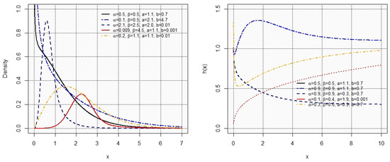
Figure 1. Plots of PDF and FRF of proposed model.

Theorem 1.

The FRF in (5) is unimodal at $x_0={\displaystyle \frac{2a-b\alpha }{a\alpha }},$ for ${\displaystyle \frac{b\alpha }{a}}<2$ and $\beta =1.$

Proof. 

This can be proved using the analysis of $h^{\prime }\left(x\right)$ as

$$h^{\prime }\left(x\right)=\alpha \beta x^{\beta -2}{e}^{-\alpha x^{\beta }}[2ax+(\beta -1)(ax+b)-\alpha \beta (ax+b)x^{\beta }],$$

The root can be obtain by solving

$$2ax+(\beta -1)(ax+b)-\alpha \beta (ax+b)x^{\beta }=0,$$

but it has many roots. To obtain at least one root, let $\beta =1$; hence,

$$2ax-\alpha x(ax+b)=0;\Rightarrow x_0={\displaystyle \frac{2a-b\alpha }{a\alpha }},$$

and ${\displaystyle \frac{b\alpha }{a}}<2.$    □

2.2. Quantile and Data Sampling Process

To simulate datasets from the proposed distribution, alternative sampling strategies are required due to the absence of a closed-form quantile function. The quantile function, denoted as $q\left(u\right)$, plays a fundamental role in random variate generation and subsequent statistical inference. Although the Markov Chain Monte Carlo (MCMC) approach remains a viable method, we also provide a direct numerical technique to approximate $q\left(u\right)$. Specifically, based on the CDF defined in (3), the $q\left(u\right)=X$ can be determine numerically solving the following:

$$F\left(X\right)=u,$$

where $u\in (0,1)$ follows a uniform distribution and $F(·)$ is the CDF of the proposed model. This root-finding approach facilitates efficient sampling, which is particularly useful for simulation studies and Monte Carlo-based inference. A uniroot function in the HDInterval package [18] in R-software (version 4.3.2) can be used to obtain the solution.

$$log[1-u]=(ax+b)(e^{-\alpha x^{\beta }}-1).$$

(7)

To simulate random samples from the proposed model, a practical algorithmic procedure is outlined in Algorithm 1 using Equation (7), as detailed below. Table 1 reports the first quartile, median, and third quartile for selected parameter values. For small parameter values (e.g., $\alpha =0.1,\beta =a=b=0.5$), the distribution is highly dispersed, with wide gaps between quartiles ($q\left(0.25\right)=1.42$, $q\left(0.5\right)=5.19$, and $q\left(0.75\right)=11.88$). As the parameters increase toward unity, the quartiles contract markedly, indicating a reduction in spread and a more concentrated distribution. For moderate values ($\alpha =\beta =a=b\approx$ 3 to 8.5), the quartiles remain close, with interquartile ranges below $0.2$, showing a stable and tightly centered distribution. At very large parameter values ($\alpha =\beta =a=b=20.5$), the quartiles are clustered even more tightly ($0.68$, $0.71$, and $0.74$), confirming the progressive concentration around the center. Overall, the results show that increasing the parameter values reduces dispersion and leads to a more symmetric and peaked distribution.

Table 1. Numerical values of the first quartile, median, and third quartile for some parameter values.

$\mathit{\alpha }$	$\mathit{\beta }$	a	b	$\mathit{q}\left(0.25\right)$	$\mathit{q}\left(0.5\right)$	$\mathit{q}\left(0.75\right)$
0.1	0.5	0.5	0.5	1.41577	5.19331	11.87559
0.5	0.5	0.5	0.5	0.69146	1.82367	3.54559
0.6	0.6	0.6	0.6	0.48655	1.29402	2.550117
0.7	0.7	0.7	0.7	0.37790	0.98320	1.94591
0.8	0.8	0.8	0.8	0.316806	0.78934	1.55148
0.9	0.9	0.9	0.9	0.28094	0.66318	1.288106
1.0	1.0	1.0	1.0	0.25935	0.5783	1.08926
1.1	1.1	1.1	1.1	0.24632	0.51975	0.94983
1.2	1.2	1.2	1.2	0.23871	0.47846	0.84652
1.5	1.5	1.5	1.5	0.23330	0.41185	0.66361
2.5	2.5	2.5	2.5	0.27029	0.38106	5.50746
3.0	3.0	3.0	3.0	0.29491	0.39252	0.49734
3.5	3.5	3.5	3.5	0.31923	0.40782	0.49885
5.5	5.5	5.5	5.5	0.40463	0.47289	0.53659
7.5	7.5	7.5	7.5	0.47090	0.52805	0.57901
8.5	8.5	8.5	8.5	0.49839	0.55146	0.59808
10.5	10.5	10.5	10.5	0.54492	0.59153	0.631165
12.5	12.5	12.5	12.5	0.58279	0.62445	0.65981
15.2	12.5	12.5	12.5	0.62806	0.66412	0.69429
20.5	20.5	20.5	20.5	0.68343	0.71296	0.73735

Algorithm 1. Generating random samples from the proposed model.

Step 1:     Specify the parameter values $\alpha$, $\beta$, a, and b.

Step 2:     Generate a random sample $u_i\sim \mathcal{U}(0,1)$ for $i=1,2,\dots ,n$.

Step 3:     For each $u_i$, numerically solve the following equation for $x_i$:                        $log(1-u_i)-(a{x}_i+b)\left(e^{-\alpha x_i^{\beta }}-1\right)=0$.

Bowley’s skewness (Bo) and Moor’s kurtosis (Mo) depend on model quantiles, making them well-suited for describing the distributional characteristics of the proposed model. Therefore, the skewness and kurtosis of the model can be analyzed using these quantile-based functions (see [15]). Figure 2 illustrates that for fixed values of $\alpha =1,b=1$, the skewness decreases as both $\beta$ and a increase. Similarly, the kurtosis also exhibits a decreasing trend with increasing values of $\beta$ and $a.$

Figure 2. Graphical presentation of the Bo (left) and Mo (right) for the proposed model.

2.3. Moment Characteristics

The $r^{th}$ moments of the proposed model offer insights into various statistical characteristics. Moments are essential for parameter estimation, model comparison, and deriving higher-order statistical properties in both theoretical and applied analysis. Lemma 1 is important for several computations of the model characteristics.

Lemma 1

([19] (p. 347)). Let $v>0,\beta >0,n>0$; then,

$${\int }_0^{\infty }{x}^m{e}^{-\beta x^n}dx={\displaystyle \frac{\gamma (v,\beta w^n)+\Gamma (v,\beta w^n)}{n{\beta }^v}},forsomew>0.$$

(8)

where $v={\displaystyle \frac{m+1}{n}};$$\Gamma (.,.)$ and $\gamma (.,.)$ are the upper and lower incomplete gamma functions, respectively.

The moments for the proposed model are computed as follows:

$$\begin{array}{cc}\hfill & E\left[X^r\right]={\int }_0^{\infty }{x}^r\left[a(1-e^{-\alpha x^{\beta }})+\alpha \beta (ax+b)x^{\beta -1}{e}^{-\alpha x^{\beta }}\right]e^{-(ax+b)(1-e^{-\alpha x^{\beta }})}dx,\hfill \\ \hfill & =a{\int }_0^{\infty }{x}^r(1-e^{-\alpha x^{\beta }})e^{-(ax+b)(1-e^{-\alpha x^{\beta }})}dx+\alpha \beta {\int }_0^{\infty }{x}^{r+\beta -1}(ax+b)e^{-\alpha x^{\beta }}{e}^{-(ax+b)(1-e^{-\alpha x^{\beta }})}dx.\hfill \end{array}$$

(9)

By applying binomial expansion and exponential expansion, we get the first integrand as

$$\begin{array}{cc}\hfill & a{x}^r(1-e^{-\alpha x^{\beta }})e^{-(ax+b)(1-e^{-\alpha x^{\beta }})}=a{x}^r\sum _{i=0}^{\infty }{\displaystyle \frac{{(-1)}^i}{i!}}{(ax+b)}^i{(1-e^{-\alpha x^{\beta }})}^{i+1}\hfill \\ \hfill & =\sum _{i=0}^{\infty }\sum _{j=0}^i\sum _{k=0}^{i+1}{\displaystyle \frac{{(-1)}^{i+k}{a}^{j+1}{b}^{i-j}}{i!}}\left(\genfrac{}{}{0pt}{}{i}{j}\right)\left(\genfrac{}{}{0pt}{}{i+1}{k}\right)x^{j+r}{e}^{-\alpha k{x}^{\beta }},\hfill \end{array}$$

while the second integrand is

$$\begin{array}{cc}\hfill & \alpha \beta x^{r+\beta -1}(ax+b)e^{-\alpha x^{\beta }}{e}^{-(ax+b)(1-e^{-\alpha x^{\beta }})}=\alpha \beta x^{r+\beta -1}{e}^{-\alpha x^{\beta }}\sum _{i=0}^{\infty }{\displaystyle \frac{{(-1)}^i}{i!}}{(ax+b)}^{i+1}{(1-e^{-\alpha x^{\beta }})}^i\hfill \\ \hfill & =\sum _{i=0}^{\infty }\sum _{j=0}^i\sum _{k=0}^{i+1}{\displaystyle \frac{{(-1)}^{i+j}\alpha \beta a^k{b}^{i+1-k}}{i!}}\left(\genfrac{}{}{0pt}{}{i}{j}\right)\left(\genfrac{}{}{0pt}{}{i+1}{k}\right)x^{k+r+\beta -1}{e}^{-\alpha (j+1)x^{\beta }}\hfill \end{array}$$

Thus, by putting back the integrands in series form in (9), we have

$$\begin{array}{cc}\hfill E\left[X^r\right]& =\sum _{i=0}^{\infty }\sum _{j=0}^i\sum _{k=0}^{i+1}{\tau }_{i,j,k}^{\left(1\right)}{\int }_0^{\infty }{x}^{j+r}{e}^{-\alpha k{x}^{\beta }}dx\hfill \\ \hfill & +\sum _{i=0}^{\infty }\sum _{j=0}^i\sum _{k=0}^{i+1}{\tau }_{i,k}^{\left(2\right)}{\int }_0^{\infty }{x}^{k+r+\beta -1}{e}^{-\alpha (j+1)x^{\beta }}dx.\hfill \end{array}$$

(10)

Then, applying Lemma 1, we arrive at

$$\begin{array}{cc}\hfill E\left[X^r\right]& =\sum _{i=0}^{\infty }\sum _{j=0}^i\sum _{k=0}^{i+1}{\tau }_{i,j,k}^{\left(1\right)}\left({\displaystyle \frac{\gamma (v,\alpha k{u}^{\beta })+\Gamma (v,\alpha k{u}^{\beta })}{\beta {\left(\alpha k\right)}^v}}\right)\hfill \\ \hfill & +\sum _{i=0}^{\infty }\sum _{j=0}^i\sum _{k=0}^{i+1}{\tau }_{i,k}^{\left(2\right)}\left({\displaystyle \frac{\gamma (z,\alpha (j+1)u^{\beta })+\Gamma (z,\alpha (j+1)u^{\beta })}{\beta {\left(\alpha (j+1)\right)}^z}}\right).\hfill \end{array}$$

(11)

for $u>0,$ where $v={\displaystyle \frac{r+j+1}{\beta }},$$z={\displaystyle \frac{r+k+\beta }{\beta }},$${\tau }_{i,j,k}^{\left(1\right)}={\displaystyle \frac{{(-1)}^{i+k}}{i!}}{b}^{i-j}{a}^{j+1}\left(\genfrac{}{}{0pt}{}{i}{j}\right)\left(\genfrac{}{}{0pt}{}{i+1}{k}\right),$ and ${\tau }_{i,k}^{\left(2\right)}={\displaystyle \frac{{(-1)}^{i+j}}{i!}}\alpha \beta b^{i+1-k}{a}^k\left(\genfrac{}{}{0pt}{}{i}{j}\right)\left(\genfrac{}{}{0pt}{}{i+1}{k}\right).$

Table 2 presents numerical values of the first four raw moments for selected parameter combinations. For small parameter values ($\alpha =0.5,\beta =0.5$), the distribution exhibits heavy tails, reflected in extremely large higher-order moments. As the parameters increase, the moments decrease substantially, indicating a lighter tail and greater concentration of the distribution. For larger settings ($\alpha \ge 1.5$), the first four moments are relatively close, suggesting that the distribution becomes sharply peaked with limited variability. The mean $\left(E\right[X\left]\right)$ and variance $(Var=E\left[X^2\right]-{\left(E\left[X\right]\right)}^2)$ of the proposed model are determined by setting $r=1$ and $r=2$, respectively, as outlined in (10). Figure 3 illustrates that for a fixed $\alpha =b=1,$ the mean of the proposed model decreases as the parameters $\beta$ and a increase. Conversely, the variance of the model initially increases and then significantly decreases as both $\beta$ and a increase.

Table 2. Numerical values of the first four moments for some parameter values.

$\mathit{\alpha }$	$\mathit{\beta }$	a	b	$\mathit{E}\left(\mathit{X}\right)$	$\mathit{E}\left({\mathit{X}}^2\right)$	$\mathit{E} \left({\mathit{X}}^3\right)$	$\mathit{E} \left({\mathit{X}}^4\right)$
0.5	0.5	0.5	0.1	2.86093	12.36907	83.57989	738.9234
		1.0	0.2	1.90111	4.29352	14.96601	70.97785
		1.5	0.3	1.58413	2.55573	5.92928	19.06029
		2.0	0.4	1.43236	1.89589	3.31765	7.89079
		2.5	0.5	1.34765	1.57826	2.27069	4.23291
0.9	1.0	3.0	0.6	0.83604	0.80307	0.83521	0.94127
		3.5	0.7	0.81422	0.76234	0.76258	0.80393
		4.0	0.8	0.79915	0.73737	0.72246	0.73528
		4.5	0.9	0.78841	0.72152	0.699301	0.69876
		5.0	1.0	0.780566	0.711297	0.68571	0.67877
1.5	1.5	5.5	1.1	0.58337	0.52040	0.49496	0.48357
		6.0	1.2	0.57912	0.51727	0.49278	0.48177
		6.5	1.3	0.57570	0.51516	0.49175	0.481355
		7.0	1.4	0.57293	0.51377	0.49146	0.48174
		7.5	1.5	0.57065	0.51289	0.49165	0.48259
2.5	2.0	8.0	1.6	0.45819	0.40906	0.39172	0.38499
		8.5	1.7	0.45659	0.408611	0.39207	0.38562
		9.0	1.8	0.45519	0.408311	0.39251	0.38648
		9.5	1.9	0.45397	0.40812	0.39299	0.38735
		10.0	2.0	0.45290	0.40803	0.39520	0.38822

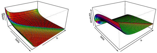
Figure 3. Graphical presentation of the $E\left(X\right)$ (left) and $Var$ (right).

2.4. The MRL and Asymptotic

Within the domains of reliability and survival analysis, the MRL plays a good role as a statistical measure. It quantifies the expected remaining lifetime of a system or component that has survived up to a specific time, making it indispensable in assessing longevity and operational performance across diverse applications from mechanical and electronic systems to biomedical and actuarial sciences. The MRL is instrumental in supporting decision-making processes in engineering, risk management, and reliability design. Mathematically, for a non-negative random variable T with survival function $s\left(t\right)$, the MRL at time t is

$${\mu }_X\left(t\right)=\mathbb{E}[X-t\mid X\ge t]={\displaystyle \frac{1}{s\left(t\right)}}{\int }_t^{\infty }s\left(x\right)dx.$$

The MRL of the proposed distribution is obtained by evaluating the integral above using the corresponding $s\left(t\right).$ Therefore,

$$\begin{array}{cc}\hfill {\mu }_X\left(t\right)& ={\displaystyle \frac{1}{R\left(t\right)}}\sum _{i=0}^{\infty }\sum _{j,k=1}^i{\displaystyle \frac{{(-1)}^{i+j}\left(\genfrac{}{}{0pt}{}{i}{j}\right)\left(\genfrac{}{}{0pt}{}{i}{k}\right)}{i!}}{b}^{i-j}{a}^j{\int }_t^{\infty }{x}^j{e}^{-j\alpha x^{\beta }}dx\hfill \\ \hfill & ={\displaystyle \frac{1}{R\left(t\right)}}\sum _{i=0}^{\infty }\sum _{j,k=1}^i{\displaystyle \frac{{(-1)}^{i+j}\left(\genfrac{}{}{0pt}{}{i}{j}\right)\left(\genfrac{}{}{0pt}{}{i}{k}\right)b^{i-j}{a}^j}{i!}}{\displaystyle \frac{\Gamma (v,\alpha j{t}^{\beta })}{\beta {\left(\alpha j\right)}^v}}.\hfill \end{array}$$

where $v={\displaystyle \frac{j+1}{\beta }}.$

The MRL and FRF are inversely related in the sense that they describe different aspects of the same survival behavior. MRL and FRF are linked mathematically because the MRL can be expressed in terms of the FRF, since $s\left(t\right)=e^{\left[-{\int }_0^{t}h\left(x\right)dx\right]}.$ Moreover, the MRL and FRF $h\left(t\right)$ are related by $h\left(t\right)=[{\mu }_X^{\prime }\left(t\right)+1]/{\mu }_X\left(t\right).$ Clearly, ${\mu }_X^{\prime }\left(t\right)\ge -1.$ The MRL and FRF uniquely determine a distribution, see [20,21]. Additional, the relation discussed in [22] is as follows: increasing MRL ⇒ decreasing FRF and decreasing MRL ⇒ increasing FRF. Further, ref. [23] proved that an upside-down bathtub shape MRL ⇒ bathtub shape FRF. Moreover, ref. [24] discussed that the MRL and FRF have a reciprocal relationship as ${lim}_{t\to \infty }{\mu }_X\left(t\right)={lim}_{t\to \infty }{\displaystyle \frac{1}{h\left(t\right)}}.$ Consequently, we can say that the bathtub shape MRL ⇒ upside-down bathtub shape FRF. One can see [25]. Figure 4 and Figure 5 demonstrate the graphical analysis, highlighting how variations in parameters affect the inverse relationship between these two reliability measures.

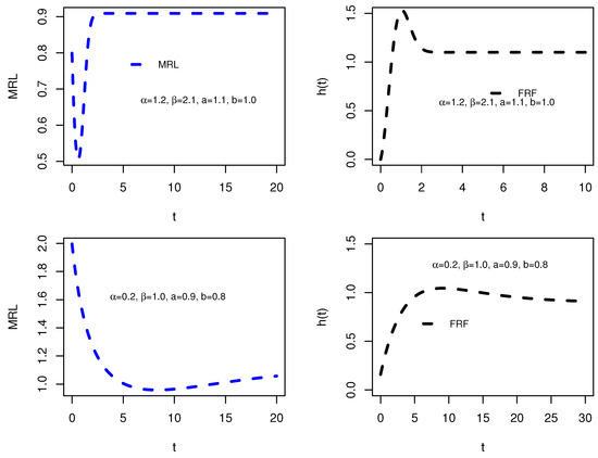
Figure 4. Plots of the reciprocal behavior of the MRL (left) and the corresponding FRF (right) I.

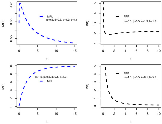
Figure 5. Plots of the reciprocal behavior of the MRL (left) and the corresponding FRF (right) II.

The asymptotic of the MRL is used to assess the long-term reliability of systems, especially in complex engineering systems where it helps in understanding how system reliability evolves over time, particularly in aging or degrading components. In studies of population health, asymptotic MRL provides insights into the average remaining lifetime of individuals in a population after reaching a certain age, aiding in the assessment of life expectancy trends and the impact of public health interventions.

Theorem 2.

The asymptotic of the MRL of the proposed model as $t\to \infty$ is

$${\mu }_X\left(t\right)\sim {\displaystyle \frac{1}{a}}.$$

(12)

Proof. 

The asymptotic of $s\left(x\right)$ in (6) can be obtained:

$$S\left(x\right)=e^{\left(-(ax+b)\right)}{e}^{\left((ax+b)e^{-\alpha x^{\beta }}\right)},$$

Since the linear part grows only linearly in x, while exponential part decays very fast, we have

$$\underset{x\to \infty }{lim}(ax+b)e^{-\alpha x^{\beta }}=0,$$

and

$$\underset{x\to \infty }{lim}{\displaystyle \frac{e^{\left(-(ax+b)(1-e^{-\alpha x^{\beta }})\right)}}{e^{\left(-(ax+b)\right)}}}=e^0=1.$$

Thus,

$$\underset{x\to \infty }{lim}s\left(x\right)\sim e^{-(ax+b)}.$$

Therefore, as $t\to \infty$,

$${\mu }_X\left(t\right)=E(X-t|X>t)={\int }_0^{\infty }{\displaystyle \frac{s(x+t)}{s\left(t\right)}}dx\sim e^{(at+b)}{\int }_0^{\infty }{e}^{-\left(a\right(x+t)+b)}dx={\int }_0^{\infty }{e}^{-ax}dx={\displaystyle \frac{1}{a}}.$$

   □

Figure 6 shows how the asymptotic of the MRL can approximate the true MRL in some cases.

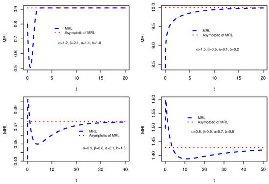
Figure 6. Plots of the MRL and its asymptotic.

2.5. Order Statistics and Asymptotic

In mechanical engineering, order statistics can be applied to study the distribution of material strengths. By analyzing the order statistics of material strength data, engineers can understand the variability and reliability of materials used in construction and manufacturing. The maximum stress that a material can withstand before failure (maximum order statistic) is critical for ensuring safety and performance. Extreme order statistics help in determining the stress limits and safety margins for materials and structures, thereby preventing catastrophic failures (see [26]).

Let $X_1,X_2,\dots ,X_n$, $n\ge 1$, be an ordered sample from the proposed model; the PDF of the $j^{th}-$ order statistics is $f_{j:n}\left(x\right)$, defined by

$$\begin{array}{c}\hfill f_{X_{j:n}}\left(x\right)=\sum _{m=0}^{n-j}{\displaystyle \frac{n!{(-1)}^m}{(j-1)!(n-j-m)!m!}}f\left(x\right)F^{j+m-1}\left(x\right).\end{array}$$

(13)

Therefore, for $F\left(x\right)$ in (3) and $f\left(x\right)$ in (4),

$$\begin{array}{cc}\hfill f_{X_{j:n}}\left(x\right)& =\sum _{m=0}^{n-j}{\displaystyle \frac{n!{(-1)}^m[a(1-e^{-\alpha x^{\beta }})+\alpha \beta (ax+b)x^{\beta -1}{e}^{-\alpha x^{\beta }}]}{(j-1)!(n-j-m)!m!}}\hfill \\ \hfill & \times {\left(1-e^{-(ax+b)(1-e^{-\alpha x^{\beta }})}\right)}^{j+m-1}{e}^{-(ax+b)(1-e^{-\alpha x^{\beta }})}.\hfill \end{array}$$

The asymptotic distributions of the extreme order statistics, specifically the $X_{1:n}$ and $X_{n:n}$ from a sequence $X_1,X_2,X_3,\dots ,X_n$ that follows the proposed model, are derived as detailed in [27].

Theorem 3.

Let $X_1\le \dots \le X_n$ be from the proposed model and let $B_n=(X_{n:n}-a_n)/b_n$; then, $B_n\stackrel{d}{\to }B$ implies that

$$\underset{n\to \infty }{lim}P(B_n\le x)=G\left(x\right)=e^{-e^{-x}},$$

$\vee x\in \Re$ of $G\left(x\right)$, $a_n=q(1-n^{-1})$, and $b_n=E[X-a_n|X>a_n]$ according to Theorem 8.3.4 of [27], where $q(·)$ in (7).

Proof. 

Considering Theorem 8.3.2 of [27], we use the asymptotic of the MRL in (12), and we have

$$\underset{t\to \infty }{lim}{\displaystyle \frac{R(t+xE(X-t|X>t))}{R\left(t\right)}}\sim \underset{t\to \infty }{lim}{\displaystyle \frac{e^{-a(t+\frac{x}{a})}}{e^{-(at+b)}}}\sim e^{-x}.$$

   □

Theorem 4.

Let $X_1\le \dots \le X_n$ be from the proposed model and let $B_n^{\ast }=(X_{1:n}-a_n^{\ast })/b_n^{\ast }$; then, $B_n^{\ast }\stackrel{d}{\to }{B}^{\ast }$ is equivalent to saying

$$\underset{n\to \infty }{lim}P(B_n^{\ast }\le x)=G^{\ast }\left(x\right)=1-e^{-x^{\beta }}.$$

for every point $x\in {\Re }^{+}$ of $G^{\ast }\left(x\right)$ for which $G^{\ast }\left(x\right)$ is continuous. From Theorem 8.3.6 of [27], $a_n^{\ast }=0$ and $b_n^{\ast }=q\left({\displaystyle \frac{1}{n}}\right)$, where $q(·)$ is in (7).

Proof. 

We start with

$$\underset{x\to 0}{lim}F\left(x\right)\sim (ax+b)(1-e^{-\alpha x^{\beta }})\sim \alpha b{x}^{\beta }.$$

By Theorem 8.3.6 of [27], we can show that

$$\underset{t\to 0}{lim}{\displaystyle \frac{F\left(tx\right)}{F\left(t\right)}}\sim \underset{t\to 0}{lim}{\displaystyle \frac{\alpha b{\left(tx\right)}^{\beta }}{\alpha b{t}^{\beta }}}=x^{\beta }.$$

   □

2.6. Model Identifiability

Evaluating the identifiability of a probability model based on its parameters is a crucial step in statistical modeling. It involves assessing whether the observed data provide enough information to uniquely distinguish among different parameter values. A common and effective tool for this purpose is the Kullback–Leibler divergence (KLD), which quantifies the dissimilarity between two models. As noted in [28], the KLD offers a theoretical foundation for investigating parameter identifiability. In this study, we adopt a widely accepted identifiability criterion based on KLD, which is formally stated as follows.

Let $\Pi (\mathit{x},\mathit{\xi })$ denote a statistical model parameterized by $\mathit{\xi }\in {\mathbb{R}}^d$. The parameter $\mathit{\xi }$ is said to be locally (or globally) identifiable if it is the unique solution to the equation $\mathrm{KLD}(\mathit{\xi },\mathit{\zeta })=0$ within an open neighborhood (or the entire space) of $\mathit{\xi }$ in ${\mathbb{R}}^d$. The Kullback–Leibler divergence between the parameter vectors $\mathit{\xi }$ and $\mathit{\zeta }$ is defined as

$$\mathrm{KLD}(\mathit{\xi },\mathit{\zeta })={\mathbb{E}}_{\mathit{\xi }}\left[log\left({\displaystyle \frac{\Pi (\mathit{x},\mathit{\xi })}{\Pi (\mathit{x},\mathit{\zeta })}}\right)\right]=\int \Pi (\mathit{x},\mathit{\xi })log\left({\displaystyle \frac{\Pi (\mathit{x},\mathit{\xi })}{\Pi (\mathit{x},\mathit{\zeta })}}\right)\mathrm{d}\mathit{x}.$$

(14)

It is important to note that $\mathrm{KLD}(\mathit{\xi },\mathit{\zeta })\ge 0$ for all $\mathit{\zeta }$, and equality holds if and only if $\Pi (\mathit{x},\mathit{\xi })=\Pi (\mathit{x},\mathit{\zeta })$ almost everywhere in $\mathit{x}\in {\mathbb{R}}^d$. However, due to the inherent complexity of many probability density functions, deriving a closed-form expression for the KLD in (14) is often analytically intractable. For further theoretical insights and illustrative examples, the reader is referred to [28]. In this work, we numerically evaluate the Kullback–Leibler divergence $\mathrm{KLD}(\mathit{\gamma },\mathit{\delta })$ for the proposed model. Consider two random variables: $X_1\sim f(x;\mathit{\xi })$ and $X_2\sim f(x;\mathit{\zeta })$, where the parameter vectors are given by $\mathit{\xi }={({\alpha }^{\diamond },{\beta }^{\diamond },a^{\diamond },b^{\diamond })}^{\prime }$ and $\mathit{\zeta }={({\alpha }^{♯},{\beta }^{♯},a^{♯},b^{♯})}^{\prime }$. Based on the definition in Equation (14), the KLD between these two parameterizations can be expressed as

$$\begin{array}{cc}\hfill & \mathrm{KLD}(\mathit{\xi },\mathit{\zeta })={\int }_0^{\infty }[a^{\diamond }(1-e^{-{\alpha }^{\diamond }{x}^{{\beta }^{\diamond }}})+{\alpha }^{\diamond }{\beta }^{\diamond }(a^{\diamond }x+b^{\diamond })x^{{\beta }^{\diamond }-1}{e}^{-{\alpha }^{\diamond }{x}^{{\beta }^{\diamond }}}]e^{-(a^{\diamond }x+b^{\diamond })(1-e^{-{\alpha }^{\diamond }{x}^{{\beta }^{\diamond }}})}\hfill \\ \hfill & \times log\left([a^{\diamond }(1-e^{-{\alpha }^{\diamond }{x}^{{\beta }^{\diamond }}})+{\alpha }^{\diamond }{\beta }^{\diamond }(a^{\diamond }x+b^{\diamond })x^{{\beta }^{\diamond }-1}{e}^{-{\alpha }^{\diamond }{x}^{{\beta }^{\diamond }}}]e^{-(a^{\diamond }x+b^{\diamond })(1-e^{-{\alpha }^{\diamond }{x}^{{\beta }^{\diamond }}})}\right)dx\hfill \\ \hfill & -{\int }_0^{\infty }[a^{\diamond }(1-e^{-{\alpha }^{\diamond }{x}^{{\beta }^{\diamond }}})+{\alpha }^{\diamond }{\beta }^{\diamond }(a^{\diamond }x+b^{\diamond })x^{{\beta }^{\diamond }-1}{e}^{-{\alpha }^{\diamond }{x}^{{\beta }^{\diamond }}}]e^{-(a^{\diamond }x+b^{\diamond })(1-e^{-{\alpha }^{\diamond }{x}^{{\beta }^{\diamond }}})}\hfill \\ \hfill & \times log\left([a^{♯}(1-e^{-{\alpha }^{♯}{x}^{{\beta }^{♯}}})+{\alpha }^{♯}{\beta }^{♯}(a^{♯}x+b^{♯})x^{{\beta }^{♯}-1}{e}^{-{\alpha }^{♯}{x}^{{\beta }^{♯}}}]e^{-(a^{♯}x+b^{♯})(1-e^{-{\alpha }^{♯}{x}^{{\beta }^{♯}}})}\right)dx.\hfill \end{array}$$

(15)

Due to the analytical intractability of Equation (15), we employ a numerical integration available in R software. To investigate the identifiability of the model, we consider selected parameter scenarios; here, there is no systematic method of parameter choice because it is not a specific application that requires parameter optimization. Specifically, we fix the parameter vectors $\mathit{\xi }={({\alpha }^{\diamond }=1.5,{\beta }^{\diamond }=0.5,a^{\diamond }=1.2,b^{\diamond }=1.3)}^{\prime }$ and $\mathit{\xi }={({\alpha }^{\diamond }=1.0,{\beta }^{\diamond }=2.5,a^{\diamond }=3.5,b^{\diamond }=2.0)}^{\prime }$ and construct several alternative vectors $\mathit{\zeta }$, considering both the case where $\mathit{\xi }\ne \mathit{\zeta }$ and the case where $\mathit{\xi }=\mathit{\zeta }$. The corresponding KLD values computed for each scenario are summarized in Table 3 and Table 4. The results demonstrate that $\mathrm{KLD}(\mathit{\xi },\mathit{\zeta })>0$ whenever $\mathit{\xi }\ne \mathit{\zeta }$ and that $\mathrm{KLD}(\mathit{\xi },\mathit{\zeta })=0$ holds only when $\mathit{\xi }=\mathit{\zeta }$. These outcomes support the identifiability of the proposed model under the considered cases. Nonetheless, we recognize that these illustrative examples alone do not suffice to establish general claims about the local or global identifiability of the proposed model across its entire parameter space.

Table 3. Kullback–Leibler divergence values based on (15) for identifiability assessment for $\mathit{\xi }={({\alpha }^{\diamond }=1.5, {\beta }^{\diamond }=0.5, a^{\diamond }=1.2, b^{\diamond }=1.3)}^{\prime }$.

Cases	Hypothesis $\mathit{\xi }\ne \mathit{\zeta }$ and $\mathit{\xi }=\mathit{\zeta }$	$\mathit{K}\mathit{L}\mathit{D}(\mathit{\xi },\mathit{\zeta })$	Absolute Error
1	${\alpha }^{\diamond }\ne {\alpha }^{♯}$	$0.4977627$	$5.4\times {10}^{-6}$
2	${\beta }^{\diamond }\ne {\beta }^{♯}$	$3.75224$	$0.00014$
3	$a^{\diamond }\ne a^{♯}$	$0.01682013$	$7.1\times {10}^{-7}$
4	$b^{\diamond }\ne b^{♯}$	$0.09657647$	$5.6\times {10}^{-5}$
5	${\alpha }^{\diamond }\ne {\alpha }^{♯},{\beta }^{\diamond }\ne {\beta }^{♯}$	$0.8761882$	$2\times {10}^{-5}$
6	${\alpha }^{\diamond }\ne {\alpha }^{♯},a^{\diamond }\ne a^{♯}$	$0.03799898$	$3.3\times {10}^{-7}$
7	${\alpha }^{\diamond }\ne {\alpha }^{♯},b^{\diamond }\ne b^{♯}$	$0.4061548$	$0.00012$
8	${\beta }^{\diamond }\ne {\beta }^{♯},a^{\diamond }\ne a^{♯}$	$8.154141$	$2.6\times {10}^{-5}$
9	${\beta }^{\diamond }\ne {\beta }^{♯},b^{\diamond }\ne b^{♯}$	$8.094597$	$2.6\times {10}^{-5}$
10	$a^{\diamond }\ne a^{♯},b^{\diamond }\ne b^{♯}$	$0.8877135$	$1.4\times {10}^{-5}$
11	${\alpha }^{\diamond }\ne {\alpha }^{♯},{\beta }^{\diamond }\ne {\beta }^{♯},a^{\diamond }\ne a^{♯}$	$3.399457$	$0.00024$
12	${\alpha }^{\diamond }\ne {\alpha }^{♯},{\beta }^{\diamond }\ne {\beta }^{♯},b^{\diamond }\ne b^{♯}$	$3.505957$	$2.3\times {10}^{-5}$
13	${\alpha }^{\diamond }\ne {\alpha }^{♯},a^{\diamond }\ne a^{♯},b^{\diamond }\ne b^{♯}$	$0.08959356$	$5.1\times {10}^{-6}$
14	${\beta }^{\diamond }\ne {\beta }^{♯},a^{\diamond }\ne a^{♯},b^{\diamond }\ne b^{♯}$	$0.1240934$	$2.8\times {10}^{-6}$
15	$\mathit{\xi }\ne \mathit{\zeta }$	$0.185077$	$7.5\times {10}^{-6}$
16	$\mathit{\xi }=\mathit{\zeta }$	0	0

Table 4. Kullback–Leibler divergence values based on (15) for identifiability assessment for $\mathit{\xi }={({\alpha }^{\diamond }=1.0, {\beta }^{\diamond }=2.5, a^{\diamond }=3.5, b^{\diamond }=2.0)}^{\prime }$.

Cases	Hypothesis $\mathit{\xi }\ne \mathit{\zeta }$ and $\mathit{\xi }=\mathit{\zeta }$	$\mathit{K}\mathit{L}\mathit{D}(\mathit{\xi },\mathit{\zeta })$	Absolute Error
1	${\alpha }^{\diamond }\ne {\alpha }^{♯}$	$0.02897477$	$1.0\times {10}^{-6}$
2	${\beta }^{\diamond }\ne {\beta }^{♯}$	$0.06974003$	$3.0\times {10}^{-5}$
3	$a^{\diamond }\ne a^{♯}$	$0.1807974$	$9.7\times {10}^{-7}$
4	$b^{\diamond }\ne b^{♯}$	$0.02100667$	$4.6\times {10}^{-7}$
5	${\alpha }^{\diamond }\ne {\alpha }^{♯},{\beta }^{\diamond }\ne {\beta }^{♯}$	$0.1718268$	$3.6\times {10}^{-5}$
6	${\alpha }^{\diamond }\ne {\alpha }^{♯},a^{\diamond }\ne a^{♯}$	$0.01226518$	$2\times {10}^{-6}$
7	${\alpha }^{\diamond }\ne {\alpha }^{♯},b^{\diamond }\ne b^{♯}$	$0.03529691$	$0.00012$
8	${\beta }^{\diamond }\ne {\beta }^{♯},a^{\diamond }\ne a^{♯}$	$0.27438$	$5.6\times {10}^{-5}$
9	${\beta }^{\diamond }\ne {\beta }^{♯},b^{\diamond }\ne b^{♯}$	$0.2577892$	$5.7\times {10}^{-5}$
10	$a^{\diamond }\ne a^{♯},b^{\diamond }\ne b^{♯}$	$0.008167639$	$2.9\times {10}^{-5}$
11	${\alpha }^{\diamond }\ne {\alpha }^{♯},{\beta }^{\diamond }\ne {\beta }^{♯},a^{\diamond }\ne a^{♯}$	$0.02853821$	$7.4\times {10}^{-5}$
12	${\alpha }^{\diamond }\ne {\alpha }^{♯},{\beta }^{\diamond }\ne {\beta }^{♯},b^{\diamond }\ne b^{♯}$	$0.03693935$	$7.0\times {10}^{-5}$
13	${\alpha }^{\diamond }\ne {\alpha }^{♯},a^{\diamond }\ne a^{♯},b^{\diamond }\ne b^{♯}$	$0.01818254$	$7.0\times {10}^{-5}$
14	${\beta }^{\diamond }\ne {\beta }^{♯},a^{\diamond }\ne a^{♯},b^{\diamond }\ne b^{♯}$	$0.2593118$	$5.8\times {10}^{-5}$
15	$\mathit{\xi }\ne \mathit{\zeta }$	$0.2392815$	$4.1\times {10}^{-6}$
16	$\mathit{\xi }=\mathit{\zeta }$	0	0

3. Information Metrics

Entropy, as conceptualized in information theory and various scientific fields, quantifies the uncertainty associated with the occurrence of a particular event based on partial knowledge about the event or system. It is crucial in diverse areas, including reliability and life sciences. In this context, we discuss extropy (Ex), which is quantified as $Ex=-{\displaystyle \frac{1}{2}}{\int }_{-\infty }^{\infty }{f}^2\left(x\right)dx$, and cumulative residual entropy (CRE), quantified as $CRE=-{\int }_{-\infty }^{\infty }s\left(x\right)logs\left(x\right)dx$. To calculate these measures for the proposed model, the following lemma is required.

Lemma 2.

Let X follow the proposed model and let

$$D_{j,k}(c_1,c_2,c_3,c_4)={\int }_0^{\infty }{(ax+b)}^{c_1}{(1-e^{-\alpha x^{\beta }})}^{c_2}{x}^{c_3-1}{e}^{-c_4{x}^{\beta }}dx,$$

Then,

$$D_{j,k}(c_1,c_2,c_3,c_4)=\sum _{j=0}^{c_1}\sum _{k=0}^{c_2}\left(\genfrac{}{}{0pt}{}{c_1}{j}\right)\left(\genfrac{}{}{0pt}{}{c_2}{k}\right){(-1)}^k{a}^j{b}^{c_1-j}\left({\displaystyle \frac{\gamma (z_1,(\alpha k+c_4)u^{\beta })+\Gamma (z_1,(\alpha k+c_4)u^{\beta })}{\beta {(\alpha k+c_4)}^{z_1}}}\right),$$

for some $u>0$, where $z_1={\displaystyle \frac{c_3+j}{\beta }}.$

Proof. 

It follows a similar way to the computation of (10).    □

• Recently, ref. [29] developed a new measure of randomness of a random variable called Ex, also referred as a complement dual of Shannon entropy (for recent studies see [30,31]). The Ex of X that follows the proposed model is as follows:

  $$\begin{array}{cc}\hfill Ex=& \sum _{i=0}^{\infty }{\displaystyle \frac{{(-1)}^{i+1}{a}^2{2}^{i-1}}{i!}}{\int }_0^{\infty }{(ax+b)}^i{(1-e^{-\alpha x^{\beta }})}^{i+2}dx\hfill \\ \hfill & +a\alpha \beta \sum _{i=1}^{\infty }{\displaystyle \frac{{(-1)}^{i+1}{2}^i}{i!}}{\int }_0^{\infty }{(ax+b)}^{i+1}{(1-e^{-\alpha x^{\beta }})}^{i+1}{x}^{\beta -1}{e}^{-\alpha x^{\beta }}dx\hfill \\ \hfill & +a^2{\beta }^2\sum _{i=1}^{\infty }{\displaystyle \frac{{(-1)}^{i+1}{2}^{i-1}}{i!}}{\int }_0^{\infty }{(ax+b)}^{i+1}{(1-e^{-\alpha x^{\beta }})}^i{x}^{2(\beta -1)}{e}^{-2\alpha x^{\beta }}dx.\hfill \end{array}$$

  Therefore,

  $$\begin{array}{cc}\hfill Ex=& \sum _{i=0}^{\infty }{\displaystyle \frac{{(-1)}^{i+1}{a}^2{2}^{i-1}}{i!}}{D}_{j,k}(i,i+2,1,0)+a\alpha \beta \sum _{i=1}^{\infty }{\displaystyle \frac{{(-1)}^{i+1}{2}^i}{i!}}{D}_{j,k}(i+1,i+1,\beta ,\alpha )\hfill \\ \hfill & +a^2{\beta }^2\sum _{i=1}^{\infty }{\displaystyle \frac{{(-1)}^{i+1}{2}^{i-1}}{i!}}{D}_{j,k}(i+1,i,2\beta -1,2\alpha ).\hfill \end{array}$$

  where $D_{j,k}(·,·,·,·)$ is given by Lemma 2.
• The $CRE$ of X that follows the proposed model is as follows:

  $$\begin{array}{cc}\hfill CRE=& {\int }_0^{\infty }(ax+b)(1-e^{-\alpha x^{\beta }})e^{-(ax+b)(1-e^{-\alpha x^{\beta }})}dx\hfill \\ \hfill & =\sum _{i=0}^{\infty }{\displaystyle \frac{{(-1)}^i}{i!}}{\int }_0^{\infty }{(ax+b)}^{i+1}{(1-e^{-\alpha x^{\beta }})}^{i+1}dx\hfill \\ \hfill & =\sum _{i=0}^{\infty }{\displaystyle \frac{{(-1)}^i}{i!}}{D}_{j,k}(i+1,i+1,1,0).\hfill \end{array}$$

  where $D_{j,k}(·,·,·,·)$ is given by the Lemma 2.

Table 5 presents numerical values of Ex and CRE for selected parameter values. For Ex, the results are consistently negative but increase toward zero as $\beta$ and a grow, indicating a gradual reduction in magnitude and suggesting less uncertainty in the distribution. Similarly, larger values of $\alpha$ shift Ex closer to zero. For CRE, the values are positive and decrease monotonically as the parameters increase. In particular, CRE starts at relatively high values for small parameter settings and declines steadily to very small values (at $\alpha =2.0, \beta =10.0$). Both measures reflect a reduction in the dispersion and concentration of the distribution as parameter values increase.

Table 5. Numerical values of extropy and cumulative residual entropy for some parameter values.

$\mathit{\alpha }$	$\mathit{\beta }$	a	b	$\mathit{E}\mathit{x}$	$\mathit{\alpha }$	$\mathit{\beta }$	a	b	$\mathit{E}\mathit{x}$
0.5	1.0	1.0	0.5	−0.17712	1.5	6.0	6.0	1.5	−0.08037
	1.44	1.44		−0.16536		6.44	6.44		−0.07565
	1.89	1.89		−0.15421		6.89	6.89		−0.07144
	2.33	2.33		−0.14288		7.33	7.33		−0.6765
	2.78	2.78		−0.13206		7.78	7.78		−0.06423
	3.22	3.22		−0.12210		8.22	8.22		−0.06113
	3.67	3.67		−0.011312		8.67	8.67		−0.05829
	4.11	4.11		−0.105078		9.11	9.11		−0.05571
	4.56	4.56		−0.09791		9.56	9.56		−0.05333
	5.0	5.0		−0.09152		10.0	10.0		−0.05114
$\mathit{\alpha }$	$\mathit{\beta }$	a	b	$\mathit{C}\mathit{R}\mathit{E}$	$\mathit{\alpha }$	$\mathit{\beta }$	a	b	$\mathit{C}\mathit{R}\mathit{E}$
0.2	0.5	0.5	0.2	3.57638	2.0	5.5	5.5	2.0	0.11270
	1.0	1.0		1.31818		6.0	6.0		0.10519
	1.5	1.5		0.76105		6.5	6.5		0.09878
	2.0	2.0		0.52448		7.0	7.0		0.09321
	2.5	2.5		0.39678		7.5	7.5		0.08832
	3.0	3.0		0.31794		8.0	8.0		0.08399
	3.5	3.5		0.26493		8.5	8.5		0.08009
	4.0	4.0		0.22709		9.0	9.0		0.07659
	4.5	4.5		0.19886		9.5	9.5		0.07340
	5.0	5.0		0.17705		10.0	10.0		0.07049

4. Reliability Parameter ($R_{ss}$)

In the field of reliability studies, the stress–strength reliability parameter, commonly denoted by $R_{ss}=P(X<Y)$, serves as a key probabilistic measure for evaluating system robustness. It quantifies the probability that a component’s strength Y exceeds the imposed stress X, where failure is deemed to occur when the applied stress surpasses the available strength. Although $R_{ss}$ is traditionally employed in reliability engineering, its applicability spans a range of disciplines, including biomedical science, economics, and other applied fields, as noted in [32]. The analysis of this parameter often assumes that X and Y are independent random variables and has been carried out under numerous statistical distributions. Notable contributions include investigations based on the generalized exponential distribution [33], inverse Pareto distribution [34], Poisson half-logistic distribution [35], and the two-parameter exponential distribution [36], among others. These studies illustrate the versatility of the stress–strength model in diverse reliability contexts.

We now proceed to define a stress–strength reliability measure within the framework of the proposed model. Consider two independent random variables: X, which follows a probability density function $f_1(x;{\alpha }_1,\beta ,a,b)$, and Y, characterized by a cumulative distribution function $F_2(y;{\alpha }_2,\beta ,a,b)$. Under this setup, the reliability parameter is derived in a computational way outlined in Equation (11) and Lemma 2.

$$\begin{array}{cc}\hfill R_{ss}& ={\int }_0^{\infty }{f}_1\left(x\right)F_2\left(x\right)dx\hfill \\ \hfill & ={\int }_0^{\infty }\left[a(1-e^{-{\alpha }_1{x}^{\beta }})+{\alpha }_1\beta (ax+b)x^{\beta -1}{e}^{-{\alpha }_1{x}^{\beta }}\right]\hfill \\ \hfill & \times \left(1-e^{-(ax+b)(1-e^{-{\alpha }_2{x}^{\beta }})}\right)e^{-(ax+b)(1-e^{-{\alpha }_1{x}^{\beta }})}dx\hfill \\ \hfill & =1-{\int }_0^{\infty }\left[a(1-e^{-{\alpha }_1{x}^{\beta }})+{\alpha }_1\beta (ax+b)x^{\beta -1}{e}^{-{\alpha }_1{x}^{\beta }}\right]\hfill \\ \hfill & \times e^{-(ax+b)(1-e^{-{\alpha }_2{x}^{\beta }})}{e}^{-(ax+b)(1-e^{-{\alpha }_1{x}^{\beta }})}dx.\hfill \end{array}$$

(16)

By applying exponential series expansion and then binomial expansion on $(1-e^{-{\alpha }_2{x}^{\beta }}),$ we get

$$e^{-(ax+b)(1-e^{-{\alpha }_2{x}^{\beta }})}{e}^{-(ax+b)(1-e^{-{\alpha }_1{x}^{\beta }})}=\sum _{i,l=0}^{\infty }\sum _{m=0}^l{\displaystyle \frac{{(-1)}^{i+l+m}\left(\genfrac{}{}{0pt}{}{l}{m}\right)}{i!l!}}{(ax+b)}^{i+l}{(1-e^{-{\alpha }_1{x}^{\beta }})}^i{e}^{-{\alpha }_{2}m{x}^{\beta }}.$$

Therefore, (16) becomes

$$\begin{array}{cc}\hfill R_{ss}& =1-a\sum _{i,l=0}^{\infty }\sum _{m=0}^l{\displaystyle \frac{{(-1)}^{i+l+m}\left(\genfrac{}{}{0pt}{}{l}{m}\right)}{i!l!}}{\int }_0^{\infty }{(ax+b)}^{i+l}{(1-e^{-{\alpha }_1{x}^{\beta }})}^{i+1}{e}^{-{\alpha }_{2}m{x}^{\beta }}dx.\hfill \\ \hfill & -{\alpha }_1\beta \sum _{i,l=0}^{\infty }\sum _{m=0}^l{\displaystyle \frac{{(-1)}^{i+l+m}\left(\genfrac{}{}{0pt}{}{l}{m}\right)}{i!l!}}{\int }_0^{\infty }{(ax+b)}^{i+l+1}{(1-e^{-{\alpha }_1{x}^{\beta }})}^i{x}^{\beta -1}{e}^{-({\alpha }_1+{\alpha }_{2}m)x^{\beta }}dx.\hfill \end{array}$$

(17)

The integrals in (17) can be obtained by considering Lemma 2. Thus,

$$\begin{array}{cc}\hfill R_{ss}& =1-a\sum _{i,l=0}^{\infty }\sum _{m=0}^l{\displaystyle \frac{{(-1)}^{i+l+m}\left(\genfrac{}{}{0pt}{}{l}{m}\right)}{i!l!}}{D}_{j,k}(i+l,i+1,0,{\alpha }_{2}m)\hfill \\ \hfill & -{\alpha }_1\beta \sum _{i,l=0}^{\infty }\sum _{m=0}^l{\displaystyle \frac{{(-1)}^{i+l+m}\left(\genfrac{}{}{0pt}{}{l}{m}\right)}{i!l!}}{D}_{j,k}(i+l+1,i,\beta ,{\alpha }_1+{\alpha }_{2}m),\hfill \end{array}$$

where $D_{j,k}(.,.,.,.)$ is defined in Lemma 2.

5. Estimation

The MLE is considered for parameter estimation and facilitates comparative model evaluation. We restrict attention to the MLE due to its desirable large-sample properties and tractability. Let $x_1,x_2,\dots ,x_n$ be a random sample of size n from the derived model. Let $\Theta ={(\alpha ,\beta ,a,b)}^{\top }$ and let the MLE of $\Theta$ be $\widehat{\Theta }={(\widehat{\alpha },\widehat{\beta },\widehat{a},\widehat{b})}^{\top }$. The log-likelihood function is as follows:

$$L(\Theta )=\sum _{i=1}^{n}logf(x_i;\Theta ),$$

where $f(x_i;\Theta )$ denotes the PDF of the proposed model evaluated at $x_i$. Due to the potential complexity of the likelihood surface, numerical optimization techniques are typically required to compute the MLEs.

$$L(\Theta )=\sum _{i=1}^{n}log[a(1-e^{-\alpha x_i^{\beta }})+\alpha \beta (a{x}_i+b)x_i^{\beta -1}{e}^{-\alpha x_i^{\beta }}]-\sum _{i=1}^n(a{x}_i+b)(1-e^{-\alpha x_i^{\beta }}),$$

(18)

Alternatively, the estimation of $\Theta$ can be carried out by maximizing the nonlinear system of equations presented in Equations (19)–(21). These equations are inherently nonlinear and do not permit analytical solutions. Therefore, iterative numerical procedures must be employed. One practical approach is to apply optimization routines available in statistical computing software, such as the maxLikpackage in R, which implements robust algorithms for solving unconstrained nonlinear maximization problems [37].

$$\begin{array}{cc}\hfill {\displaystyle \frac{\partial L}{\partial a}}& =\sum _{i=1}^n{\displaystyle \frac{[(1-e^{-\alpha x_i^{\beta }})+\alpha \beta k_2\left(x_i\right)]}{k_1\left(x_i\right)}}-\sum _{i=1}^n{x}_i(1-e^{-\alpha x_i^{\beta }}),\hfill \end{array}$$

(19)

$$\begin{array}{cc}\hfill {\displaystyle \frac{\partial L}{\partial b}}& =\sum _{i=1}^n{\displaystyle \frac{\alpha \beta k_3\left(x_i\right)}{k_1\left(x_i\right)}}-\sum _{i=1}^n(1-e^{-\alpha x_i^{\beta }}),\hfill \end{array}$$

(20)

$$\begin{array}{cc}\hfill {\displaystyle \frac{\partial L}{\partial \alpha }}& =\sum _{i=1}^n{\displaystyle \frac{a{k}_2\left(x_i\right)+\beta [1-\alpha x_i^{\beta }](a{x}_i+b)k_3\left(x_i\right)}{k_1\left(x_i\right)}}-\sum _{i=1}^n(a{x}_i+b)k_2\left(x_i\right),\hfill \\ \hfill {\displaystyle \frac{\partial L}{\partial \beta }}& =\sum _{i=1}^n{\displaystyle \frac{a\alpha k_2\left(x_i\right)log{x}_i+\alpha (a{x}_i+b)k_3\left(x_i\right)[1+\beta log{x}_i-\alpha \beta x_i^{\beta }log{x}_i]}{k_1\left(x_i\right)}}\hfill \end{array}$$

(21)

$$\begin{array}{cc}\hfill & -\alpha \sum _{i=1}^n(a{x}_i+b)k_2\left(x_i\right)log{x}_i.\hfill \end{array}$$

(22)

where $k_1\left(x_i\right)=a(1-e^{-\alpha x_i^{\beta }})+\alpha \beta (a{x}_i+b)x_i^{\beta -1}{e}^{-\alpha x_i^{\beta }}$, $k_2\left(x_i\right)=x_i^{\beta }{e}^{-\alpha x_i^{\beta }},$ and $k_3\left(x_i\right)=x_i^{\beta -1}{e}^{-\alpha x_i^{\beta }}.$ Under the standard conditions, the asymptotic of the MLE $\widehat{\Theta }$ is approximated by $N_4(0,{\widehat{J}}^{-1})$, where $\widehat{J}$ denotes the observed Fisher information matrix. The matrix elements of J are given by

$$J=\left[{\displaystyle \frac{{\partial }^{2}L(\Theta )}{\partial \Theta \partial {\Theta }^T}}\right].$$

Let ${\Theta }_r$ denote the $r^{\mathrm{th}}$ component of the parameter vector $\Theta$ for $r=1,\dots ,4$. Then, a $100(1-ϵ)\%$ asymptotic confidence interval for ${\Theta }_r$ is given by

$${\mathrm{ACI}}_r=\left({\Theta }_r\pm z_{ϵ/2}\sqrt{{\widehat{J}}_{rr}^{-1}}\right),$$

where ${\widehat{J}}_{rr}^{-1}$ is the $(r,r)$-th diagonal element of the inverse Fisher information matrix ${\widehat{J}}^{-1}$ and $z_{ϵ/2}$ denotes the upper $(ϵ/2)$-quantile of the standard normal distribution. The diagonal element of the inverse Fisher information matrix can be obtained numerically using R-software by a hessian function in the package ’numDeriv’ [38]. The elements of $\widehat{J}$ are given in Appendix A.

Simulation Results

As described in Section 2.2, random samples of varying sizes ($n=50,100,150,200,250,300$) are generated from the proposed model using pre-specified parameter values. This process is repeated $N=1000$ times for each sample size. For each simulated dataset, the MLEs of the parameters are computed. Subsequently, we assess the estimators’ performance by calculating the bias and mean squared error (MSE) for each parameter across the replications. The simulation results in Table 6, also shown graphically in Figure 7, Figure 8 and Figure 9, demonstrate, as expected, that the accuracy of the parameter estimates improves as the sample size n increases. This trend is consistent across all parameter configurations, with both the MSE and absolute bias decreasing steadily with larger samples. For small sample sizes ($n=50$), parameter estimates exhibit moderate bias and variability, especially under more extreme parameter settings $\alpha =5.0$ and $b=7.0$. However, as n goes to 300, the estimates converge closely to their true values with minimal bias and reduced MSE, indicating strong consistency. In scenarios with moderate parameters, $\alpha =1.0$, $\beta =1.5$, $a=0.6$, and $b=1.2$, the model performs robustly even at smaller n, producing near-unbiased estimates. Similarly, across all cases, the parameter b, which often influences the tail behavior of the distribution, shows increasingly stable estimates as n increases. The observed trend demonstrates that larger sample sizes lead to more accurate estimates, thereby enhancing the overall precision and reliability of the estimation procedure.

Table 6. Simulation results: Average estimate (top), MSE (middle), and bias (in parentheses).

n	$\mathit{\alpha }=0.5$	$\mathit{\beta }=0.5$	$\mathit{a}=0.5$	$\mathit{b}=0.5$	$\mathit{\alpha }=1.0$	$\mathit{\beta }=0.6$	$\mathit{a}=3.0$	$\mathit{b}=4.5$
50	0.5234	0.4871	0.5123	0.5345	1.0041	0.6305	3.0587	4.4717
	0.0256	0.0228	0.0267	0.0284	1.8799	1.4734	1.5409	0.7059
	(0.0234)	(−0.0129)	(0.0123)	(0.0345)	(0.5041)	(0.1305)	(0.5587)	(1.9717)
100	0.5098	0.4932	0.5087	0.5124	0.7448	0.4757	2.8868	3.9000
	0.0156	0.0173	0.0138	0.0142	0.5576	0.9167	0.5860	0.2113
	(0.0098)	(−0.0068)	(0.0087)	(0.0124)	(0.2448)	(−0.0243)	(0.3868)	(1.4000)
150	0.5023	0.4987	0.5034	0.5041	0.8114	0.8547	3.0717	2.3512
	0.0112	0.0109	0.0126	0.0119	0.3197	0.4460	0.6100	0.1987
	(0.0023)	(−0.0013)	(0.0034)	(0.0041)	(−0.0886)	(0.3547)	(0.5717)	(−0.1488)
200	0.4989	0.5012	0.4978	0.5007	0.6462	0.5750	2.7271	3.3909
	0.0087	0.0091	0.0083	0.0085	0.3022	0.4133	0.3134	0.1524
	(−0.0011)	(0.0012)	(−0.0022)	(0.0007)	(0.1462)	(0.0750)	(0.2271)	(0.8909)
250	0.4956	0.4993	0.4967	0.4981	0.6186	0.5275	2.7258	3.2917
	0.0072	0.0069	0.0074	0.0076	0.2367	0.0523	0.2606	0.1078
	(−0.0044)	(−0.0007)	(−0.0033)	(−0.0019)	(0.1186)	(0.0275)	(0.2258)	(0.7917)
300	0.4923	0.4968	0.4945	0.4959	0.5926	0.5007	2.6963	4.1725
	0.0059	0.0062	0.0061	0.0063	0.1802	0.0375	0.2036	0.1016
	(−0.0077)	(−0.0032)	(−0.0055)	(−0.0041)	(0.0926)	(0.0007)	(0.1963)	(0.6725)
n	$\mathit{\alpha }=1.0$	$\mathit{\beta }=1.5$	$\mathit{a}=0.6$	$\mathit{b}=1.2$	$\mathit{\alpha }=1.5$	$\mathit{\beta }=1.0$	$\mathit{a}=1.3$	$\mathit{b}=1.0$
50	1.0235	1.4786	0.6223	1.2445	1.5214	1.0193	1.3225	1.0214
	0.7521	0.9032	0.8041	0.6254	1.1012	0.9024	1.0034	0.9025
	(0.0235)	(−0.0214)	(0.0223)	(0.0445)	(0.0214)	(0.0193)	(0.0225)	(0.0214)
100	1.0126	1.3872	0.6125	1.0103	1.5115	1.0114	1.2112	1.1116
	0.5553	0.6025	0.5034	0.5231	0.8023	0.7534	0.7031	0.7532
	(0.1126)	(−0.0128)	(0.1125)	(0.1103)	(0.0115)	(0.0114)	(0.0112)	(0.0116)
150	1.1057	1.4933	0.5056	1.3054	1.5062	1.1053	1.3065	1.1054
	0.4056	0.5127	0.3532	0.4738	0.5524	0.5023	0.5521	0.5026
	(0.0157)	(−0.0267)	(0.0156)	(0.0154)	(0.0062)	(0.0053)	(0.0065)	(0.0054)
200	1.1029	1.2984	0.5028	1.1026	1.5024	1.0022	1.3026	1.0023
	0.3054	0.3121	0.3023	0.3214	0.4021	0.3524	0.4032	0.3521
	(0.0229)	(−0.0116)	(0.0128)	(0.0126)	(0.0024)	(0.0022)	(0.0026)	(0.0023)
250	1.0114	1.11995	0.5013	1.2015	1.5013	1.0013	1.3015	1.0014
	0.2553	0.2824	0.2521	0.2732	0.3023	0.2825	0.3024	0.2826
	(0.0014)	(−0.0005)	(0.0013)	(0.0015)	(0.0013)	(0.0013)	(0.0015)	(0.0014)
300	1.0006	1.4997	0.6007	1.2008	1.5007	1.0006	1.3007	1.0005
	0.2052	0.2235	0.2031	0.2256	0.2524	0.2226	0.2523	0.2225
	(0.0006)	(−0.0003)	(0.0007)	(0.0008)	(0.0007)	(0.0006)	(0.0007)	(0.0005)
n	$\mathit{\alpha }=5.0$	$\mathit{\beta }=2.5$	$\mathit{a}=1.8$	$\mathit{b}=7.0$	$\mathit{\alpha }=2.5$	$\mathit{\beta }=5.0$	$\mathit{a}=1.0$	$\mathit{b}=3.5$
50	5.0439	2.1222	1.8431	7.9390	2.6631	4.3459	1.0189	3.4711
	0.6380	0.9950	1.9158	0.6475	0.4360	0.9304	0.4111	0.9198
	(0.1439)	(0.9222)	(−0.1569)	(0.4390)	(0.5631)	(0.1459)	(0.1189)	(1.4711)
100	4.4745	2.5562	2.1583	5.6715	2.4877	4.8298	0.9321	3.0172
	0.3692	0.3291	0.9994	0.2498	0.3838	0.8352	0.2062	0.8799
	(0.5745)	(0.3562)	(0.1583)	(0.1715)	(0.3877)	(0.6298)	(0.0321)	(1.0172)
150	5.8920	2.6733	2.1393	7.9688	2.5122	4.8183	0.8880	3.2168
	0.3436	0.3103	0.4978	0.2335	0.2975	0.6764	0.1382	0.5420
	(−0.0080)	(0.4733)	(0.7393)	(0.4688)	(0.4122)	(0.6183)	(−0.0120)	(1.2168)
200	4.9262	1.9153	1.6168	7.6706	2.5469	4.9563	0.8667	3.0654
	0.2076	0.2388	0.3284	0.2178	0.1664	0.3140	0.1154	0.5400
	(0.0262)	(−0.2847)	(−0.3832)	(0.1706)	(0.4469)	(0.7563)	(−0.0333)	(1.0654)
250	4.5965	2.3202	1.6490	6.6485	2.6273	5.3207	0.8452	2.8937
	0.1905	0.1464	0.3166	0.1310	0.0863	0.3051	0.1010	0.3752
	(0.6965)	(−0.2798)	(−0.3510)	(0.1485)	(0.5273)	(0.1207)	(−0.0548)	(0.8937)
300	4.4294	2.3751	1.7087	5.9705	2.5239	5.0342	0.8383	2.7928
	0.0317	0.1006	0.1110	0.1134	0.0151	0.0517	0.0869	0.3173
	(0.5294)	(−0.1249)	(−0.2913)	(0.4705)	(0.4239)	(0.8342)	(−0.0617)	(0.7928)

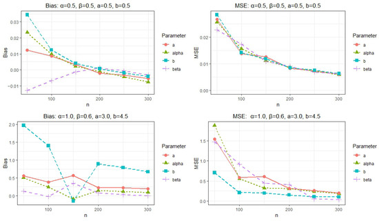
Figure 7. Plots of the simulation results: Bias (left) and MSE (right)-I.

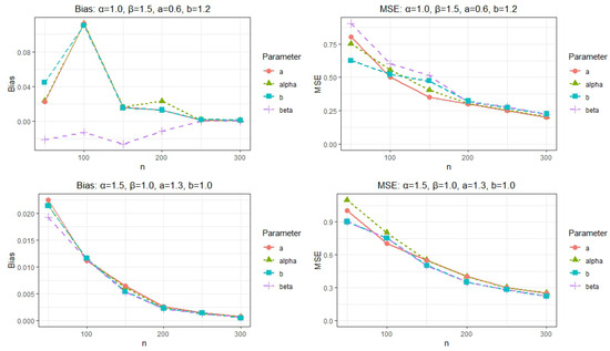
Figure 8. Plots of the simulation results: Bias (left) and MSE (right)-II.

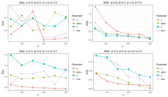
Figure 9. Plots of the simulation results: Bias (left) and MSE (right)-III.

6. Application

In this section, we illustrate the efficacy of the proposed distribution by applying it to real datasets and comparing its performance against various existing distributions. We determined the parameters for each competing model using MLE. The models were then assessed based on different information criteria, such as the Akaike Information Criterion (AIC), Bayesian Information Criterion (BIC), Consistent Akaike Information Criterion (CAIC), and Hannan–Quinn Information Criterion (HQC). Additionally, we evaluated the goodness of fit for each model using statistics like the Kolmogorov–Smirnov (KS), Anderson–Darling (A), and Cramer–von Mises (W) tests. Different model selection and goodness-of-fit criteria serve complementary purposes. Information-based measures such as the AIC, BIC, and CAIC balance model fit against complexity, but they differ in the severity of their penalty terms. The BIC, derived from Bayesian principles, imposes a stronger penalty on additional parameters, often favoring more parsimonious models even if they provide a moderate fit to the data. In contrast, the AIC emphasizes predictive accuracy and may prefer more flexible models. Goodness-of-fit measures such as KS, AD, and CVM, however, evaluate how well the fitted distribution captures the empirical data without considering model parsimony. Therefore, discrepancies among these measures are expected, particularly when the candidate models differ in dimensionality; therefore, for more accuracy, all tests are considered to obtained the best model for the data. The comparison of goodness of fit includes several Weibull-based distributions, with the survival functions detailed in Table 7.

Table 7. Survival function of the alternative models; $x,\alpha ,\beta ,\lambda ,\gamma >0$.

Distribution	s(x)
Modified Weibull (MW) [39]	$exp(-\alpha x^{\beta }{e}^{\lambda x})$
Flexible Weibull (FW) [40]	$exp(-e^{\alpha x-(\beta /x)})$
Exponentiated Weibull (EW) [5]	$1-{(1-e^{-\alpha x^{\beta }})}^{\lambda }$
Additive Weibull (AddW) [41]	$e^{-\alpha x^{\beta }-\lambda x^{\gamma }}$
Modified Weibull extension (MWE) [42]	$exp\left(\alpha \lambda (1-e^{{(x/\alpha )}^{\beta }})\right)$
Exponentiated sine Weibull (ESW) [43]	${sin}^{\alpha }\left({\displaystyle \frac{\pi }{2}}[1-e^{-\alpha x^{\beta }}]\right)$
Extended cosine Weibull (ESW) [44]	$1-{\left(1-cos\left({\displaystyle \frac{\pi }{2}}{e}^{-\alpha x^{\beta }}\right)\right)}^{\lambda }$
Generalized inverse Weibull (GIW) [45]	$1-exp(-\gamma {(\alpha /x)}^{\beta })$
Generalized generalized inverse Weibull (GGIW) [46]	$1-{(1-exp(-\gamma {(\lambda /x)}^{\beta }))}^{\alpha }$

6.1. Dataset I

The dataset consists of the failure times (in weeks) of 50 items, provided by [2]. The findings demonstrate that the proposed distribution provides a markedly better fit than the competing models, as shown by illustrating the ranking results in Figure 10, where it consistently secures the top position, outperforming the alternatives in six out of the seven evaluated statistical criteria. The analysis based on the MLE and confidence interval for the eleven candidate models is summarized in Table 8, and the information matrix of the proposed model is given below. Table 9 highlights that the proposed distribution offers the best overall performance compared to its competitors. Specifically, it attains the highest log-likelihood value ($L=-147.52$) and the smallest values of AIC (303.03), CAIC (303.92), and second-rank BIC (310.68), reflecting its superior balance between goodness of fit and model parsimony. In terms of goodness-of-fit statistics, the proposed model also yields the lowest $A=0.2364$ and $W=0.0389$ values, demonstrating close agreement with the empirical distribution. Furthermore, the KS statistic is minimized at $KS=0.0770$ with the highest associated p-value $\left(0.9060\right)$, providing strong evidence of model adequacy. In general, the proposed model ranked first among all the competing models. Secondly, among competing models, the ESW, AddW, and EW distributions show moderate performance, with reasonably small values of AIC, BIC, and CAIC (around 306 to 308) and acceptable KS values (0.0913 to 0.0965 with p-values between 0.70 and 0.80). However, they remain consistently inferior to the proposed distribution. The W and MWE distributions also provide some fits but fail to surpass the proposed model in likelihood or fit statistics. By contrast, the FW and GIW models exhibit the weakest performance overall. For example, FW yields the lowest log-likelihood ($L=-176.85$) and the largest AIC (357.70) and BIC (361.53), while GIW presents similarly poor results ($L=-168.64$, AIC = 343.28). Both models also record very large A, W, and KS statistics (e.g., FW with $A=3.5194$, $W=0.6649$, and $KS=0.4078$), with extremely low p-values, indicating their inadequacy in capturing the distributional features of the data. The GGIW distribution also fails, with an inflated KS statistic ($KS=0.9983$) and essentially zero p-value. Finally, in support of our results, Figure 11 displays a precise alignment with the empirical data through the fitted survival functions and MRL. Figure 12 further supports our results by showing a box plot and quantile–quantile (QQ) plot, which confirm the proposed model’s compatibility with the observed data.

$$J^{-1}=\left[\begin{array}{cccc}1.15368550& -0.20445018& -0.00212985& 0.01974882\\ -0.20445018& 0.01507867& -0.00062193& 0.00650080\\ -0.00212985& -0.00062193& 0.00030785& -0.00015309\\ 0.01974882& 0.00650080& -0.00015309& 0.00454953\end{array}\right].$$

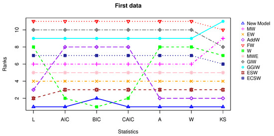
Figure 10. Line plot for ranking assessment based on the statistics for the first dataset.

Table 8. MLEs for first dataset.

Distribution	$\mathit{\alpha }$	$\mathit{\beta }$	$\mathit{\lambda }$	$\mathit{\gamma }$	a	b
New model	4.1459 (0.1030)	0.6318 (0.1283)	-	-	0.1142 (0.0175)	0.1205 (0.0614)
	(2.0408, 6.2512)	(0.3647, 0.8461)	-	-	(0.0786, 0.1474)	(0.0065, 0.2709)
MW	0.2200 (0.0580)	0.7332 (0.13022)	0.0075 (0.0111)	-	-	-
	(0.1063, 0.3338)	(0.4779, 0.9885)	(0.00, 0.0291)	-	-	-
EW	0.0688 (0.0987)	1.1007 (0.3904)	0.5984 (0.3176)	-	-	-
	(0.00, 0.2622)	(0.3355, 1.8659)	(0.00, 1.2209)	-	-	-
AddW	0.0312 (0.1201)	1.2177 (0.3130)	0.6080 (0.0164)	0.18683 (0.1150)	-	-
	(0.00, 0.1996)	(0.1084, 2.3261)	(0.1118, 1.1035)	(0.00, 0.4075)	-	-
FW	0.0458 (0.0046)	0.1417 (0.0384)	-	-	-	-
	(0.0369, 0.0548)	(0.0662. 0.2172)	-	-	-	-
W	0.2114 (0.0555)	0.8006 (0.0908)	-	-	-	-
	(0.1025, 0.3202)	(0.6227, 0.9786)	-	-	-	-
MWE	56.6358 (5.9758)	0.7073 (0.0897)	0.0664 (0.0143)	-	-	-
	(44.9231, 68.3486)	(0.5313, 0.8833)	(0.0384, 0.0943)	-	-	-
GIW	1.1617 (11.413)	0.4790 (0.0454)	1.0476 (4.9291)	-	-	-
	(0.00, 23.5316)	(0.3901, 0.5680)	(0.00, 10.7089)	-	-	-
GGIW	437.5553 (6.4044)	0.1161 (0.0121)	3.0312 (3.0516)	6.61447 (0.8075)	-	-
	(425.003, 450.107)	(0.0923, 0.1398)	(0.00, 9.0123)	(5.0319, 8.1971)	-	-
ESW	0.6579 (0.3302)	0.9915 (0.3358)	0.0553 (0.0675)	-	-	-
	(0.0108, 1.3051)	(0.3333, 1.6496)	(0.00, 0.1875)	-	-	-
ECSW	1.3286 (2.2357)	0.7641 (0.0879)	0.0983 (0.1594)	-	-	-
	(0.00, 5.7106)	(0.5917, 0.9366)	(0.00, 0.4108)	-	-	-

Table 9. L, AIC, BIC, CAIC, A, W, KS (p-value), and rank as superscript for first dataset.

Distribution	L	$\mathit{A}\mathit{I}\mathit{C}$	$\mathit{B}\mathit{I}\mathit{C}$	$\mathit{C}\mathit{A}\mathit{I}\mathit{C}$	A	W	$\mathit{K}\mathit{S}\left(\mathit{p}\mathit{v}\right)$
New Model	−147.52 1	303.03 1	310.68 2	303.92 1	0.2364 1	0.0389 1	0.0770 1 (0.9060)
MW	−150.44 6	306.88 6	312.62 6	307.40 6	0.3562 6	0.0712 6	0.3562 9 (0.6141)
EW	−150.26 4	306.52 4	312.25 4	307.04 4	0.2997 4	0.0593 4	0.0965 4 (0.7038)
AddW	−150.22 3	308.44 8	316.08 8	311.35 8	0.2812 2	0.0545 2	0.0913 2 (0.7986)
FW	−176.85 11	357.70 11	361.53 11	357.96 11	3.5194 11	0.6649 11	0.4078 10 (4.9$\times {10}^{-8}$)
W	−150.67 8	305.35 2	309.18 1	305.61 2	0.4202 8	0.0847 8	0.1119 7 (0.5223)
MWE	−150.37 5	306.74 5	312.48 5	307.26 5	0.3362 5	0.0670 5	0.1023 5 (0.6348)
GIW	−168.64 10	343.28 10	349.01 10	343.80 10	3.2618 10	0.6036 10	0.1993 8 (0.0323)
GGIW	−153.14 9	314.28 9	321.92 9	315.17 9	0.9424 9	0.1817 9	0.9983 11 ($8.9\times {10}^{-16}$)
ESW	−150.19 2	306.38 3	312.12 3	306.90 3	0.2856 3	0.05645 3	0.0947 3 (0.7248)
ECSW	−150.49 7	306.99 7	312.73 7	307.52 7	0.3780 7	0.0763 7	0.1065 6 (0.5845)

Figure 11. Visual fit assessment for the first dataset: survival function (left) and empirically fitted MRL (right).

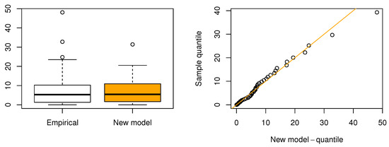
Figure 12. Box plot (left) and QQ plot (right) for the first dataset.

6.2. Dataset II

The dataset used in this analysis comprises flood frequency data provided by [47], consisting of 59 annual maximum precipitation datapoints for Karachi city, Pakistan, for the years 1950–2009 (1987 excluded). We computed the MLEs for each model, and the numerical results are presented in Table 10 and Table 11, while the information matrix of the proposed model is given below. The results indicate that the proposed distribution offers a superior fit compared to other models, as evidenced by Figure 13, where the proposed model ranks first, outperforming others in five of the seven statistical measures evaluated. Table 11 shows that the performance of the proposed model is clearly superior across all parametric evaluation metrics. It yields the highest log-likelihood value ($L=-317.43$) and achieves the lowest values for AIC (642.87), BIC (651.18), and CAIC (643.61), reflecting an optimal balance between model fit and complexity. Additionally, it records the smallest KS statistic (0.0637) with the highest associated p-value (0.9583), indicating an excellent agreement with the empirical distribution. It is followed by the MW model with L (−338.23) and KS statistic (0.0760 with p-value = 0.8611). The MWE distribution has KS statistic (0.0654) and p-value (0.9489), but its higher AIC (686.75) and BIC (692.97) indicate that it is less efficient than the proposed model in terms of model complexity. On the other hand, the AddW and GIW distributions show the weakest performance overall, with the lowest log-likelihood ($L_{GIW}=-351.69and{L}_{AddW}=-346.69$) and the poorest fit statistics ($K{S}_{GIW}=0.1466, p-value=0.1429;K{S}_{AddW}=0.1849, p-value=0.0306$), respectively, indicating their inadequacy for modeling the data. Additionally, Figure 14 displays a precise alignment with the empirical data through the fitted PDF and survival functions. Figure 15 further supports this by showing a box plot and quantile–quantile (QQ) plot, which confirm the proposed model’s compatibility with the observed data.

$$J^{-1}=\left[\begin{array}{cccc}0.02338214& -0.15017017& 0.00739371& -0.10881643\\ -0.15017017& 0.98781284& -0.04995159& 0.71398501\\ 0.00739371& -0.04995159& 0.00261462& -0.03672466\\ -0.10881643& 0.71398501& -0.03672466& 0.61016552\end{array}\right].$$

Table 10. MLEs for second dataset.

Distribution	$\mathit{\alpha }$	$\mathit{\beta }$	$\mathit{\lambda }$	$\mathit{\gamma }$	a	b
New model	0.0531 (0.1529)	0.3878 (0.9939)	-	-	0.0230 (0.0511)	0.2665 (0.7811)
	(0.00, 0.3528)	(0.00, 2.3359)	-	-	(0.00, 0.1232)	(0, 1.7975)
MW	0.0033 (0.0032)	0.0009 (0.0016)	1.1506 (0.2374)	-	-	-
	(0.00, 0.0096)	(0.00, 0.0039)	(0.6853, 1.6159)	-	-	-
EW	0.0050 (0.0119)	1.1239 (0.3943)	1.2057 (0.7357)	-	-	-
	(0.00, 0.0285)	(0.3511, 1.8967)	(0.00, 2.6477)	-	-	-
AddW	0.0001 (0.0004)	1.8459 (0.7978)	0.0064 (0.0175)	0.0575 (0.1673)	-	-
	(0.00, 0.0009)	(0.2822, 3.4097)	(0.00, 0.0407)	(0.00, 0.3858)	-	-
FW	0.0042 (0.0005)	40.6199 (4.1966)	-	-	-	-
	(0.0033, 0.0051)	(32.5947, 49.0452)	-	-	-	-
W	0.0022 (0.0015)	1.2622 (0.1315)	-	-	-	-
	(0.00, 0.0052)	(1.0044, 1.5201)	-	-	-	-
MWE	50.5310 (4.607)	0.6009 (0.0443)	0.0038 (0.0007)	-	-	-
	(46.2761, 64.3367)	(0.5139, 0.6878)	(0.0024, 0.0052)	-	-	-
GIW	5.2857 (5.070)	0.9079 (0.0832)	-	7.3235 (6.5604)	-	-
	(0.00, 15.2243)	(0.7448, 1.07124)	-	(0.00, 10.1820)	-	-
GGIW	258.86 (5.7488)	0.2069 (0.0227)	12.3762 (12.8541)	8.8677 (1.7091)	-	-
	(247.5886, 270.1215)	(0.1625, 0.2514)	(0.00, 37.5703)	(5.5180, 12.2175)	-	-
ESW	1.3412 (1.1532)	0.9944 (0.5035)	0.0057 (0.0174)	-	-	-
	(0.00, 3.6014)	(0.0074, 1.9814)	(0.00, 0.0399)	-	-	-
ECSW	0.1517 (0.0188)	0.0133 (0.0124)	1.1498 (0.0065)	-	-	-
	(0.0959, 0.1617)	(0.0307, 0.1541)	(0.8651, 1.0201)	-	-	-

Table 11. L, AIC, BIC, CAIC, A, W, KS (p-value), and rank as superscript for second dataset.

Distribution	L	$\mathit{A}\mathit{I}\mathit{C}$	$\mathit{B}\mathit{I}\mathit{C}$	$\mathit{C}\mathit{A}\mathit{I}\mathit{C}$	A	W	$\mathit{K}\mathit{S}\left(\mathit{p}\mathit{v}\right)$
New Model	−317.43 1	642.87 1	651.18 1	643.61 1	0.3308 6	0.0557 6	0.0637 1 (0.9583)
MW	−338.23 2	682.46 3	688.69 3	682.89 3	0.2482 1	0.0428 1	0.07603 (0.8611)
EW	−338.51 4	683.01 4	689.24 4	683.45 4	0.2949 3	0.0519 3	0.0982 6 (0.5854)
AddW	−346.69 10	701.39 10	709.71 10	702.14 10	0.4271 7	0.0656 7	0.1849 10 (0.0306)
FW	−342.10 9	688.19 9	692.35 7	688.41 9	0.8312 10	0.1319 10	0.1685 9 (0.0621)
W	−338.39 3	680.77 2	684.93 2	680.99 2	0.2730 2	0.0481 2	0.0807 4 (0.6933)
MWE	−340.37 7	686.75 8	692.97 8	687.18 6	0.4578 8	0.0704 8	0.0654 2 (0.9489)
GIW	−351.69 11	709.39 11	715.62 11	709.83 11	2.1687 11	0.3559 11	0.1466 8 (0.1429)
GGIW	−339.61 6	687.23 7	695.54 9	687.97 8	0.4828 9	0.0819 9	0.9925 11 (7.7$\times {10}^{-16}$)
ESW	−338.66 5	683.31 5	689.55 5	683.75 5	0.3127 4	0.0549 5	0.1002 7 (0.5598)
ECSW	−340.55 8	687.10 6	693.34 6	687.54 7	0.3283 5	0.0576 4	0.0980 5 (0.5876)

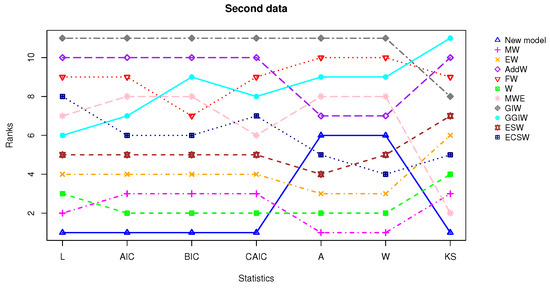
Figure 13. Line plot for ranking assessment based on the statistics for the second dataset.

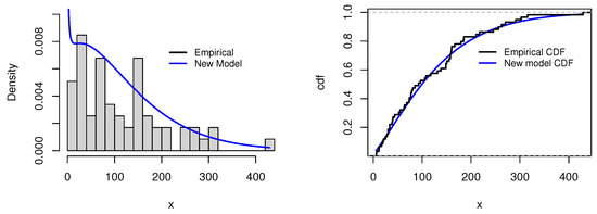
Figure 14. Visual fit assessment for the second dataset: histogram with the superimposed PDF (left) and empirically fitted CDF comparison (right).

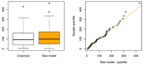
Figure 15. Box plot (left) and QQ plot (right) for the second dataset.

6.3. Dataset III

This dataset was described in [48]; it includes the daily new deaths due to COVID-19 in California, USA, collected from the month of $3/12$ to $9/30$ in the year 2020. Table 12 outlines the MLEs for each model, and the information matrix is given below, while Table 13 illustrates that the proposed distribution outperforms other models in terms of fit. The proposed distribution consistently registers more of the smallest values across evaluative criteria and goodness-of-fit measures, leading it to be ranked as the top model in Figure 16. The proposed model attains the highest log-likelihood value ($L=-1040.51$) and the lowest values for AIC (2087.04), BIC (2096.95), and CAIC (2087.18), indicating a superior trade-off between fit and complexity. Additionally, it achieves the smallest Kolmogorov–Smirnov statistic (0.0602) and a reasonable p-value (0.4597), suggesting a good agreement with the empirical distribution. Followed by AddW and EW, the EW distribution, ranking second in AIC/BIC, has a moderately larger KS statistic (0.0817) and lower p-value (0.1365), indicating a slightly weaker fit. Models such as W, ESW, and ECSW offer moderate performance but fall behind in both parsimony and goodness-of-fit measures. The ECSW model records a higher KS statistic (0.1378) with a very low p-value (0.0001), reflecting poor fit despite reasonable AIC values. In contrast, the GGIW and FW models perform the worst. The GGIW model shows the largest AIC (2337.76), BIC (2347.67), and KS statistic (0.2447), with a highly significant p-value, indicating severe misfit. Similarly, the FW model records the second-worst fit statistics (KS = 0.3541, A = 10.6004), making both models unsuitable for this dataset. This demonstrates the proposed model’s exceptional ability to adequately reflect the data, making it the most suitable model for this case of study according to these metrics. Moreover, to corroborate our conclusions, Figure 17 shows the proposed distribution’s excellent fit through the displayed fitted PDF and survival function. Additionally, Figure 18 features a box plot and a QQ plot, confirming the proposed model’s alignment with the observed data.

$$J^{-1}=\left[\begin{array}{cccc}0.00005024& -0.00309473& 0.00018684& 0.00038797\\ -0.00309473& 0.20766241& -0.01350810& -0.03257750\\ 0.00018684& -0.01350810& 0.00093729& 0.00227722\\ 0.00038797& -0.03257750& 0.00227722& 0.02763097\end{array}\right].$$

Table 12. MLEs for third dataset.

Distribution	$\mathit{\alpha }$	$\mathit{\beta }$	$\mathit{\lambda }$	$\mathit{\gamma }$	a	b
New model	0.0069 (0.0071)	0.8939 (0.4557)	-	-	0.0317 (0.0306)	0.3069 (0.1662)
	(0.00, 0.0209)	(0.0007, 1.7870)	-	-	(0.0010, 0.0917)	(0.00, 0.6328)
EW	0.0002 (0.0007)	1.8824 (0.7809)	0.7049 (0.4052)	-	-	-
	(0.0010, 0.0015)	(0.3518, 3.4131)	(0.00, 1.4991)	-	-	-
AddW	0.0162 (0.0103)	0.2495 (0.1664)	0.0004 (0.0001)	1.7323 (0.2199)	-	-
	(0.00, 0.0363)	(0.00, 0.5756)	(0.00, 0.00126)	(1.3001, 2.1634)	-	-
FW	0.0075 (0.0004)	15.2500 (2.0980)	-	-	-	-
	(0.0067, 0.0083)	(11.1408, 19.3660)	-	-	-	-
W	0.0009 (0.0004)	1.5617 (0.0937)	-	-	-	-
	(0.00010, 0.0018)	(1.3780, 1.7453)	-	-	-	-
GIW	1.3837 (1.1204)	0.7117 (0.0311)	-	9.5355 (5.3508)	-	-
	(0.00, 3.5798)	(0.6506, 0.7728)	(0.00, 20.0239)	-	-	-
GGIW	936.52 (5.3450)	0.1918 (0.0100)	13.5043 (0.1426)	9.6692 (0.2226)	-	-
	(926.045, 946.998)	(0.1722, 0.2114)	(13.2248, 13.7830)	(9.2328, 10.1055)	-	-
ESW	0.9210 (0.4955)	1.4512 (0.5615)	0.0007 (0.0021)	-	-	-
	(0.00, 1.8922)	(0.3906, 2.5917)	(0.00, 0.0047)	-	-	-
ECSW	0.08524 (0.0060)	0.0571 (0.0001)	1.1020 (0.00001)	-	-	-
	(0.0735, 0.0970)	(0.0537, 0.0538)	(1.1022, 1.2023)	-	-	-

Table 13. L, AIC, BIC, CAIC, A, W, KS (p-value), and rank as superscript for third dataset.

Distribution	L	$\mathit{A}\mathit{I}\mathit{C}$	$\mathit{B}\mathit{I}\mathit{C}$	CAIC	A	W	$\mathit{K}\mathit{S}\left(\mathit{p}\mathit{v}\right)$
New Model	−1040.51 1	2087.04 1	2096.95 1	2087.18 1	1.0651 3	0.1765 3	0.0602 1 (0.4597)
EW	−1050.21 2	2106.42 2	2116.33 2	2106.54 2	0.9581 2	0.1550 2	0.0817 3 (0.1365)
AddW	−1050.54 3	2109.07 3	2122.29 5	2109.28 3	0.7447 1	0.1132 1	0.0627 2 (0.4080)
FW	−1145.42 8	2294.85 8	2301.45 8	2294.91 8	10.6004 8	1.7262 8	0.3541 9 (1.0$\times {10}^{-24}$)
W	−1053.59 5	2111.17 5	2117.78 3	2111.23 5	1.3337 5	0.2181 5	0.0825 4 (0.1294)
GIW	−1070.39 7	2148.78 7	2161.59 7	2148.99 7	3.7133 7	0.6079 7	0.9999 8 (1.0$\times {10}^{-24}$)
GGIW	−1165.88 9	2337.76 9	2347.67 9	2337.89 9	17.0667 9	2.9720 9	0.2447 7 (6.9$\times {10}^{-11}$)
ESW	−1052.00 4	2110.01 4	2119.92 4	2110.13 4	1.1570 4	0.1870 4	0.0880 6 (0.0892)
ECSW	−1069.47 6	2144.86 6	2154.86 6	2145.07 6	2.2423 6	0.3765 6	0.8143 5 (3.4$\times {10}^{-16}$)

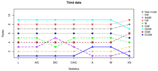
Figure 16. Line plot for ranking assessment based on the statistics for the third dataset.

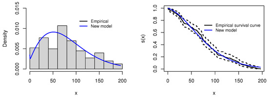
Figure 17. Visual fit assessment for the third dataset: histogram with the superimposed PDF (left) and empirically fitted CDF comparison (right).

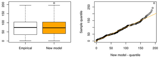
Figure 18. Box plot (left) and QQ plot (right) for the third dataset.

7. Conclusions and Future Studies

This study proposed a novel four-parameter probability distribution called integrated linear–Weibull and explored its fundamental mathematical characteristics, including expressions for the moments, mean residual life and its asymptotic, order statistics, extropy, and cumulative residual entropy. The identifiability of the model was validated numerically via the Kullback–Leibler divergence for selected parameter settings, confirming that the model’s parameters can be uniquely identified under the assumed conditions. The stress–strength reliability parameter was also derived under the assumption of independence between two random variables with differing scale parameters. Parameter estimation was performed using the MLE method, and a comprehensive simulation study was conducted to evaluate the estimators. The results show that the bias and MSE decrease as the sample size increases, demonstrating the consistency and efficiency of the MLEs. The practical utility of the proposed model was further validated using two real-life datasets. In both applications, the model outperformed several existing alternatives, highlighting its flexibility and suitability in applied statistical modeling.

This work not only demonstrates the flexibility and strong performance of the proposed distribution but also provides a foundation for several avenues of future research. Potential extensions include developing alternative models with various methods, such as exponentiation and trigonometric-G or multivariate generalizations. In addition, other methods include Bayesian estimation under censoring and exploring additional reliability measures, including mean residual life analysis and stress–strength modeling. Further applied investigations, particularly in hydrology, environmental extremes, and biomedical survival studies, could be explored using the proposed distribution.

Even though the ILW model is flexible and performs well empirically, every extended distribution has some structural limitations. The ILW model inherits a non-explicit quantile function; thus, it requires numerical inversion to sample random data. In addition, ILW has some computational intensity for higher-order properties, as shown for identifiability in Section 2.6. Furthermore, the standard errors depend on numerical differentiation (hessian function in the package ‘numDeriv’ in R-software is sufficient [38]) or computation of some complex second derivatives because it is intractable to obtain a closed-form expected Fisher information matrix.

References

- Meeker, W.Q.; Escobar, L.A.; Pascual, F.G. Statistical Methods for Reliability Data; John Wiley & Sons: Hoboken, NJ, USA, 2022. [Google Scholar]
- Murthy, D.P.; Xie, M.; Jiang, R. Weibull Models; John Wiley & Sons: Hoboken, NJ, USA, 2004. [Google Scholar]
- Lai, C.D.; Murthy, D.N.P.; Xie, M. Weibull distributions. WIREs Comput. Stat. 2011, 3, 282–287. [Google Scholar] [CrossRef]
- Lai, C.D.; Zhang, L.; Xie, M. Mean residual life and other properties of Weibull related bathtub shape failure rate distributions. Int. J. Reliab. Qual. Saf. Eng. 2004, 11, 113–132. [Google Scholar] [CrossRef]
- Pal, M.; Ali, M.M.; Woo, J. Exponentiated Weibull distribution. Statistica 2006, 66, 139–147. [Google Scholar]
- Abd EL-Baset, A.A.; Ghazal, M. Exponentiated additive Weibull distribution. Reliab. Eng. Syst. Saf. 2020, 193, 106663. [Google Scholar] [CrossRef]
- Alsulami, D.; Alghamdi, A.S. A New Extended Weibull Distribution: Estimation Methods and Applications in Engineering, Physics, and Medicine. Mathematics 2025, 13, 3262. [Google Scholar] [CrossRef]
- Alshanbari, H.M.; Ahmad, Z.; El-Bagoury, A.A.A.H.; Odhah, O.H.; Rao, G.S. A New Modification of the Weibull Distribution: Model, Theory, and Analyzing Engineering Data Sets. Symmetry 2024, 16, 611. [Google Scholar] [CrossRef]
- Mastor, A.B.S.; Ngesa, O.; Mung’atu, J.; Alfaer, N.M.; Afify, A.Z. The Extended Exponential Weibull Distribution: Properties, Inference, and Applications to Real-Life Data. Complexity 2022, 2022, 4068842. [Google Scholar] [CrossRef]
- El-Morshedy, M.; El-Dawoody, M.; El-Faheem, A.A. Symmetric and Asymmetric Expansion of the Weibull Distribution: Features and Applications to Complete, Upper Record, and Type-II Right-Censored Data. Symmetry 2025, 17, 131. [Google Scholar] [CrossRef]
- Xu, M.; Mao, H. q-Weibull Distributions: Perspectives and Applications in Reliability Engineering. IEEE Trans. Reliab. 2025, 74, 3112–3125. [Google Scholar] [CrossRef]
- Wang, H.; Abba, B.; Pan, J. Classical and Bayesian estimations of improved Weibull–Weibull distribution for complete and censored failure times data. Appl. Stoch. Model. Bus. Ind. 2022, 38, 997–1018. [Google Scholar] [CrossRef]
- Abba, B.; Wu, J.; Muhammad, M. A robust multi-risk model and its reliability relevance: A Bayes study with Hamiltonian Monte Carlo methodology. Reliab. Eng. Syst. Saf. 2024, 250, 110310. [Google Scholar] [CrossRef]
- Noori, N.A.; Abdullah, K.N.; Khaleel, M.A. Development and Applications of a New Hybrid Weibull-Inverse Weibull Distribution. Mod. J. Stat. 2025, 1, 80–103. [Google Scholar] [CrossRef]
- Muhammad, M.; Xiao, J.; Abba, B.; Muhammad, I.; Ghodhbani, R. A New Hybrid Class of Distributions: Model Characteristics and Stress–Strength Reliability Studies. Axioms 2025, 14, 219. [Google Scholar] [CrossRef]
- Shah, Z.; Khan, D.M.; Khan, Z.; Shafiq, M.; Choi, J.G. A New Modified Exponent Power Alpha Family of Distributions with Applications in Reliability Engineering. Processes 2022, 10, 2250. [Google Scholar] [CrossRef]
- Alshanbari, H.M.; Al-Mofleh, H.; Seong, J.T.; Khosa, S.K. A New Tangent-Generated Probabilistic Approach with Symmetrical and Asymmetrical Natures: Monte Carlo Simulation with Reliability Applications. Symmetry 2023, 15, 2066. [Google Scholar] [CrossRef]
- Meredith, M.; Kruschke, J. HDInterval: Highest (posterior) density intervals. In CRAN: Contributed Packages; CRAN: Vienna, Austria, 2016. [Google Scholar]
- Gradshteyn, I.S.; Ryzhik, I.M. Table of Integrals, Series, and Products; Academic Press: Cambridge, MA, USA, 2014. [Google Scholar]
- Barlow, R. Statistical theory of reliability and life testing. Holt. 1975. Available online: https://cir.nii.ac.jp/crid/1570854174228233472 (accessed on 8 December 2025).
- Guess, F.; Proschan, F. 12 mean residual life: Theory and applications. Handb. Stat. 1988, 7, 215–224. [Google Scholar]
- Xie, M.; Goh, T.N.; Tang, Y. On changing points of mean residual life and failure rate function for some generalized Weibull distributions. Reliab. Eng. Syst. Saf. 2004, 84, 293–299. [Google Scholar] [CrossRef]
- Olcay, A.H. Mean residual life function for certain types of non-monotonic ageing. Commun. Stat. Stoch. Model. 1995, 11, 219–225. [Google Scholar] [CrossRef]
- Calabria, R.; Pulcini, G. On the maximum likelihood and least-squares estimation in the inverse Weibull distribution. Stat. Appl. 1990, 2, 53–66. [Google Scholar]
- Shakhatreh, M.K.; Lemonte, A.J.; Moreno-Arenas, G. The log-normal modified Weibull distribution and its reliability implications. Reliab. Eng. Syst. Saf. 2019, 188, 6–22. [Google Scholar] [CrossRef]
- Ito, C.; Maeda, T.; Higashi, R.; Osada, T.; Kohata, T.; Ozaki, S. Application of extreme value statistics to internal pore distribution in ceramics and prediction of size dependency of strength scatter. J. Eur. Ceram. Soc. 2024, 44, 3381–3392. [Google Scholar] [CrossRef]
- Arnold, B.C.; Balakrishnan, N.; Nagaraja, H.N. A First Course in Order Statistics; SIAM: Philadelphia, PA, USA, 1992; Volume 54. [Google Scholar]
- Ran, Z.Y.; Hu, B.G. Determining parameter identifiability from the optimization theory framework: A Kullback–Leibler divergence approach. Neurocomputing 2014, 142, 307–317. [Google Scholar] [CrossRef]
- Lad, F.; Sanfilippo, G.; Agro, G. Extropy: Complementary dual of entropy. Stat. Sci. 2015, 30, 40–58. [Google Scholar] [CrossRef]
- Xue, Y.; Deng, Y. Tsallis extropy. Commun. Stat.-Theory Methods 2023, 52, 751–762. [Google Scholar] [CrossRef]
- Tahmasebi, S.; Toomaj, A. On negative cumulative extropy with applications. Commun. Stat.-Theory Methods 2022, 51, 5025–5047. [Google Scholar] [CrossRef]
- Kotz, S.; Lumelskii, Y.; Pensky, M. The Stress–Strength Model and Its Generalizations: Theory and Applications; World Scientific: Singapore, 2003. [Google Scholar]
- Saber, M.M.; Mohie El-Din, M.M.; Yousof, H.M. Reliability Estimation for the Remained Stress-Strength Model Under the Generalized Exponential Lifetime Distribution. J. Probab. Stat. 2021, 2021, 7363449. [Google Scholar] [CrossRef]
- Garg, R.; Kumari, M.; Sahoo, R.K.; Kumari, A. Stress-strength reliability estimation of multicomponent system with non-identical strength components from inverse Pareto distribution. Life Cycle Reliab. Saf. Eng. 2024, 13, 351–363. [Google Scholar] [CrossRef]
- Muhammad, I.; Wang, X.; Li, C.; Yan, M.; Chang, M. Estimation of the reliability of a stress–strength system from Poisson half logistic distribution. Entropy 2020, 22, 1307. [Google Scholar] [CrossRef] [PubMed]
- Ahmadi, M.V. Estimating stress-strength reliability based on two-parameter exponential records in the presence of inter-record times. Qual. Technol. Quant. Manag. 2025, 22, 993–1024. [Google Scholar] [CrossRef]
- Henningsen, A.; Toomet, O. maxLik: A package for maximum likelihood estimation in R. Comput. Stat. 2011, 26, 443–458. [Google Scholar] [CrossRef]
- Gilbert, P.; Varadhan, R.; Gilbert, M.P. Package ‘numDeriv’. Differ. Equ. 2009, 3, 203–267. [Google Scholar]
- Lai, C.; Xie, M.; Murthy, D. A modified Weibull distribution. IEEE Trans. Reliab. 2003, 52, 33–37. [Google Scholar] [CrossRef]
- Bebbington, M.; Lai, C.D.; Zitikis, R. A flexible Weibull extension. Reliab. Eng. Syst. Saf. 2007, 92, 719–726. [Google Scholar] [CrossRef]
- Xie, M.; Lai, C.D. Reliability analysis using an additive Weibull model with bathtub-shaped failure rate function. Reliab. Eng. Syst. Saf. 1996, 52, 87–93. [Google Scholar] [CrossRef]
- Xie, M.; Tang, Y.; Goh, T.N. A modified Weibull extension with bathtub-shaped failure rate function. Reliab. Eng. Syst. Saf. 2002, 76, 279–285. [Google Scholar] [CrossRef]
- Muhammad, M.; Alshanbari, H.M.; Alanzi, A.R.; Liu, L.; Sami, W.; Chesneau, C.; Jamal, F. A new generator of probability models: The exponentiated sine-G family for lifetime studies. Entropy 2021, 23, 1394. [Google Scholar] [CrossRef]
- Muhammad, M.; Bantan, R.A.; Liu, L.; Chesneau, C.; Tahir, M.H.; Jamal, F.; Elgarhy, M. A new extended cosine—G distributions for lifetime studies. Mathematics 2021, 9, 2758. [Google Scholar] [CrossRef]
- De Gusmao, F.R.; Ortega, E.M.; Cordeiro, G.M. The generalized inverse Weibull distribution. Stat. Pap. 2011, 52, 591–619. [Google Scholar] [CrossRef]
- Jain, K.; Singla, N.; Sharma, S.K. The generalized inverse generalized Weibull distribution and its properties. J. Probab. 2014, 2014, 736101. [Google Scholar] [CrossRef]
- Bhatti, F.A.; Hamedani, G.; Ali, A.; Ahmad, M. On the generalized log Burr III distribution: Development, properties, characterizations and applications. Pak. J. Stat. 2019, 35, 25–51. [Google Scholar]
- Muhammad, M.; Liu, L.; Abba, B.; Muhammad, I.; Bouchane, M.; Zhang, H.; Musa, S. A new extension of the Topp–Leone-family of models with applications to real data. Ann. Data Sci. 2023, 10, 225–250. [Google Scholar] [CrossRef] [PubMed]
Disclaimer/Publisher’s Note: The statements, opinions and data contained in all publications are solely those of the individual author(s) and contributor(s) and not of MDPI and/or the editor(s). MDPI and/or the editor(s) disclaim responsibility for any injury to people or property resulting from any ideas, methods, instructions or products referred to in the content. |
© 2025 by the authors. Licensee MDPI, Basel, Switzerland. This article is an open access article distributed under the terms and conditions of the Creative Commons Attribution (CC BY) license (https://creativecommons.org/licenses/by/4.0/).