Stem Structures and Novel Localized Wave Molecules of the (2+1)-Dimensional pKP-BKP Equation

Abstract

In this paper, asymptotic analysis for the (2+1)-dimensional potential Kadomtsev Petviashvili B-type Kadomtsev Petviashvili (pKP-BKP) equation is conducted to establish this limiting. The study examines the stem structures resulting from resonance collisions of the two-soliton solution in the (2+1)-dimensional pKP-BKP equation. The trajectories, amplitudes and velocities of the soliton arms and the lengths of the stem structures are calculated through asymptotic analysis. By combining the characteristic line analysis and the velocity resonance mechanism, novel bound states consisting of transformed wave–soliton molecules and transformed wave molecules are systematically constructed. These results provide explicit insight into the formation and evolution of localized nonlinear waves in the pKP-BKP system, and they offer a concrete theoretical foundation for wave resonance and bound states in higher-dimensional dispersive media.

1. Introduction

Nonlinear differential equations are fundamental to integrable systems, modeling diverse physical phenomena such as fluid dynamics, optical fibers and plasma physics [1,2,3,4]. Symmetry plays a pivotal role in revealing the intrinsic structure and determining the integrability of nonlinear differential equations [5]. A nonlinear system is often regarded as integrable when it possesses infinitely many Lie symmetries or master symmetries, which generate hierarchies of commuting flows and conservation laws. Techniques like the inverse scattering transform [6], Hirota’s bilinear method [7], symmetry reductions [8] and Darboux transformation [9] have been developed to analyze and solve these equations. Nonlinear equations have been frequently studied due to their significance in integrable systems, including the nonlinear Schrödinger (NLS) equation [10], the Korteweg-de Vries equation [11], the Kadomtsev–Petviashvili equation [12], the sine-Gordon equation [13] and the Boussinesq equation [14]. The solutions of nonlinear differential equations often exhibit intriguing phenomena. Solitons are stable and localized wave packets maintain their shape during propagation [15]. Breathers are periodic solutions that exhibit oscillatory behavior without spreading [16]. Lump waves are localized waves with a more intricate structure and can describe energy transfer phenomena in nonlinear media [17].

The elastic interaction between two intersecting solitons can lead to the formation of an X-shaped structure, commonly known as an X-shaped soliton. A distinguishing feature of such solitons is the induction of finite phase shifts during the collision process. When the phase shift tends toward infinity, a resonance phenomenon occurs, resulting in the emergence of a novel isolated wave that connects two V-shaped regions [18,19]. In particular, the occurrence of infinite phase shifts gives rise to Y-shaped solitons [20], which have been observed in various natural environments [21].

Previous studies have reported that certain nonlinear waves can undergo transformation into other wave types in nonlinear equations containing higher-order nonlinear and dispersive terms. Chowdury et al. proposed a physical mechanism in which a breather can be converted into a soliton within the integrable hierarchy of the NLS equation [22]. Wang et al. found that breathers, rogue waves and semirational solutions of the higher-order generalized NLS equation could transition into nonpulsating soliton solutions [23]. Chowdury et al. demonstrated that a breather solution of the NLS hierarchy includes fifth-order dispersion with matching higher-order nonlinear terms and could be converted into a nonpulsating soliton solution on a background [24]. Huang et al. revealed a breather-to-soliton transition in a sixth-order NLS equation within an optical fiber [25]. For high-dimensional space, Liu et al. derived that a breather can transition into a soliton in the (2+1)-dimensional Ito equation [26]. The breather can also be converted into a soliton in the (2+1)-dimensional Korteweg–de Vries–Sawada–Kotera–Ramani equation [27]. Ma et al. investigated breather-to-soliton transitions in a nonlinear (3+1)-dimensional shallow water wave equation [28]. The transformed waves of the (3+1)-dimensional Boiti–Leon–Manna–Pempinelli equation are proposed [29].

Building upon the rich dynamics of nonlinear wave phenomena, soliton molecules represent a fascinating class of bound states in integrable systems. In contrast to isolated solitons, soliton molecules are composed of two or more solitons that remain stably bound through specific nonlinear interactions. The formation of such bound states typically necessitates that the constituent solitons possess identical or nearly identical group velocities, ensuring their synchronization during propagation. These structures have been extensively investigated across various nonlinear systems. Notably, soliton molecules have been experimentally observed in optical fibers, exhibiting robust stability even in the presence of perturbations. Krupa et al. presented the evidence of the internal motion of a dissipative optical soliton molecule generated in a passively mode locked erbium-doped fiber laser [30]. Stratmann et al. demonstrated the stable formation of temporal soliton bound states within optical fibers [31]. Herink et al. explored the dynamics of femtosecond soliton molecules in mode-locked lasers [32]. For theoretical work, the velocity resonance mechanism provides an effective method for constructing and analyzing soliton molecules [33,34,35].

In this paper, we consider a combined (2+1)-dimensional potential Kadomtsev–Petviashvili-B-type Kadomtsev–Petviashvili equation [36], which is used to describe weakly dispersive waves propagating in fluid mechanics. It reads as:

$$\begin{array}{cc}\hfill & {\alpha }_1{(15u_x^3+15u_x{u}_{xxx}+u_{xxxxx})}_x+{\alpha }_2(6u_x{u}_{xx}+u_{xxxx})+{\alpha }_3\left(u_{xxxy}+3{\left(u_x{u}_y\right)}_x\right)\\ & +{\alpha }_4{u}_{xx}+{\alpha }_5{u}_{xt}+{\alpha }_6{u}_{yy}=0,\end{array}$$

(1)

where the parameters ${\alpha }_j(j=1\dots 6)$ are arbitrary real constants. The (2+1)-dimensional pKP-BKP equation has drawn increasing attention due to its rich nonlinear structures and physical relevance [37,38,39,40,41]. Various types of exact solutions have been obtained using the Hirota’s bilinear method, including lump, breather, and lump–soliton interaction solutions [37]. Additionally, by means of Bäcklund transformations and symbolic computation, researchers have derived complexions, kink solitons, and breather solutions, with their dynamics visualized through three-dimensional and contour plots [38]. Transformation mechanisms and nonlinear interactions such as wave conversion, oscillation, and molecule formation have also been explored using geometric and resonance-based approaches [39]. Feng et al. derived the multi-breather solution based on the N-soliton solution [40]. Wazwaz et al. obtained lump, periodic and double-kink soliton solutions of the Equation (1) [41]. In contrast to the classical KP-type equations, the pKP-BKP equation studied in this paper includes higher-order dispersive and nonlinear terms, enabling the emergence of richer nonlinear dynamics. While previous studies have reported transformed waves and soliton molecules in KP-type systems, these works mostly focus on lower-order models or rely on numerical simulations. In this paper, we systematically construct some novel localized molecules based on the multi-soliton of the pKP-BKP system. Specifically, the generation of M-shaped solitons, oscillation solitons, and quasi-periodic waves through parameter modulation, as well as the analytical derivation of X-shaped and Y-shaped resonance structures with quantitative stem-length formulas, distinguishes our work from existing literature. Furthermore, we propose a new family of composite bound states by applying the velocity resonance mechanism. These structures have not been reported in the pKP-BKP context or in traditional KP-type models. These developments contribute new theoretical perspectives on wave interactions in higher-dimensional integrable systems.

In addition to their mathematical interest, the nonlinear structures revealed in this work have meaningful implications for engineering applications. The pKP-BKP model and its variants arise naturally in physical contexts such as the shallow-water wave dynamics, the internal waves in the stratified fluids, the plasma physics, and the optical wave-guides for the nonlinear dispersive media. In these systems, the formation of X-shaped and Y-shaped resonant solitons, as well as localized wave molecules, is directly related to energy focusing and signal propagation stability. The explicit formulas obtained in this paper for the stem length, soliton trajectories, resonance conditions and molecule-type bound states provide concrete predictive tools for understanding how localized energy packets evolve and interact in higher-dimensional environments. The nonlinear resonance and multi-peak bound states play a crucial role in the coastal engineering, the optical communication platforms and fluid structure. These results may facilitate the design and analysis of engineering systems.

The paper is organized as follows. In Section 2, the X-shaped and Y-shaped solitons are obtained by using the asymptotic analysis method. In addition, the expressions for the velocity, amplitude, and trajectory of these solitons are provided. In Section 3, some mixed solutions composed of breathers, solitons and transformed waves are presented by combining the complex conjugate relations and characteristic line analysis method. In Section 4, the bound state molecules including the transformed wave–soliton and transformed wave molecule are constructed by applying the velocity resonance conditions. Finally, the conclusion is given in Section 5.

2. Stem Structures of the (2+1)-Dimensional pKP-BKP Equation

In this section, the N-soliton solution is derived using Hirota’s bilinear method. Asymptotic analysis reveals the phase shifts resulting from the collision of two solitons. It leads to two specific types of solitons.

By using the transformation

$$\begin{array}{c}\hfill v=u_x=2{(lnf)}_{xx},\end{array}$$

(2)

where v is a potential function; the bilinear form of the pKP-BKP equation is given by [36]:

$$\begin{array}{c}\hfill ({\alpha }_1{D}_x^6+{\alpha }_2{D}_x^4+{\alpha }_3{D}_x^3{D}_y+{\alpha }_4{D}_x^2+{\alpha }_5{D}_x{D}_t+{\alpha }_6{D}_y^2)f·f=0,\end{array}$$

where $D_t,D_x$ and $D_y$ are the Hirota bilinear operators. Under this condition, ${\alpha }_3^2+5{\alpha }_1{\alpha }_6=0$; the expression for the N-soliton solution of the above equation is as follows:

$$\begin{array}{c}\hfill f=f_N=\sum _{\mu =0,1}exp(\sum _{i=1}^N{\mu }_i{\eta }_i+\sum _{i<j}^N{\mu }_i{\mu }_j{A}_{ij}),\end{array}$$

(3)

with

$$\begin{array}{cc}\hfill & {\eta }_i=k_i(x+p_{i}y+{\omega }_{i}t)+{\varphi }_i,{\omega }_i=-({\displaystyle \frac{{\alpha }_1{k}_i^4+{\alpha }_3{k}_i^2{p}_i+{\alpha }_2{k}_i^2+{\alpha }_6{p}_i^2+{\alpha }_4}{{\alpha }_5}}),{\alpha }_5\ne 0,\\ & exp\left(A_{ij}\right)=-{\displaystyle \frac{{\alpha }_1{(k_i-k_j)}^6+{\alpha }_2{(k_i-k_j)}^4+{\alpha }_3{(k_i-k_j)}^3(k_i{p}_i-k_j{p}_j)+{\alpha }_4{(k_i-k_j)}^2+{\alpha }_5(k_i-k_j)(k_i{\omega }_i-k_j{\omega }_j)+{\alpha }_6{(k_i{p}_i-k_j{p}_j)}^2}{{\alpha }_1{(k_i+k_j)}^6+{\alpha }_2{(k_i+k_j)}^4+{\alpha }_3{(k_i+k_j)}^3(k_i{p}_i+k_j{p}_j)+{\alpha }_4{(k_i+k_j)}^2+{\alpha }_5(k_i+k_j)(k_i{\omega }_i+k_j{\omega }_j)+{\alpha }_6{(k_i{p}_i+k_j{p}_j)}^2}},\end{array}$$

(4)

where $k_i$ determines the amplitude of the soliton and is directly related to its propagation characteristics in the x direction, while $p_i$ regulates the soliton’s transverse (y-direction) propagation characteristics. By employing asymptotic analysis for the two-soliton solution ($N=2$ in Equation (3)), the expressions of the soliton solutions before and after the collision are derived as:

$$\begin{array}{ccc}\hfill & & S^{1-}(f_2\approx 1+exp\left({\eta }_1\right)):v^{1-}\approx {\displaystyle \frac{k_1^2}{2}}{sech}^2({\displaystyle \frac{{\eta }_1}{2}}),({\eta }_1\approx 0,{\eta }_2\to -\infty ),\hfill \\ & & S^{1+}(f_2\approx 1+a_{12}exp\left({\eta }_1\right)):v^{1+}\approx {\displaystyle \frac{k_1^2}{2}}{sech}^2({\displaystyle \frac{{\eta }_1+ln\left(a_{12}\right)}{2}}),({\eta }_1\approx 0,{\eta }_2\to +\infty ),\hfill \\ & & S^{2-}(f_2\approx 1+a_{12}exp\left({\eta }_2\right)):v^{2-}\approx {\displaystyle \frac{k_2^2}{2}}{sech}^2({\displaystyle \frac{{\eta }_2+ln\left(a_{12}\right)}{2}}),({\eta }_2\approx 0,{\eta }_1\to +\infty ),\hfill \\ & & S^{2+}(f_2\approx 1+exp\left({\eta }_2\right)):v^{2+}\approx {\displaystyle \frac{k_2^2}{2}}{sech}^2({\displaystyle \frac{{\eta }_2}{2}}),({\eta }_2\approx 0,{\eta }_1\to -\infty ),\hfill \end{array}$$

(5)

where $exp\left(A_{12}\right)\triangleq a_{12}$. The analysis shows that the phase shift of the two-soliton is $ln\left(a_{12}\right)$. As the phase shift approaches infinity, the interaction region between the two solitons becomes increasingly extended, leading to the formation of an X-shaped soliton. A localized stem structure is formed under the condition $a_{12}\approx 0$ or $a_{12}\approx \infty$. It is well known that the elastic collision of two solitons gives rise to an X-shaped soliton. Under these specific conditions, the vertex of the X-shaped soliton splits into two distinct points, and a localized stem structure emerges, connecting two V-shaped regions.

For $a_{12}\approx 0$, the special X-shaped soliton is shown in Figure 1. It is referred to a weak resonant collision. Points A and B in Figure 1 represent the vertices of the V-shaped region. It can be determined by solving the following systems of trajectory equations:

$$\begin{array}{c}\hfill \left\{\begin{array}{c}{\eta }_1=0,\hfill \\ {\eta }_2=0,\hfill \end{array}\right.\end{array}$$

(6)

and

$$\begin{array}{c}\hfill \left\{\begin{array}{c}{\eta }_1+ln\left(a_{12}\right)=0,\hfill \\ {\eta }_2+ln\left(a_{12}\right)=0.\hfill \end{array}\right.\end{array}$$

(7)

Solving these systems separately yields the coordinates of A and B as follows:

$$\begin{array}{cc}& A:({\displaystyle \frac{P}{(k_1{p}_2-k_2{p}_1){\alpha }_5}}+{\displaystyle \frac{p_1{\varphi }_2-p_2{\varphi }_1}{k_1{p}_2-k_2{p}_1}},{\displaystyle \frac{Q}{(k_1{p}_2-k_2{p}_1){\alpha }_5}}-{\displaystyle \frac{k_1{\varphi }_2-k_2{\varphi }_1}{k_1{p}_2-k_2{p}_1}}),\\ & B:({\displaystyle \frac{P}{(k_1{p}_2-k_2{p}_1){\alpha }_5}}+{\displaystyle \frac{ln\left(a_{12}\right)(p_1-p_2)+p_1{\varphi }_2-p_2{\varphi }_1}{k_1{p}_2-k_2{p}_1}},{\displaystyle \frac{Q}{(k_1{p}_2-k_2{p}_1){\alpha }_5}}-{\displaystyle \frac{ln\left(a_{12}\right)(k_1-k_2)-(k_1{\varphi }_2-k_2{\varphi }_1)}{k_1{p}_2-k_2{p}_1}}),\end{array}$$

with

$$\begin{array}{ccc}& & P=(k_1^4{p}_2-k_2^4{p}_1)t{\alpha }_1+(k_1^2{p}_2-k_2^2{p}_1)t{\alpha }_2+(k_1^2-k_2^2)p_1{p}_{2}t{\alpha }_3-(p_1-p_2)t{\alpha }_4+(p_1^2{p}_2-p_2^2{p}_1)t{\alpha }_6,\hfill \\ & & Q=(k_1{k}_2^4-k_1^4{k}_2)t{\alpha }_1-(k_1^2{k}_2-k_1{k}_2^2)t{\alpha }_2-(k_1^2{k}_2{p}_1-k_1{k}_2^2{p}_2)t{\alpha }_3+(k_1-k_2)t{\alpha }_4+(k_1{p}_2^2-k_2{p}_1^2)t{\alpha }_6.\hfill \end{array}$$

The length of the stem structure is equivalent to the distance between points A and B:

$$\begin{array}{c}\hfill \left|AB\right|=\left|{\displaystyle \frac{ln{a}_{12}}{k_1{p}_2-k_2{p}_1}}\right|\sqrt{{(k_1-k_2)}^2+{(p_1-p_2)}^2},\end{array}$$

(8)

where $k_1{p}_2\ne k_2{p}_1$.

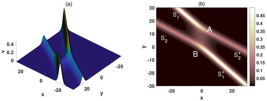
Figure 1. (a) The weak resonance collision of two-soliton with $a_{12}\approx 0$, $t=0$, ${\alpha }_1=-1$, ${\alpha }_2=1$, ${\alpha }_3=5$, ${\alpha }_4=2$, ${\alpha }_5=1$, ${\alpha }_6=5$, $k_1=1$, $k_2={\displaystyle \frac{3}{5}}$, $p_1=1$, $p_2=1.64$. (b) The density figure of (a).

The stem structure is expressed as:

$$\begin{array}{c}\hfill S^{1-2}(f_2\approx exp\left({\eta }_1\right)+exp\left({\eta }_2\right)):v^{1-2}\approx {\displaystyle \frac{{(k_1-k_2)}^2}{2}}{sech}^2({\displaystyle \frac{{\eta }_1-{\eta }_2}{2}}),({\eta }_1\approx {\eta }_2,{\eta }_{1,2}\to +\infty ).\end{array}$$

For $a_{12}\approx \infty$, the expression of the stem structure is written as

$$\begin{array}{c}\hfill S^{1+2}(f_2\approx 1+a_{12}exp({\eta }_1+{\eta }_2)):v^{1+2}\approx {\displaystyle \frac{{(k_1+k_2)}^2}{2}}{sech}^2({\displaystyle \frac{{\eta }_1+{\eta }_2+ln\left(a_{12}\right)}{2}}),({\eta }_1\approx -{\eta }_2,{\eta }_1\to +\infty ).\end{array}$$

The coordinates of vertices C and D can be determined by solving the following systems:

$$\begin{array}{c}\hfill \left\{\begin{array}{c}{\eta }_1=0,\hfill \\ {\eta }_2+ln\left(a_{12}\right)=0,\hfill \end{array}\right.\end{array}$$

(9)

and

$$\begin{array}{c}\hfill \left\{\begin{array}{c}{\eta }_1+ln\left(a_{12}\right)=0,\hfill \\ {\eta }_2=0.\hfill \end{array}\right.\end{array}$$

(10)

The corresponding points read follows as:

$$\begin{array}{cc}& C:({\displaystyle \frac{P}{(k_1{p}_2-k_2{p}_1){\alpha }_5}}+{\displaystyle \frac{ln\left(a_{12}\right)p_1+p_1{\varphi }_2-p_2{\varphi }_1}{(k_1{p}_2-k_2{p}_1)}},{\displaystyle \frac{Q}{(k_1{p}_2-k_2{p}_1){\alpha }_5}}-{\displaystyle \frac{ln\left(a_{12}\right)k_1+k_1{\varphi }_2-k_2{\varphi }_1}{(k_1{p}_2-k_2{p}_1)}}),\\ & D:({\displaystyle \frac{P}{(k_1{p}_2-k_2{p}_1){\alpha }_5}}-{\displaystyle \frac{ln\left(a_{12}\right)p_2-p_1{\varphi }_2+p_2{\varphi }_1}{k_1{p}_2-k_2{p}_1}},{\displaystyle \frac{Q}{(k_1{p}_2-k_2{p}_1){\alpha }_5}}+{\displaystyle \frac{ln\left(a_{12}\right)k_2-k_1{\varphi }_2+k_2{\varphi }_1}{k_1{p}_2-k_2{p}_1}}).\end{array}$$

(11)

The distance between points C and D is:

$$\begin{array}{c}\hfill \left|CD\right|=\left|{\displaystyle \frac{ln{a}_{12}}{k_1{p}_2-k_2{p}_1}}\right|\sqrt{{(k_1+k_2)}^2+{(p_1+p_2)}^2}.\end{array}$$

(12)

Figure 2 presents the strong resonance soliton for $a_{12}\approx \infty$. From Equations (8) and (12), it can be seen that the length of the stem is constant. It is well established that a soliton can be regarded as a traveling wave. Accordingly, the associated stem structure maintains its shape during propagation. As illustrated in Figure 1 and Figure 2, the interaction between the two solitons is confined to a localized region which is named as the stem structure. Notably, the length of the stem structure remains temporally invariant. The corresponding trajectories, amplitudes, and velocities of each soliton arm are summarized in Table 1.

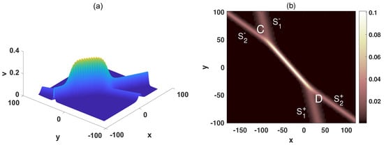
Figure 2. (a) The strong resonance collision of two-soliton with $a_{12}\approx \infty$, $t=0$, ${\alpha }_1=-1$, ${\alpha }_2=1$, ${\alpha }_3=5$, ${\alpha }_4=2$, ${\alpha }_5=1$, ${\alpha }_6=5$, $k_1={\displaystyle \frac{1}{3}}$, $k_2={\displaystyle \frac{1}{2}}$, $p_1={\displaystyle \frac{1}{3}}$, $p_2=1.21$. (b) The density figure of (a).

Table 1. Physical quantities of the X-shaped soliton arms.

Soliton	Trajectory	Velocity	Amplitude	Component
$S_1^{-}$	${\eta }_1=0$	$\left({\omega }_1,{\displaystyle \frac{{\omega }_1}{p_1}}\right)$	${\displaystyle \frac{k_1^2}{2}}$	$v_1^{-}$
$S_1^{+}$	${\eta }_1+ln\left(a_{12}\right)=0$	$\left({\omega }_1,{\displaystyle \frac{{\omega }_1}{p_1}}\right)$	${\displaystyle \frac{k_1^2}{2}}$	$v_1^{+}$
$S_2^{-}$	${\eta }_2=0$	$\left({\omega }_2,{\displaystyle \frac{{\omega }_2}{p_2}}\right)$	${\displaystyle \frac{k_2^2}{2}}$	$v_2^{-}$
$S_2^{+}$	${\eta }_2+ln\left(a_{12}\right)=0$	$\left({\omega }_2,{\displaystyle \frac{{\omega }_2}{p_2}}\right)$	${\displaystyle \frac{k_2^2}{2}}$	$v_2^{+}$
$S_{1-2}$	${\eta }_1-{\eta }_2=0$	$\left({\displaystyle \frac{k_1{\omega }_1-k_2{\omega }_2}{k_1-k_2}},{\displaystyle \frac{k_1{\omega }_1-k_2{\omega }_2}{k_1{p}_1-k_2{p}_2}}\right)$	${\displaystyle \frac{{(k_1-k_2)}^2}{2}}$	$v_{1-2}$
$S_{1+2}$	${\eta }_1+{\eta }_2+ln\left(a_{12}\right)=0$	$\left({\displaystyle \frac{k_1{\omega }_1+k_2{\omega }_2}{k_1+k_2}},{\displaystyle \frac{k_1{\omega }_1+k_2{\omega }_2}{k_1{p}_1+k_2{p}_2}}\right)$	${\displaystyle \frac{{(k_1+k_2)}^2}{2}}$	$v_{1+2}$

In addition, when the phases shift becomes infinite, namely $a_{12}=0$, the Y-shaped soliton can be appeared. Substituting $a_{12}=0$ into the two-soliton solution and equating the numerator to zero yield the following result:

$$\begin{array}{cc}\hfill p_2& ={\displaystyle \frac{(k_1^2-3k_1{k}_2+2k_2^2){\alpha }_3+2p_1{\alpha }_6}{2{\alpha }_6}}\hfill \\ \hfill & \pm {\displaystyle \frac{\sqrt{{(k_1-k_2)}^2\left(20{\alpha }_1(k_1^2-k_1{k}_2+k_2^2)+12p_1{\alpha }_3+12{\alpha }_2\right)+{\alpha }_3{(k_1-2k_2)}^2}}{2{\alpha }_6}}.\hfill \end{array}$$

(13)

The three arms of the Y-shaped soliton are written as:

$$\begin{array}{ccc}& & S^1(f_2\approx 1+exp\left({\eta }_1\right)):v^1\approx {\displaystyle \frac{k_1^2}{2}}{sech}^2({\displaystyle \frac{{\eta }_1}{2}}),({\eta }_1\approx 0,{\eta }_2\to -\infty ),\hfill \\ & & S^2(f_2\approx 1+exp\left({\eta }_2\right)):v^2\approx {\displaystyle \frac{k_2^2}{2}}{sech}^2({\displaystyle \frac{{\eta }_2}{2}}),({\eta }_2\approx 0,{\eta }_1\to +\infty ),\hfill \\ & & S^3(f_2\approx exp\left({\eta }_1\right)+exp\left({\eta }_2\right)):v^3\approx {\displaystyle \frac{{(k_1-k_2)}^2}{2}}{sech}^2({\displaystyle \frac{{\eta }_1-{\eta }_2}{2}}),({\eta }_1\approx {\eta }_2,{\eta }_{1,2}\to +\infty ).\hfill \end{array}$$

(14)

By selecting suitable parameters as:

$$\begin{array}{ccc}& & {\alpha }_1=-1,{\alpha }_2=1,{\alpha }_3=5,{\alpha }_4=2,{\alpha }_5=1,{\alpha }_6=5,\hfill \\ & & k_1={\displaystyle \frac{1}{2}},k_2=-{\displaystyle \frac{1}{4}},p_1={\displaystyle \frac{3}{5}},p_2=2.1,{\varphi }_1=0,{\varphi }_2=0,\hfill \end{array}$$

(15)

the Y-shaped soliton is depicted in Figure 3. The trajectories, amplitudes, and velocities corresponding to each arm of the Y-type soliton are presented in Table 2.

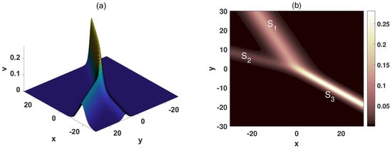
Figure 3. (a) The spatial structure of the Y-shaped soliton at $t=0$. (b) The density figure of (a).

Table 2. Physical quantities of the Y-shaped soliton arms.

Soliton	Trajectory	Velocity	Amplitude	Component
$S_1$	${\eta }_1=0$	$\left({\omega }_1,{\displaystyle \frac{{\omega }_1}{p_1}}\right)$	${\displaystyle \frac{k_1^2}{2}}$	$v_1$
$S_2$	${\eta }_2=0$	$\left({\omega }_2,{\displaystyle \frac{{\omega }_2}{p_2}}\right)$	${\displaystyle \frac{k_2^2}{2}}$	$v_2$
$S_3$	${\eta }_1-{\eta }_2=0$	$\left({\displaystyle \frac{k_1{\omega }_1-k_2{\omega }_2}{k_1-k_2}},{\displaystyle \frac{k_1{\omega }_1-k_2{\omega }_2}{k_1{p}_1-k_2{p}_2}}\right)$	${\displaystyle \frac{{(k1-k_2)}^2}{2}}$	$v_3$

3. Interaction Among Breather Wave, Transformed Wave and Soliton of the (2+1)-Dimensional pKP-BKP Equation

In this section, we investigate the interaction solutions based on the multi-soliton solution. For $N=3$ in Equation (3), the function f becomes:

$$\begin{array}{ccc}\hfill & & f_3=1-{\lambda }_{1}exp\left({\xi }_1\right)cos\left({\tau }_1\right)+{\displaystyle \frac{{\lambda }_1^2{H}_1}{4}}exp\left(2{\xi }_1\right)+{\displaystyle \frac{{\lambda }_1^2{H}_1}{4}}(H_{1r}^2+H_{1i}^2)exp\left(2{\xi }_1\right)\hfill \\ & & +exp\left({\eta }_3\right)\left(1+{\lambda }_{1}exp\left({\xi }_1\right)(H_{1r}cos\left({\tau }_1\right)-H_{1i}sin\left({\tau }_1\right))\right),\hfill \end{array}$$

(16)

with the complex conjugation limits for parameters as:

$$\begin{array}{ccc}& & k_1=a_1+b_{1}I=k_2^{*},p_1=c_1+d_{1}I=p_2^{*},{\varphi }_1=ln({\displaystyle \frac{{\lambda }_1}{2}})+{\delta }_1+{\gamma }_{1}I={\varphi }_2^{*},\hfill \\ & & k_3=k_3,p_3=p_3,{\varphi }_3={\varphi }_3,H_{1r}=Re(exp\left(A_{13}\right)),H_{1i}=Im(exp\left(A_{13}\right)).\hfill \end{array}$$

(17)

The transformed waves can be constructed by adjusting two characteristic lines as $L_{11}//L_{12}$:

$$\begin{array}{ccc}& & L_{11}:{\xi }_1+{\displaystyle \frac{{\lambda }_1}{2}}ln{H}_1=0,\hfill \\ & & L_{12}:{\tau }_1=0,\hfill \end{array}$$

with

$$\begin{array}{ccc}& & {\xi }_1=a_{1}x+(a_1{c}_1-b_1{d}_1)y+(a_1{M}_1-b_1{N}_1)t+{\delta }_1,\hfill \\ & & {\tau }_1=b_{1}x+(a_1{d}_1+b_1{c}_1)y+(a_1{N}_1+b_1{M}_1)t+{\gamma }_1,\hfill \\ & & H_1={\displaystyle \frac{15{\alpha }_1{b}_1^4-3(c_1{\alpha }_3+{\alpha }_2)b_1^2+{\alpha }_6{d}_1^2-5{\alpha }_1{a}_1^2{b}_1^2-{\alpha }_3{a}_1{b}_1{d}_1}{15{\alpha }_1{a}_1^4+3(c_1{\alpha }_3+{\alpha }_2)a_1^2+{\alpha }_6{d}_1^2-5{\alpha }_1{a}_1^2{b}_1^2-{\alpha }_3{a}_1{b}_1{d}_1}}>0,\hfill \\ & & M_1={\displaystyle \frac{(6a_1^2{b}_1^2-a_1^4-b_1^4){\alpha }_1-(a_1^2-b_1^2){\alpha }_2+c_1(2a_1{b}_1+b_1^2-a_1^2){\alpha }_3-{\alpha }_4-(c_1^2-d_1^2){\alpha }_6}{{\alpha }_5}},\hfill \\ & & N_1={\displaystyle \frac{-4a_1{b}_1(a_1^2-b_1^2){\alpha }_1-2a_1{b}_1{\alpha }_2+(-a_1^2{d}_1-2a_1{b}_1{c}_1+b_1^2{d}_1){\alpha }_3-2c_1{d}_1{\alpha }_6}{{\alpha }_5}}.\hfill \end{array}$$

The interactions between transformed waves and solitons are presented in Figure 4a–e. Figure 4a–c depict the interaction between a quasi-soliton and a soliton at different moments. A quasi-soliton and a soliton remain parallel during their propagation, traveling along the line $y={\displaystyle \frac{5}{14}}x$. It can be observed that the quasi-soliton moves faster than the soliton. The quasi-soliton continuously approaches the soliton and eventually overtakes it. The interactions between a multi-peak soliton/M-shaped soliton and a soliton are shown in Figure 4d and Figure 4e, respectively. With the condition Equation (13), the interaction between a Y-shaped soliton and a soliton is obtained (Figure 4f).

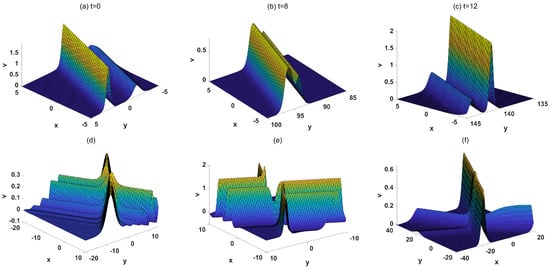
Figure 4. (a–c) The spatial structure of the interaction between a quasi-soliton and a soliton at different times. The parameters are chosen as ${\alpha }_1=-2,{\alpha }_2=1,{\alpha }_3=\sqrt{10},{\alpha }_4=1,{\alpha }_5=0.5$, ${\alpha }_6=1$, $a_1=1,b_1=0.2,c_1=2.8,k_3=3,p_3=2.8,{\delta }_1=0,{\gamma }_1=0,{\varphi }_3=10.$ (d) The spatial structure of the interaction between a multi-peak soliton and a soliton at $t=0$. The parameters are chosen as ${\alpha }_1=-2,{\alpha }_2=1,{\alpha }_3=\sqrt{10},{\alpha }_4=1,{\alpha }_5=0.5,{\alpha }_6=1,a_1=0.2,b_1=1,$ $c_1=-1.5$, $k_3=0.8,p_3=1,{\delta }_1=0,{\gamma }_1=0,{\varphi }_3=0.$ (e) The spatial structure of the interaction between an M-shaped soliton and a soliton at $t=0$. The parameters are chosen as ${\alpha }_1=-2,{\alpha }_2=1,{\alpha }_3=\sqrt{10}$, ${\alpha }_4=1$, ${\alpha }_5=0.5,{\alpha }_6=1,a_1=1,b_1=1,c_1=-0.5,k_3=-1.8,p_3=2,{\delta }_1=0,{\gamma }_1=0$, ${\varphi }_3=0.$ (f) The spatial structure of the interaction between a Y-shaped soliton and a soliton at $t=0$. The parameters are chosen as ${\alpha }_1=-1,{\alpha }_2=1,{\alpha }_3=5,{\alpha }_4=2,{\alpha }_5=1,{\alpha }_6=1,k_1=0.5$, $p_1=0.6$, $k_2=-0.25,p_2={\displaystyle \frac{39}{40}}+{\displaystyle \frac{3\sqrt{885}}{80}},k_3=1.1,p_3=-0.5,{\varphi }_1=0,{\varphi }_2=0,{\varphi }_3=10$.

In addition, the field $f_3$ can be rewritten as follows using the long wave limit method:

$$\begin{array}{ccc}& & f_3\sim (1+{\widehat{\xi }}_1^2+{\widehat{\tau }}_1^2){ϵ}^2+exp\left({\eta }_3\right)((1-2H_{1r}+H_{1r}^2+H_{1i}^2)+(-{\widehat{\xi }}_1+2H_{1i}{\widehat{\tau }}_1+{\widehat{\xi }}_1(H_{1r}^2+H_{1i}^2)ϵ)\hfill \\ & & +({\displaystyle \frac{1}{2}}{\widehat{\xi }}_1+H_{1r}{\widehat{\tau }}_1^2+({\displaystyle \frac{1}{2}}{\widehat{\xi }}_1+1)(H_{1r}^2+H_{1i}^2)){ϵ}^2)+O\left({ϵ}^3\right).\hfill \end{array}$$

(18)

As shown in Figure 5, the amplitude of the W-shaped soliton changes before and after the collision, while the amplitude of the soliton remains unchanged. The variation in peak heights reflects the exchange energy among the internal modes of the W-shaped wave during interaction. This modulation is a hallmark of higher-order nonlinear structures, where multiple localized peaks can absorb and release energy in a coordinated manner by the external solitary disturbance.

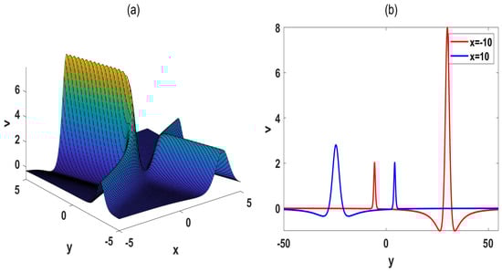
Figure 5. (a) The spatial structure of interaction between W-shaped soliton and soliton. The parameters are chosen as ${\alpha }_1=-2,{\alpha }_2=1,{\alpha }_3=\sqrt{10},{\alpha }_4=1,{\alpha }_5=0.5,{\alpha }_6=1,d_1=0,{\delta }_1=0,{\gamma }_1=0.$ (b) The cross-sectional graphs of (a).

Setting $N=4$ in Equation (3), the form of $f_4$ is as follows:

$$\begin{array}{ccc}\hfill & & f_4=1+{\lambda }_{1}exp\left({\xi }_1\right)cos\left({\tau }_1\right)+{\displaystyle \frac{{\lambda }_1^2{H}_1}{4}}exp\left(2{\xi }_1\right)+{\lambda }_{3}exp\left({\xi }_2\right)cos\left({\tau }_2\right)+{\displaystyle \frac{{\lambda }_3^2{H}_2}{4}}exp\left(2{\xi }_2\right)\hfill \\ & & +{\displaystyle \frac{{\lambda }_1^2{\lambda }_3{H}_1}{4}}exp(2{\xi }_1+{\xi }_2)((H_{1r}{H}_{2r}+H_{1i}{H}_{2i})cos\left({\tau }_2\right)-(H_{1i}{H}_{2r}-H_{1r}{H}_{2i})sin\left({\tau }_2\right))\hfill \\ & & +{\displaystyle \frac{{\lambda }_1{\lambda }_3^2{H}_2}{4}}exp({\xi }_1+2{\xi }_2)((H_{1r}{H}_{2r}-H_{1i}{H}_{2i})cos\left({\tau }_1\right)-(H_{1i}{H}_{2r}+H_{1r}{H}_{2i})sin\left({\tau }_1\right))\hfill \\ & & +{\displaystyle \frac{{\lambda }_1{\lambda }_3}{2}}exp({\xi }_1+{\xi }_2)(H_{1r}cos({\tau }_1+{\tau }_2)-H_{1i}sin({\tau }_1+{\tau }_2))\hfill \\ & & +{\displaystyle \frac{{\lambda }_1{\lambda }_3}{2}}exp({\xi }_1+{\xi }_2)(H_{2r}cos({\tau }_1-{\tau }_2)-H_{2i}sin({\tau }_1-{\tau }_2))\hfill \\ & & +{\displaystyle \frac{{\lambda }_1^2{\lambda }_3^2{H}_1{H}_2}{16}}exp(2{\xi }_1+2{\xi }_2)(H_{1r}^2+H_{1i}^2)(H_{2r}^2+H_{2i}^2),\hfill \end{array}$$

(19)

with

$$\begin{array}{ccc}& & k_3=a_2+b_{2}I=k_4^{*},p_3=c_2+d_{2}I=p_4^{*},{\varphi }_3=ln({\displaystyle \frac{{\lambda }_3}{2}})+{\delta }_2+{\gamma }_{2}I={\varphi }_4^{*},\hfill \\ & & H_{2r}=Re\left(exp\left(A_{14}\right)\right),H_{2i}=Im\left(exp\left(A_{14}\right)\right),\hfill \\ & & H_2={\displaystyle \frac{15{\alpha }_1{b}_2^4-3(c_2{\alpha }_3+{\alpha }_2)b_2^2+{\alpha }_6{d}_2^2-5{\alpha }_1{a}_2^2{b}_2^2-{\alpha }_3{a}_2{b}_2{d}_2}{15{\alpha }_1{a}_2^4+3(c_2{\alpha }_3+{\alpha }_2)a_2^2+{\alpha }_6{d}_2^2-5{\alpha }_1{a}_2^2{b}_2^2-{\alpha }_3{a}_2{b}_2{d}_2}}>0,\hfill \\ & & M_2={\displaystyle \frac{(6a_2^2{b}_2^2-a_2^4-b_2^4){\alpha }_1-(a_2^2-b_2^2){\alpha }_2+c_2(2a_2{b}_2+b_2^2-a_2^2){\alpha }_3-{\alpha }_4-(c_2^2-d_2^2){\alpha }_6}{{\alpha }_5}},\hfill \\ & & N_2={\displaystyle \frac{-4a_2{b}_2(a_2^2-b_2^2){\alpha }_1-2a_2{b}_2{\alpha }_2+(-a_2^2{d}_2-2a_2{b}_2{c}_2+b_2^2{d}_2){\alpha }_3-2c_2{d}_2{\alpha }_6}{{\alpha }_5}}.\hfill \end{array}$$

Under the condition $d_1=0$, the interaction between a quasi-soliton and a breather wave is shown in Figure 6a.

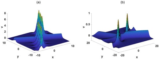
Figure 6. (a) The spatial structure of interaction between quasi soliton and breather wave at $t=0$. The parameters are chosen as ${\alpha }_1=-1,{\alpha }_2=1,{\alpha }_3=2,{\alpha }_4=1,{\alpha }_5=1,{\alpha }_6=0.8,a_1=1$, $b_1=0.2$, $c_1=1.95,d_1=0,{\delta }_1=0,{\gamma }_1=0,a_2=1,b_2=1,c_2=0.5,d_2=1,{\delta }_2=0,{\gamma }_2=0.$ (b) The spatial structure of interaction between Y-shaped soliton and breather wave at $t=0$. The parameters are choosed as ${\alpha }_1=-1,{\alpha }_2=1,{\alpha }_3=2,{\alpha }_4=1,{\alpha }_5=1,{\alpha }_6=0.8,a_1={\displaystyle \frac{1}{3}},b_1={\displaystyle \frac{1}{3}},c_1=-0.8$, $d_1=1$, ${\delta }_1=0,{\gamma }_1=0,k_3=0.5,k_4=-0.25,p_3=0.6,p_4={\displaystyle \frac{123}{80}}+{\displaystyle \frac{3\sqrt{453}}{32}},{\varphi }_3=0,{\varphi }_4=0$.

The interaction between a Y-shaped soliton and a breather wave can be constructed with Equation (13) and

$$\begin{array}{cc}{f}_4=\hfill & 1+exp\left({\eta }_1\right)+exp\left({\eta }_2\right)+exp\left({\eta }_3\right)+exp\left({\eta }_4\right)+A_{13}exp({\eta }_1+{\eta }_3)+A_{14}exp({\eta }_1+{\eta }_4)\hfill \\ \hfill & +A_{23}exp({\eta }_2+{\eta }_3)+A_{24}exp({\eta }_2+{\eta }_4)+A_{34}exp({\eta }_3+{\eta }_4)\hfill \\ \hfill & +A_{13}{A}_{14}{A}_{34}exp({\eta }_1+{\eta }_3+{\eta }_4)+A_{23}{A}_{24}{A}_{34}exp({\eta }_2+{\eta }_3+{\eta }_4).\hfill \end{array}$$

(20)

The corresponding three-dimensional plot is presented in Figure 6b. Figure 6 demonstrates that the collision affects only the phase of the wave.

4. Transformed Wave-Soliton Molecule and Transformed Wave Molecule of the (2+1)-Dimensional pKP-BKP Equation

A soliton molecule is a bound-state structure composed of two solitons with identical velocities. Soliton molecules have been experimentally observed, and the velocity resonance method provides an effective theoretical approach for obtaining such soliton molecules. In this section, the velocity resonance method is employed to obtain novel bound-state structures, such as the transformed wave–soliton, transformed wave-breather, and transformed wave molecules.

Case 1. A molecule composed of a transformed wave and a soliton for Equation (16) needs to satisfy:

$$\begin{array}{c}\hfill L_{11}//L_s,v_{1x}^s={\omega }_3,v_{1y}^s={\displaystyle \frac{{\omega }_3}{p_3}},\end{array}$$

(21)

with

$$\begin{array}{c}\hfill d_1=0,L_s:{\xi }_3=0.\end{array}$$

(22)

The molecule composed of M-shaped soliton and a soliton is presented in Figure 7. The corresponding parameters are:

$$\begin{array}{ccc}& & {\alpha }_1=-1,{\alpha }_2=1,{\alpha }_3=1,{\alpha }_4=1,{\alpha }_5=1,{\alpha }_6=0.2,{\varphi }_1=5,\hfill \\ & & a_1=1,b_1=1,c_1=1,k_3=\sqrt{2},p_3=1,{\delta }_1=-5,{\gamma }_1=0.\hfill \end{array}$$

The transformed wave and the soliton in Figure 7a–c propagate parallel to each other but at different speeds, resulting in collisions and changing their relative positions. The molecule depicted in Figure 7 maintains the same relative position throughout their propagation.

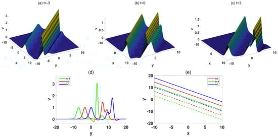
Figure 7. (a–c) The spatial structure of the molecule consisted of M-shaped soliton and soliton at $t=-3,t=0,t=3$, respectively. (d) The cross-sectional graphs of (a–c). (e) The characteristic lines of M-shaped soliton and the single soliton.

Case 2. As a four-soliton solution, Equation (19), under the following conditions:

$$\begin{array}{c}\hfill L_{11}//L_{21},\sqrt{{v_{1x}^s}^2+{v_{1y}^s}^2}=\sqrt{{v_{2x}^s}^2+{v_{2y}^s}^2},\end{array}$$

(23)

with

$$\begin{array}{ccc}& & L_{11}:{\xi }_1+ln({\displaystyle \frac{{\lambda }_1{H}_1}{2}})=0,\hfill \\ & & L_{21}:{\xi }_2+ln({\displaystyle \frac{{\lambda }_3{H}_2}{2}})=0,\hfill \end{array}$$

(24)

$d_1=0$ and selecting appropriate parameters:

$$\begin{array}{ccc}& & {\alpha }_1=-1,{\alpha }_2=1,{\alpha }_3=2,{\alpha }_4=1,{\alpha }_5=1,{\alpha }_6=0.8,a_1=0.99,b_1=1,\hfill \\ & & c_1=0.5,{\delta }_1=-1,{\gamma }_1=0,a_2=0.7,b_2=0,c_2=0.5,d_2=1,{\delta }_2=5,{\gamma }_2=0,\hfill \end{array}$$

the molecule consisting of an M-shaped soliton and a breather wave is plotted in Figure 8.

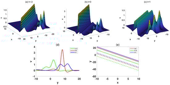
Figure 8. (a–c) The spatial structure of the M-shaped soliton-breather molecule at $t=-3,t=0,t=1$, respectively. (d) The cross-sectional graphs of (a–c). (e) The characteristic lines of the M-shaped solitin and one breather wave.

Case 3. Based on the above condition Equation (23) with $d_1=0$, $d_2=0$, and the parameters as:

$$\begin{array}{ccc}& & {\alpha }_1=-1,{\alpha }_2=1,{\alpha }_3=2,{\alpha }_4=1,{\alpha }_5=1,{\alpha }_6=0.8,a_1=1,b_1=1,\hfill \\ & & c_1=0.5,{\delta }_1=-1,{\gamma }_1=0,a_2=0.88,b_2=0.8,c_2=0.5,{\delta }_2=5,{\gamma }_2=0,\hfill \end{array}$$

the transformed molecule consisting of two transformed waves is shown in Figure 9.

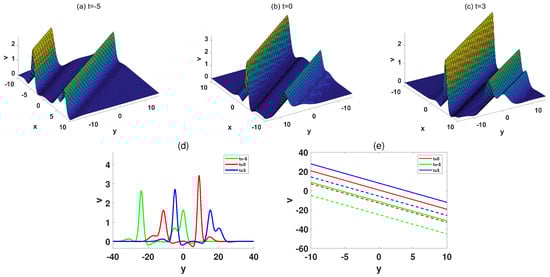
Figure 9. (a–c) The spatial structure of the soliton molecule consisted by two M-shaped solitons at $t=-5,t=0,t=3$, respectively. (d) The cross-sectional graphs of (a–c). (e) The characteristic lines of two M-shaped solitons.

From Figure 7d, Figure 8d and Figure 9d, it can be concluded that the transformed waves exhibit significant time-varying characteristics. It is worth noting that the two peak values of one of the transformed waves exchanged sizes. The left peak changed from low to high, and the right peak changed from high to low, as shown in Figure 9d. These molecule-type structures remain bound because the interacting waves share identical velocities under the resonance conditions. This velocity matching allows the waves to trap energy each other, producing a stable composite object. The amplitude exchange observed in the cross-sections reflects internal energy oscillation within the molecule, analogous to bonding dynamics in optical soliton molecules.

5. Conclusions

In this work, we have systematically investigated various nonlinear wave structures and interaction dynamics arising from the (2+1)-dimensional potential Kadomtsev–Petviashvili-B-type Kadomtsev–Petviashvili equation. Based on multi-soliton solutions derived via the Hirota’s bilinear method, we first explored resonance solitons including X-shaped and Y-shaped configurations, identifying the localized stem structures induced by infinite phase shifts. Detailed expressions for the trajectories, amplitudes, and velocities of soliton arms were provided, and it was found that the stem length remains invariant during propagation.

We presented various interaction scenarios among solitons, breathers, and transformed waves, revealing elastic features, including phase shifts and waveform modulation. Finally, several types of nonlinear wave molecules were constructed by imposing velocity resonance conditions. These localized waves include soliton-transformed wave molecules and transformed wave molecules, which exhibit novel dynamic features such as amplitude exchange and breath-type modulation. The rich structures uncovered in this study not only deepen our understanding of nonlinear wave dynamics in higher-dimensional integrable systems but also offer potential guidance for experimental exploration, particularly in fluid dynamics.

References

- Wang, Q.; Mihalache, D.; Belić, M.R.; Lin, J. Mode conversion of various solitons in parabolic and cross-phase potential wells. Opt. Lett. 2024, 49, 1607–1610. [Google Scholar] [CrossRef]
- Yao, X.M.; Zhao, J.F.; Liang, R. State-transition mechanisms for (2+1)-dimensional Sawada-Kotera equation with the variable coefficients in plasma physics and fluid dynamics. Chaos Solitons Fractals 2025, 197, 116485. [Google Scholar] [CrossRef]
- Wang, Q.; Mihalache, D.; Belić, M.R.; Zeng, L.; Lin, J. Spiraling Laguerre-Gaussian solitons and arrays in parabolic potential wells. Opt. Lett. 2023, 48, 4233–4236. [Google Scholar] [CrossRef]
- Mohan, B.; Kumar, S. Generalization and analytic exploration of soliton solutions for nonlinear evolution equations via a novel symbolic approach in fluids and nonlinear sciences. Chin. J. Phys. 2024, 92, 10–21. [Google Scholar] [CrossRef]
- Tanwar, D.V. Lie symmetry reductions and generalized exact solutions of Date-Jimbo Kashiwara-Miwa equation. Chaos Soliton Fractals 2022, 162, 112414. [Google Scholar] [CrossRef]
- Ablowitz, M.J.; Kaup, D.J.; Newell, A.C.; Segur, H. The inverse scattering transform-Fourier analysis for nonlinear problems. Stud. Appl. Math. 1974, 53, 249–315. [Google Scholar] [CrossRef]
- Satsuma, J. Hirota bilinear method for nonlinear evolution equations. In Direct and Inverse Methods in Nonlinear Evolution Equations; Springer: Berlin/Heidelberg, Germany, 2003; Volume 632, pp. 171–222. [Google Scholar]
- Kumar, S.; Kumar, A. Lie symmetry reductions and group invariant solutions of (2+1)-dimensional modified veronese web equation. Nonlinear Dyn. 2019, 98, 1891–1903. [Google Scholar] [CrossRef]
- Gu, C.H.; Hu, H.S.; Zhou, Z.S. Darboux Transformations in Integrable Systems: Theory and Their Applications to Geometry; Springer Science & Business Media: Berlin/Heidelberg, Germany, 2004. [Google Scholar]
- Taha, T.R.; Ablowitz, M.I. Analytical and numerical aspects of certain nonlinear evolution equations. II. Numerical, nonlinear Schrödinger equation. J. Comput. Phys. 1984, 55, 203–230. [Google Scholar] [CrossRef]
- Ma, W.X. Wronskians, generalized Wronskians and solutions to the Korteweg-de Vries equation. Chaos Solitons Fractals 2004, 19, 163–170. [Google Scholar] [CrossRef]
- Maccari, A. The Kadomtsev-Petviashvili equation as a source of integrable model equations. J. Math. Phys. 1996, 37, 6207–6212. [Google Scholar] [CrossRef]
- Pava, J.A.; Plaza, R.G. Instability theory of kink and anti-kink profiles for the sine-Gordon equation on Josephson tricrystal boundaries. Physica D 2021, 427, 133020. [Google Scholar] [CrossRef]
- Yang, Z.P.; Zhong, W.P. Dark Localized Waves in Shallow Waters: Analysis within an Extended Boussinesq System. Chin. Phys. Lett. 2024, 41, 044201. [Google Scholar] [CrossRef]
- Kath, W.L.; Smyth, N.F. Soliton evolution and radiation loss for the Korteweg-de Vries equation. Phys. Rev. E 1995, 51, 661. [Google Scholar] [CrossRef] [PubMed]
- Wang, L.H.; Porsezian, K.; He, J.S. Breather and rogue wave solutions of a generalized nonlinear Schrödinger equation. Phys. Rev. E 2013, 87, 053202. [Google Scholar] [CrossRef]
- Ma, W.X. Lump solutions to the Kadomtsev-Petviashvili equation. Phys. Lett. A 2015, 379, 1975–1978. [Google Scholar] [CrossRef]
- Kako, F.; Yajima, N. Interaction of ion-acoustic solitons in two-dimensional space. J. Phys. Soc. Jpn. 1980, 49, 2063–2071. [Google Scholar] [CrossRef]
- Ohkuma, K.; Wadati, M. The Kadomtsev-Petviashvili equation: The trace method and the soliton resonances. J. Phys. Soc. Jpn. 1983, 52, 749–760. [Google Scholar] [CrossRef]
- Shen, Y.; Tian, B.; Zhou, T.Y.; Gao, X.T. Shallow-water-wave studies on a (2+1)-dimensional Hirota-Satsuma-Ito system: X-type soliton, resonant Y-type soliton and hybrid solutions. Chaos Solitons Fractals 2022, 157, 111861. [Google Scholar] [CrossRef]
- Ablowitz, M.J.; Baldwin, D.E. Nonlinear shallow ocean-wave soliton interactions on flat beaches. Phys. Rev. E 2012, 86, 036305. [Google Scholar] [CrossRef]
- Chowdury, A.; Krolikowski, W. Breather-to-soliton transformation rules in the hierarchy of nonlinear Schrödinger equations. Phys. Rev. E 2017, 95, 062226. [Google Scholar] [CrossRef]
- Wang, L.; Zhang, J.-H.; Wang, Z.-Q.; Liu, C.; Li, M.; Qi, F.-H.; Guo, R. Breather-to-soliton transitions, nonlinear wave interactions, and modulational instability in a higher-order generalized nonlinear Schrödinger equation. Phys. Rev. E 2016, 93, 012214. [Google Scholar] [CrossRef] [PubMed]
- Chowdury, A.; Kedziora, D.J.; Ankiewicz, A.; Akhmediev, N. Breather-to-soliton conversions described by the quintic equation of the nonlinear Schrödinger hierarchy. Phys. Rev. E 2015, 91, 032928. [Google Scholar] [CrossRef] [PubMed]
- Huang, Q.M.; Gao, Y.T.; Hu, L. Breather-to-soliton transition for a sixth-order nonlinear Schrödinger equation in an optical fiber. Appl. Math. Lett. 2018, 75, 135–140. [Google Scholar] [CrossRef]
- Zhang, X.; Wang, L.; Liu, C.; Li, M.; Zhao, Y.-C. High-dimensional nonlinear wave transitions and their mechanisms. Chaos 2020, 30, 113107. [Google Scholar] [CrossRef]
- Zhang, X.Q.; Ren, B. Nonlinear waves and transition mechanisms for (2+1)-dimensional Korteweg-de Vries-Sawada-Kotera-Ramani equation. Wave Motion 2024, 130, 103383. [Google Scholar] [CrossRef]
- Ma, Y.L.; Li, B.Q. Soliton interactions, soliton bifurcations and molecules, breather molecules, breather-to-soliton transitions, and conservation laws for a nonlinear (3+1)-dimensional shallow water wave equation. Nonlinear Dyn. 2024, 112, 2851–2867. [Google Scholar] [CrossRef]
- Zhang, X.Q.; Ren, B. Conversion mechanisms and transformed waves for the (3+1)-dimensional nonlinear equation. Phys. Fluids 2024, 36, 102129. [Google Scholar] [CrossRef]
- Krupa, K.; Nithyanandan, K.; Andral, U.; Tchofo-Dinda, P.; Grelu, P. Real-time observation of internal motion within ultrafast dissipative optical soliton molecules. Phys. Rev. Lett. 2017, 118, 243901. [Google Scholar] [CrossRef]
- Stratmann, M.; Pagel, T.; Mitschke, F. Experimental observation of temporal soliton molecules. Phys. Rev. Lett. 2005, 95, 143902. [Google Scholar] [CrossRef]
- Herink, G.; Kurtz, F.; Jalali, B.; Solli, D.R.; Ropers, C. Real-time spectral interferometry probes the internal dynamics of femtosecond soliton molecules. Science 2017, 356, 50–54. [Google Scholar] [CrossRef]
- Li, B.M. Optical soliton resonances and soliton molecules for the Lakshmanan-Porsezian-Daniel system in nonlinear optics. Nonlinear Dyn. 2023, 111, 6689–6699. [Google Scholar] [CrossRef]
- Lou, S.Y. Soliton molecules and asymmetric solitons in three fifth order systems via velocity resonance. J. Phys. Commun. 2020, 4, 041002. [Google Scholar] [CrossRef]
- Ma, Y.X. Soliton resonances, soliton molecules, soliton oscillations and heterotypic solitons for the nonlinear Maccari system. Nonlinear Dyn. 2023, 111, 18331–18344. [Google Scholar] [CrossRef]
- Ma, W.X. N-soliton solution of a combined pKP-BKP equation. J. Geom. Phys. 2021, 165, 104191. [Google Scholar] [CrossRef]
- Ma, H.C.; Yue, S.P.; Deng, A.P. Lump and interaction solutions for a (2+1)-dimensional combined pKP-BKP equation in fluids. Mod. Phys. Lett. B 2022, 36, 2250069. [Google Scholar] [CrossRef]
- Ma, H.C. Complexiton solutions, kink soliton and breather-wave solutions for the (2+1)-dimensional combined potential Kadomtsev-Petviashvili with B-type Kadomtsev-Petviashvili equation. Phys. Scr. 2023, 98, 095239. [Google Scholar] [CrossRef]
- Zhang, L.H.; Zhao, Z.L.; Zhang, Y.F. Dynamics of transformed nonlinear waves for the (2+1)-dimensional pKP-BKP equation: Interactions and molecular waves. Phys. Scr. 2024, 99, 075220. [Google Scholar] [CrossRef]
- Feng, Y.; Bilige, S. Resonant multi-soliton, M-breather, M-lump and hybrid solutions of a combined pKP-BKP equation. J. Geom. Phys. 2021, 169, 104322. [Google Scholar] [CrossRef]
- Tariq, K.U.; Wazwaz, A.M.; Tufail, R. Lump, periodic and travelling wave solutions to the (2+1)-dimensional pKP-BKP model. Eur. Phys. J. Plus 2022, 137, 1100. [Google Scholar] [CrossRef]
Disclaimer/Publisher’s Note: The statements, opinions and data contained in all publications are solely those of the individual author(s) and contributor(s) and not of MDPI and/or the editor(s). MDPI and/or the editor(s) disclaim responsibility for any injury to people or property resulting from any ideas, methods, instructions or products referred to in the content. |
© 2025 by the authors. Licensee MDPI, Basel, Switzerland. This article is an open access article distributed under the terms and conditions of the Creative Commons Attribution (CC BY) license (https://creativecommons.org/licenses/by/4.0/).