Abstract
This paper introduces the UG-EM (Unconditional Gamma-Exponential Model) as a new compound lifetime model designed to enhance flexibility in tail behavior compared to traditional distributions. The UG-EM model provides a unified framework for analyzing deviations from symmetry in survival data, effectively capturing right-skewed patterns, which are commonly observed in real-world lifetime phenomena. The main analytical properties are derived, including the probability density, cumulative distribution, hazard and reversed-hazard functions, mean residual life, and several measures of dispersion and uncertainty. The effects of the UG-EM parameters (α and λ) are examined, showing that increasing either parameter can cause a temporary reduction in entropy H(T) at early times followed by a long-term increase; in some cases, the influence of α is stronger than that of λ. Parameter estimation is carried out using the maximum likelihood method and assessed through Monte Carlo simulations to evaluate estimator bias and variability, highlighting the significant role of sample size in estimation accuracy. The proposed model is applied to three survival datasets (Lung, Veteran, and Kidney) and compared with classical alternatives such as Exponential, Weibull, and Log-normal distributions using standard goodness-of-fit criteria. Results indicate that the UG-EM model offers superior flexibility and can capture patterns that simpler models fail to represent, although the empirical results do not demonstrate a clear, consistent superiority over standard competitors across all tested datasets. The paper also discusses identifiability issues, estimation challenges, and practical implications for reliability and medical survival analysis. Recommendations for further theoretical development and broader model comparison are provided.
1. Introduction
Mixture models and unconditional distribution models have been widely applied in the analysis of lifetime and survival data, particularly for capturing unobserved heterogeneity.
Pickles in [1] reviewed some of the main approaches to the analysis of multivariate censored survival data. They compared the performance of conditional and mixture likelihood approaches in estimating models with frailty effects in censored bivariate survival data and found that the mixture methods were surprisingly robust against misspecification of the frailty distribution. Building on the idea of model flexibility, Ref. [2] proposed a generalized Weibull distribution (the exponentiated Weibull), providing greater flexibility in modeling various shapes of hazard functions (increasing, decreasing, and bathtub-shaped). Similarly, Ref. [3] developed a mixture model based on the extended exponential–geometric distribution to describe heterogeneous survival data, where the maximum likelihood method was used to estimate the model parameters. In contrast, Ref. [4] developed survival models derived from stable distributions of the positive numbers—the gamma, the degenerate, and the inverse Gaussian distributions—to describe heterogeneity in populations and to show how these models affect hazard and survival functions.
Lawless in [5] provides a comprehensive framework for modeling and analyzing lifetime data. The book covers classical lifetime distributions, such as Weibull, Exponential, and Gamma, along with methods for parameter estimation. In addition to that, Ref. [6] addresses censored and truncated data, life testing, hazard models, and diagnostic tools for assessing system performance based on empirical data.
Another important contribution to the field of reliability engineering emphasizing practical and lifetime modeling was made by [7], while Ref. [8] presented a mathematical and probabilistic treatment of lifetime distributions, including Weibull models and other theoretical aspects.
Kuo and Peng in [9] introduced a mixture model approach to analyze beetle data that included both exact observations and interval-censored cases. Building on this line of research, later contributions have sought to develop more flexible lifetime models. For instance, Rubio and Hong [10] proposed a log two-piece model as a flexible class of lifetime distribution. They estimated its parameters via maximum likelihood and evaluated the model using information criteria such as AIC. The applicability of their method was further demonstrated with real datasets, including Mayo primary biliary cirrhosis and lung cancer studies.
In addition to mixture and frailty approaches, considerable attention has been given to extending simple one-parameter models, such as exponential distribution, by additional parameters, often to provide greater flexibility in the tail behavior. Ref. [11] was among the first to formalize this idea, proposing the Beta-G family of distributions by embedding the Beta distribution to generate new probability models. This framework was subsequently broadened by [12], which developed the mathematical properties of these generated families, including their density and distribution functions, moments, and reliability characteristics.
Building on the work of Kumaraswamy, Cordeiro and de Castro, Ref. [13], introduced a new family of generalized distributions extending classical models such as the Weibull and Gamma. This idea was further developed through the generalized beta-generated family [14], enhancing flexibility in modeling hazard behaviors. Later, Torabi and Montazari [15] proposed the logistic-uniform distribution, adding additional adaptability to lifetime modeling. Collectively, these studies advanced the theoretical foundation for developing more flexible and realistic reliability models.
Many flexible lifetime models have been proposed by introducing extra shape parameters, compounding techniques, and hierarchical structures. Study [16] introduced the beta exponential distribution, an extension of the classical exponential model obtained by applying the beta generator to provide more flexibility in modeling lifetime data with various hazard rate shapes. The study provided a comprehensive treatment of the mathematical properties of the distribution. Similarly, Ref. [17] proposed a four-parameter lifetime model, called the gamma-extended Fréchet distribution, which is a new lifetime model that generalizes the traditional Fréchet distribution. Later, Ref. [18] developed a new general method for generating families of continuous distributions based on transformations of random variables. Collectively, these contributions have advanced the development of flexible distribution families for lifetime and reliability modeling.
Kundu and Gupta [19] investigated the Marshall–Olkin bivariate Weibull distribution, developed Bayesian estimation methods for its parameters, and provided a comprehensive framework for analyzing dependent lifetime data, enhancing reliability analysis in multicomponent systems. In contrast, Ref. [20] proposed a generalized modified Weibull distribution, extending the classical Weibull model to capture a wide variety of hazard rate shapes. These models are able to capture various hazard patterns, including bathtub-shaped, unimodal, and other non-monotonic forms often observed in reliability and medical data.
Ghitany, Atieh, and Nadarajah [21] examined the Lindley distribution as an alternative to the exponential model, complementing the exponential–geometric model earlier proposed by Adamidis and Loukas in 1998 and demonstrating its effectiveness for lifetime data with non-constant hazard rates. Study [22] introduced the complementary exponential–geometric distribution, further enhancing flexibility in modeling heterogeneous survival data. Complementing these distributional developments, Ref. [23] presented a comprehensive framework for Bayesian survival analysis, offering powerful inferential tools for lifetime modeling. Meanwhile, the book by Ref. [24] focused on the analysis of multivariate survival data, addressing dependence structures among correlated lifetimes. Its strong emphasis on conceptual foundations and modeling strategies makes it an equally valuable reference for both applied statisticians and practitioners.
Ref. [25] proposed a modified Weibull extension to model bathtub-shaped failure rates, addressing early failures, stable periods, and wear-out phases. Building on methodological developments in survival analysis, Ref. [26] provided tools for analyzing interval-censored failure time data. Extending previous ideas introduced by Lehmann in 1953, these were later applied by Refs. [16,27], who introduced a class of exponentiated generalized distributions, highlighting their properties and real-data applications. Similarly, Ref. [28] developed the beta generalized exponential distribution to flexibly model diverse lifetime behaviors. Ref. [29] presented the generalized additive models for location, scale, and shape, offering a flexible framework for modeling univariate response variables. Collectively, these studies enriched the statistical framework for analyzing complex survival and reliability data.
Building on the foundational distributional frameworks, recent studies have utilized established estimation and analytical techniques to investigate the properties of newly developed lifetime models. Ref. [30] proposed shrinkage-type estimators and compared them with the standard maximum likelihood estimation (MLE) method in reliability analysis. Ref. [31] examined the mathematical properties of two newly introduced lifetime distributions, deriving survival and hazard functions, moments, moment-generating functions, mean deviation, Rényi entropy, and quantile functions, and demonstrated the consistency of MLE through Monte Carlo simulations. Similarly, Refs. [32,33] introduced new families of compound probability distributions and analyzed their statistical characteristics using MLE. Ref. [34] derived analytical expressions for the PDF, CDF, survival, and hazard functions, mean residual life, and several entropy measures for an entropy-transformed Weibull model. Ref. [35] focused on cumulative residual entropy and its dynamics for residual lifetimes, while Ref. [36] examined generalized entropy measures to assess information loss in reliability systems. Expanding on these developments, Ref. [37] proposed extended concepts of cumulative residual entropy and formulated expressions for residual and cumulative entropies for continuous distributions. Collectively, these studies highlight how established statistical tools continue to enhance the analysis, characterization, and understanding of complex modern lifetime distributions.
Mixture models combine two or more probability distributions to represent heterogeneous populations. The mixed distribution describes the overall population, while the mixing distribution assigns weights to each component. Mathematically, it is expressed as , where denotes the mixture distribution, is the conditional (component) density function of given and is the mixing distribution, determining the relative contributions of each [38].
2. Model Formulation
2.1. Unconditional Model
Suppose T has a (conditional on
) Gamma distribution with mean
, and
has an exponential distribution with mean
. In this case the unconditional distribution of T is a mixture model which is called the Unconditional Gamma–Exponential Model (UG-EM).
Let the conditional (on ) probability density function of T be given by
With shape and rate . Suppose that itself follows an exponential distribution with rate :
The unconditional (marginal) distribution of T is
where and are the shape and scale parameters, respectively, of the disruption. Usually, is called mixed distribution, while is called mixing distribution. Now let us check , which is a probability density function.
2.2. Special Cases
- -
- In UG-EM, if ,
The Lomax (Pareto Type II) distribution is as follows:
Thus, when , the UG-EM density coincides with the Lomax (Pareto Type II) distribution. Lomax, in [39], introduced the Lomax distribution, also known as the Pareto Type II distribution, which is a two-parameter model widely used in reliability and economics.
The primary motivation for introducing the UG-EM model is its Compound Probabilistic Structure. It is explicitly derived as an Unconditional Gamma–Exponential (UG-EM) lifetime model, utilizing the Gamma–Exponential methodology to model Unobserved Heterogeneity. This provides a robust statistical framework for lifetime analysis. Furthermore, we note that the Lomax (or Pareto Type II) distribution is a two-parameter special case within the broader UG-EM family, occurring when ( = 1), but the UG-EM model operates on a broader parameter space ( > 0).
- -
- The (UG-EM), can be written as
If we put , we get
By comparison with Beata-prime distribution with , noting that , we get that UG-EM is a scaled version of the Beta-prime distribution with parameters .
We note that the analytical expression for the probability density function of the UG-EM model is algebraically equivalent to that of a scaled Beta-prime distribution in [40]. However, the derivation of these functions in this section serves a crucial methodological and analytical purpose.
2.3. Cumulative Distribution (CDF) of (UG-EM)
It is easy to check .
A graphical illustration is shown by
Figure 1, in which we present both the probability density function
and the cumulative distribution function
for several values of the parameters α and λ. This helps visualize the flexibility of the model and its ability to represent various types of lifetime data.
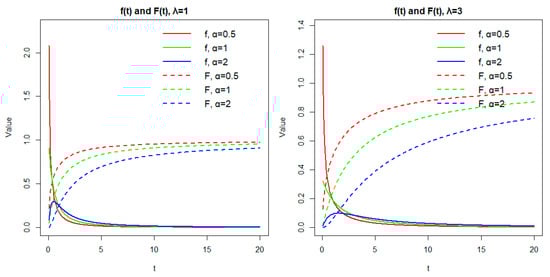
Figure 1.
Graphical illustration of and for several values of parameters.
3. Model Analysis: Reliability and Statistical Properties
3.1. Reliability and Hazard Rate Functions
The reliability function, denoted by R(t), measures the probability that a system or component will still operate without failure during a specified period of time t. The reliability function can be expressed as
Clearly,
- -
- Large , (high chance of failure)
- -
- Small , (high chance of survival)
The hazard rate function represents the instantaneous rate of occurrence of an event (such as failure or death) at a specific time t given that the event has not occurred up to that time. For a given distribution, is defined simply as
where and are the density and reliability functions for this distribution. Substituting the density and reliability functions of our model from Equations (3) and (6), for we get the following form:
It is clear that at , we get , representing a hyperbolic decline over time. This coincidence is unusual, since in general, and exhibit very different shapes.
The reliability function R(t) and hazard rate h(t) are used to describe the lifetime behavior of the proposed model, allowing us to analyze how the system’s survival probability and risk of failure evolve over time. Figure 2 illustrates and for different values of the parameters. Figure 3 illustrates the reliability function and hazard rate and how survival and risk evolve over time with different values of parameters α (shape parameter) and λ (scale parameter). The curve declines from unity toward zero, with a steeper descent when the shape parameter α exceeds unity. The hazard curve exhibits a decreasing profile over time for α below unity, remains flat when α equals unity, and rises when α exceeds unity.
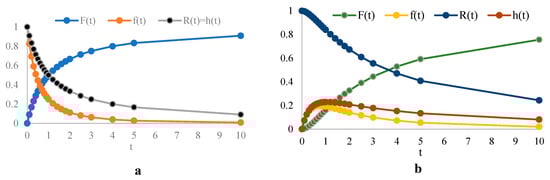
Figure 2.
and for different times with (a) and , (b) and .
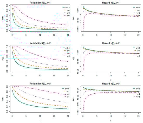
Figure 3.
Reliability and hazard functions for varying shape (α) and scale (λ) parameters.
3.2. Reversed Hazard Rate
The reversed hazard rate (RHR) is an important concept with diverse applications in actuarial sciences, forensic studies, and various other fields. The reversed hazard rate (RHR) describes the instantaneous failure rate at time , conditional on the event having occurred at or before t. Mathematically, it is defined as
where and F(t) are the probability density function (pdf) and cumulative distribution function (cdf) of the non-negative random variable T, respectively. In the UG-EM model, the RHR formula is obtained directly from the general definition:
which is decreasing over time. Figure 4 presents the pattern of r(t) and h(t) for different values of these parameters. Different curves illustrate how parameters such as or influence the failure dynamics. decreases initially, then may increase again, indicating changing survival behavior; however, increases, showing that the system becomes more likely to fail over time (aging effect). This contrast highlights that survival expectations and transient failure risk are not always moving in the same direction, and thus, it is important to take both roles into account when a general reliability estimate is needed. The hazard rate and the reversed hazard rate are complementary concepts, they provide a complete picture of the failure behavior of a system, capturing both future and past perspectives of risk.
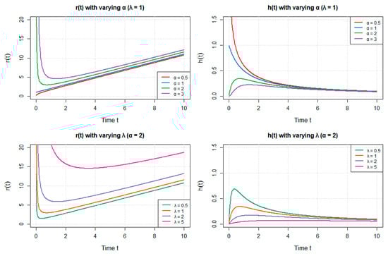
Figure 4.
Different curves of with of UG-EM for different values of parameters and .
3.3. Effect of Parameters
In the following, we present a graphical illustration of these parameters’ effects on reliability function , hazard rate and mean residual life
Figure 5 illustrates how the reliability function , hazard rate , and mean residual life vary with parameters α and λ. As shown, the system exhibits clear parametric sensitivity, with noticeable gradients in all three plots. In particular, the reliability decreases when increasing both parameters, while the hazard rate and residual life respond nonlinearly, indicating the complex behavior of the model under different parameter regimes.
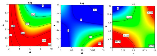
Figure 5.
Illustration of the effects of parameters α and λ on reliability function R(t), hazard rate h(t), and mean residual life r(t).
3.4. The Mean Residual Life (MRL)
The Mean Residual Life (MRL), which is also referred to as remaining lifetime, is a survival analysis concept. It tells us the expected time left until an event occurs, given that a system has survived up to a certain point. Mathematically, the mean residual life at time t, denoted as MRL(t), is defined as follows [41].
Let us use this idea of binomial expansion to clarify the discoveries of .
For large x, we have , and therefore
Similarly,
Hence, for sufficiently large
Thus,
So, diverges for any In the following, Table 1 presents the pattern of MRL for different values of parameters at fixed time.

Table 1.
The MRL of UG-EM at and , for different values of α and .
Clearly, MRL is increasing for the increasing. This is illustrated graphically in Figure 6.
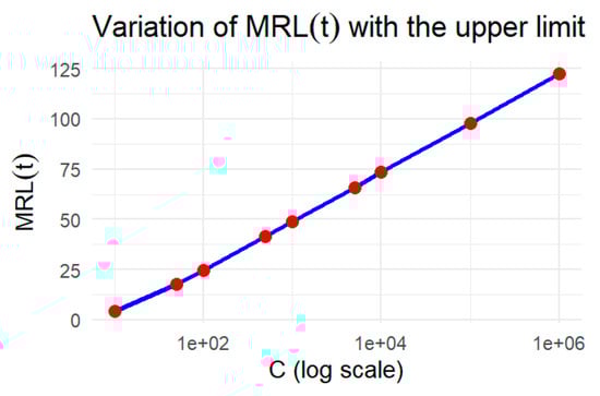
Figure 6.
The MRL of UG-EM with increasing values of C.
4. The Moments of UG-EM
This section focuses on the moments of the UG-EM distribution, which are key statistical measures used to describe its central tendency, variability, and shape.
4.1. The Moments
We analyzed the limit behavior of this integration as approaches infinity for ; regrettably, we found that the integral does not converge to a finite value. Let us see the mean
Lat then
where
Let split to be
where
Then, is finite. For , we have
So,
Therefore, and hence
And the variance
where
Similarly, by applying the same asymptotic argument to as for , we get , therefore .
In such cases, asymptotic analysis, numerical evaluation, or simulation-based approaches can be employed to provide clearer insights.
4.2. Simulation and Numerical Approximation
In this section, we present a numerical approximation of the integrals for , and as the upper limit c increases, for fixed values of the parameters α and λ. Table 2 presents numerical approximation for the behavior of the mean and variance of the UG-EM model at cutoff c. Also, graphical illustration is presented in Figure 7.
Table 2.
Approximate values of and for different values of α, λ, and cutoff c, based on numerical integration.
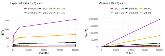
Figure 7.
Growth of and over time for the UG-EM model at different values of the model parameters.
Clearly, as the integration limit c increases, both E(T) and Var(T) are constantly increasing. In the limit as c→∞, the values approach their theoretical (possibly infinite) expectations.
The functions increase steadily with c, because the integrand is always positive, so adding more area as c grows naturally leads to a larger total value.
4.3. The Mode and the Median of UG-EM
- -
- The median is the solution of this equation
- -
- The mod of the UG-EM is that satisfies this equation
By solving this equation, we get
In the following, Table 3 presents numerical computations of the median and mode of the UG-EM model for different parameter values.
Table 3.
Median and mode of UG-EM for different values of its parameters.
Figure 8, below, presents how the parameters effect the patterns of the median and mode of the model.
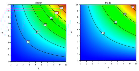
Figure 8.
Effect of both α and λ on the median and mode of the UG-EM.
5. Entropy
In information theory, entropy is a measure of the amount of information or uncertainty in a system. It is a non-negative measure, and it depends on the probability distribution of events or outcomes. High entropy means more randomness and unpredictability in the data, while low entropy implies more predictability and less information content and less surprise. It finds applications in diverse scientific and engineering contexts. The entropy of the random variable , with a density function , is defined as the expectation of the function
According to the UG-EM
Entropy shows how uncertain or spread out the outcomes behave, while expectation shows the average outcome in the center of the data. That is why putting them side by side in a table makes the analysis clearer and more insightful. In Table 4 and Figure 9, as follow, we present the expectation and entropy for the UG-EM model at different values of and .
Table 4.
Expectation and entropy evolution in UG-EM over time for varying α and λ.
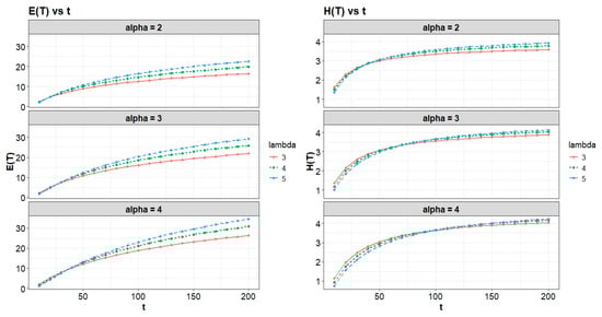
Figure 9.
Expectation and entropy evolution in UG-EM over time for varying α and λ.
Table 4 and Figure 9 illustrate the time evolution of the expectation and entropy for UG-EM for various values of α and λ. The two quantities increase with time, which means the system is developing and becoming more uncertain. Still, entropy grows more slowly. Changes in α affect the system much more strongly than changes in λ, something we will see more clearly below. These results are numerical approximations intended to illustrate how the system’s behavior changes with the parameters, even in cases where the theoretical integrals do not converge.
When fitting the data for E(T) and H(T) in Table 4, a quadratic model yields values of % and 98.9%, respectively. This indicates that both α and λ have a significant effect on increases or decreases in the system mean or entropy. Such influence reflects a higher degree of disorder and unpredictability within the UG-EM model. Figure 10 presents these effects.

Figure 10.
The effect of parameters and on E(T) and H(t) at a fixed time.
Clearly, E(T) increases with both α and λ. Conversely, H(T) exhibits a decreasing trend with increasing values of both parameters. These plots capture the behavior at a specific moment in time.
It is important to note, from Table 4 and Figure 10, that both the mean E(T) and entropy H(T) increase over time, indicating system growth and rising uncertainty. However, at fixed times there are small transient effects: increasing α or λ can produce a temporary concentration (slight decrease) in H(T) at early times, while their net effect over longer time horizons is an increase in H(T). The influence of α is stronger than that of λ.
6. Order Statistics
Consider an . random sample of size , denoted as , selected from a continuous distribution with probability density function and cumulative distribution function Let … , represent the corresponding order statistics. The probability density function (pdf) of the order statistic, denoted as , are given by [42]
and corresponding cumulative distribution function (cdf)
As a special case, we have
For, and .
Figure 10 below presents the PDF of the k-th order statistic for specific parameter values.
The plot in Figure 11
illustrates the behavior of the probability density functions (PDFs) of order statistics
from a UG-EM distribution for sample size
, with shape parameter
and rate parameter
. We see the peak of each curve move to the right and become lower as
k
increases. In plain terms: the smaller order statistics concentrate near low
t-values (the sample minimum), while the larger ones appear at higher t-values and are more spread out. These patterns match the usual behavior of ordered samples.
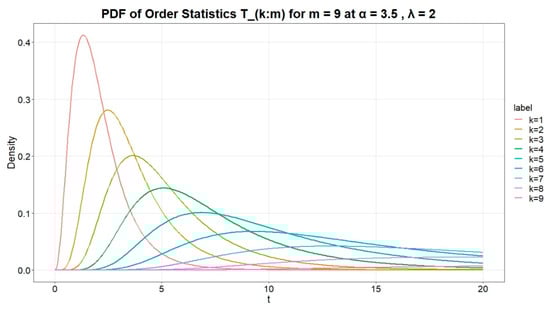
Figure 11.
Illustration of the probability density behavior of the k-th order statistics for a fixed sample size and fixed parameters.
7. Statistical Inference (Estimation)
7.1. Maximum Likelihood Estimation (MLE)
By maximizing the likelihood function (LF), we seek the parameter values that make the observed data most likely to occur. This approach ensures that our estimated model aligns well with the actual data we have at hand. We consider a random sample,
, drawn from the (UG-EM) in (1), with the following joint probability function (the likelihood function)
By taking the natural logarithm of the in Equation (21), we get
- -
- when is known, , the MLE of is simply the solution of the following differential equation
- -
- Similarly, when is known, , the MLE of is simply the solution of the following differential equation
- -
- When both α and λ are not known, in such a scenario the Maximum Likelihood Estimates (MLEs) for these parameters are the simultaneous solutions of the following system of equations
This system of nonlinear equations cannot be solved theoretically; therefore, it will be addressed numerically using an appropriate iterative method, such as the Newton–Raphson method or the Gradient Descent Optimization Method, which will be utilized later.
7.2. Fisher Information and Confidence Intervals
The inverse of the Fisher information matrix provides us with the asymptotic covariance matrix for the Maximum Likelihood Estimates (MLEs) of the parameters θ, where . This matrix is an important tool in statistical analysis because it describes how the uncertainties in the estimating process change as we gather more data or as our sample size increases, contributing valuable insights into the precision of our parameter estimates. In the following, the observed Fisher information matrix is presented
where is defined is Equation (22). In this case, the covariance matrix becomes simply . The approximate confidence limit (CLs) for the parameters are as follows:
respectively. Where and are the variances of and , respectively, which are calculated from the observed data and presented through the diagonal element of . Also, is the value corresponding to the upper percentile of the standard normal distribution.
7.3. Simulation
In the nonlinear system described by Equation (3), we generated 100 different samples from our model UG-EM using various assumed parameter values and and different sample sizes and Each case was repeated 100 times to obtain the empirical means, biases, and mean squared errors (MSE) of the estimators. In addition, bootstrap confidence intervals were computed at 90% and 95% levels to evaluate the precision and reliability of the estimates.
The simulation results in Table 5 show that the MLEs of the UG-EM parameters improve as the sample size increases. The bias and MSE decrease with larger samples, indicating consistency and convergence of the estimators toward the true parameter values and how the sample size greatly affects the estimation process. Moreover, the confidence intervals become narrower at higher sample sizes, confirming greater precision and reliability in the parameter estimation process. The QQ plots in Figure 12 further illustrate this behavior by comparing the sample quantiles of the simulated data with the corresponding theoretical quantiles of the UG-EM distribution for several values of α and λ at different sample sizes. As the sample size increases, the points align more closely with the 45° reference line, reflecting improved agreement between the simulated and theoretical distributions. The plots confirm that the UG-EM distribution fits the simulated data well and that larger samples provide more accurate representations of the theoretical distribution.
Table 5.
Estimation results for UG-EM parameters Θ = (α, λ): MLEs averages, biases, MSEs, and CIs for different sample sizes.
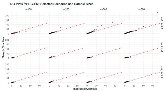
Figure 12.
QQ plots for the UG-EM distribution for selected parameter values (α and λ) across different sample sizes (n = 100, 200, 300, 500).
8. Application
The fitness of the UG-EM model can be demonstrated through its application to three well-known survival datasets available in the R survival package: first, Lung data, which is from a clinical trial of non-small cell lung cancer patients, from treatment initiation to death or last follow-up. This records the time of survival in days from treatment initiation to death or censoring. Then, Kidney data: This measurement records the time to graft failure in kidney transplant recipients from the surgery date to the date of failure or the end of observation. Finally, Veteran data: These were received in a trial comparing two therapies for small-cell lung cancer. The data estimate the time of survival in days from entry until censoring or death.
Note: It should be noted that the current analysis assumes complete observations. Right-censored data are not explicitly handled in this study, and the reported results should be interpreted accordingly. Future work will extend the model to properly account for censoring in survival datasets.
Data Sources and Ethical Statement: The datasets used in this study (Lung, Veteran, and Kidney) are publicly available through the R survival package (2025.09.0+387). All datasets are fully de-identified and therefore exempt from ethical approval. The Lung dataset originates from the North Central Cancer Treatment Group (NCCTG) study on prognostic variables in advanced lung cancer patients [43]. The Veteran dataset is based on the data described in Kalbfleisch and Prentice [44]. The Kidney dataset corresponds to catheter survival data analyzed using frailty models [45].
In Table 6 and according to the criteria AIC and BIC, the Weibull model is the best-fitting model for both Veteran and Lung datasets due to the minimum value of both of them, while the Log-normal distribution is a close second-best fit for both these datasets, particularly for the Veteran data. The Log-normal model gives the best fit for the Kidney data. The UG-EM model did not outperform other candidates in any of the datasets, although it showed competitive performance in the Kidney data. Notably, the Gamma model failed to fit the data well, so it was excluded from the final comparisons.
Table 6.
Comparison of exponential, Weibull, Log-normal, and UG-EM models on Lung, Veteran, and Kidney data.
The UG-EM model is particularly well-suited to capture the behavior of the data that has a long survival time and decays noticeably more slowly than an exponential curve. In other words, it has a heavy or slowly vanishing right tail.
In the following, a graphical comparison of the Exponential, Weibull, Log-normal, and UG-EM models based on Lung, Veteran, and Kidney data is presented in Figure 13.
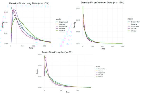
Figure 13.
Comparison of exponential, Weibull, Log-normal, and UG-EM Models on Lung, Veteran, and Kidney data.
9. Conclusions
We proposed the UG-EM (Unconditional Gamma–Exponential) model as a flexible compound lifetime distribution for analyzing right-skewed survival data. The study presents a complete analytical development, including density, cumulative, hazard, and reversed-hazard functions, along with measures of dispersion, entropy, and mean residual life. Simulation studies, including convergence diagnostics and bootstrap confidence intervals, confirmed the stability and consistency of the MLEs, especially for larger sample sizes. Applications to real datasets (Lung, Veteran, Kidney) showed that the model effectively captures deviations from symmetry and provides meaningful insights into parameter behavior. Overall, the UG-EM model offers a useful and analytically tractable framework for lifetime modeling, complementing existing distributions without claiming to universally outperform them. Future studies could extend the UG-EM distribution to more generalized forms, assess its performance on larger and more diverse datasets, and compare it with advanced survival models. Deeper mathematical investigation of its properties and evaluating its behavior under complex censoring schemes also represent promising directions for future research.
Author Contributions
Methodology, S.M.A.; Software, S.M.A.; Validation, O.H.O. and S.M.A.; Formal analysis, S.M.A.; Investigation, S.M.A.; Data curation, S.M.A.; Writing—original draft, O.H.O., S.M.A. and S.A.; Writing—review & editing, O.H.O., S.M.A. and S.A.; Visualization, S.M.A.; Supervision, S.M.A.; Project administration, S.M.A.; Funding acquisition, O.H.O. and S.A. All authors have read and agreed to the published version of the manuscript.
Funding
Princess Nourah bint Abdulrahman University Researchers Supporting Project number (PNURSP2025R743), Princess Nourah bint Abdulrahman University, Riyadh, Saudi Arabia.
Data Availability Statement
The original contributions presented in this study are included in the article. Further inquiries can be directed to the corresponding author.
Acknowledgments
The authors would like to extend their sincere appreciation to the Princess Nourah bint Abdulrahman University Researchers Supporting Project number (PNURSP2025R743), Princess Nourah bint Abdulrahman University, Riyadh, Saudi Arabia. Also, the authors would like to acknowledge the support of Prince Sultan University for their financial support.
Conflicts of Interest
The authors declare no conflicts of interest.
Abbreviations
| UG-EM | Unconditional Gamma-Exponential Model |
| HRF | Hazard rate function |
| RF | Reliability function |
| Sk | Coefficient of skewness |
| Ku | Coefficient of kurtosis |
| LF | Likelihood function |
| PDF/pdf | Probability density function |
| CDF/cdf | Cumulative distribution function |
| RHR | Reversed hazard rate |
| MRL | Mean residual life |
| MTTF | Mean time to failure |
| MLEs | Maximum likelihood estimates |
| IC | Information criteria |
| AIC | Akaike information criterion |
| BIC | Bayesian information criterion. |
| CLs | Confidence limits =Confidence Intervals |
| MSE | Mean Square Error |
| SD | Standard Deviation |
References
- Pickles, A.; Crouchley, R. A comparison of frailty models for multivariate survival data. Stat. Med. 1995, 14, 1447–1461. [Google Scholar] [CrossRef]
- Mudholkar, G.S.; Srivastava, D.K.; Kollia, G.D. A generalization of the Weibull distribution with application to the analysis of survival data. J. Am. Stat. Assoc. 1996, 91, 1575–1583. [Google Scholar] [CrossRef]
- Erisoglu, Ü.; Erol, H. Modeling heterogeneous survival data using mixture of extended exponential–geometric distributions. Commun. Stat.-Simul. Comput. 2010, 39, 1726–1739. [Google Scholar] [CrossRef]
- Hougaard, P. Survival models for heterogeneous populations derived from stable distributions. Biometrika 1986, 73, 387–396. [Google Scholar] [CrossRef]
- Lawless, J.F. Statistical Models and Methods for Lifetime Data; John Wiley & Sons: Hoboken, NJ, USA, 2011. [Google Scholar]
- Meeker, W.Q.; Escobar, L.A.; Pascual, F.G. Statistical Methods for Reliability Data; John Wiley & Sons: Hoboken, NJ, USA, 2021. [Google Scholar]
- Kapur, K.C.; Pecht, M.G. Reliability Engineering; John Wiley & Sons: Hoboken, NJ, USA, 2014. [Google Scholar]
- Murthy, D.P.; Xie, M.; Jiang, R. Weibull Models; John Wiley & Sons: Hoboken, NJ, USA, 2004. [Google Scholar]
- Kuo, L.; Peng, F. A mixture-model approach to the analysis of survival data. BIOSTATISTICS 2000, 5, 255–272. [Google Scholar]
- Rubio, F.J.; Hong, Y. Survival and lifetime data analysis with a flexible class of distributions. J. Appl. Stat. 2016, 43, 1794–1813. [Google Scholar] [CrossRef]
- Eugene, N.; Lee, C.; Famoye, F. Beta-Normal Distribution and Its Applications. Commun. Stat. Theory Methods 2002, 31, 497–512. [Google Scholar] [CrossRef]
- Jones, M.C. Families of distributions arising from distributions of order statistics. Test 2004, 13, 1–43. [Google Scholar] [CrossRef]
- Cordeiro, G.M.; de Castro, M. A new family of generalized distributions. J. Stat. Comput. Simul. 2011, 81, 883–898. [Google Scholar] [CrossRef]
- Alexander, C.; Cordeiro, G.M.; Ortega, E.M.M.; Sarabia, J.M. Generalized beta-generated distributions. Comput. Stat. Data Anal. 2012, 56, 1880–1897. [Google Scholar] [CrossRef]
- Torabi, H.; Montazari, N.H. The Logistic-Uniform Distribution and Its Applications. Commun. Stat. Simul. Comput. 2014, 43, 2551–2569. [Google Scholar] [CrossRef]
- Nadarajah, S.; Kotz, S. The beta exponential distribution. Reliab. Eng. Syst. Saf. 2006, 91, 689–697. [Google Scholar] [CrossRef]
- Da Silva, R.V.; de Andrade, T.A.; Maciel, D.B.; Campos, R.P.; Cordeiro, G.M. A new lifetime model: The gamma extended Fréchet distribution. J. Stat. Theory Appl. 2013, 12, 39–54. [Google Scholar] [CrossRef]
- Alzaatreh, A.; Lee, C.; Famoye, F. A new method for generating families of continuous distributions. Metron 2013, 71, 63–79. [Google Scholar] [CrossRef]
- Kundu, D.; Gupta, A.K. Bayes estimation for the Marshall–Olkin bivariate Weibull distribution. Comput. Stat. Data Anal. 2013, 57, 271–281. [Google Scholar] [CrossRef]
- Carrasco, J.M.; Ortega, E.M.; Cordeiro, G.M. A generalized modified Weibull distribution for lifetime modeling. Comput. Stat. Data Anal. 2008, 53, 450–462. [Google Scholar] [CrossRef]
- Ghitany, M.E.; Atieh, B.; Nadarajah, S. Lindley distribution and its application. Math. Comput. Simul. 2007, 78, 493–506. [Google Scholar] [CrossRef]
- Louzada, F.; Roman, M.; Cancho, V.G. The complementary exponential geometric distribution: Model, properties, and a comparison with its counterpart. Comput. Stat. Data Anal. 2011, 55, 2516–2524. [Google Scholar] [CrossRef]
- Ibrahim, J.G.; Chen, M.H.; Sinha, D. Bayesian Survival Analysis; Springer: Berlin/Heidelberg, Germany, 2005. [Google Scholar]
- Hougaard, P. Analysis of Multivariate Survival Data; Springer: New York, NY, USA, 2000; Volume 564. [Google Scholar]
- Xie, M.; Tang, Y.; Goh, T.N. A modified Weibull extension with bathtub-shaped failure rate function. Reliab. Eng. Syst. Saf. 2002, 76, 279–285. [Google Scholar] [CrossRef]
- Sun, J. The Statistical Analysis of Interval-Censored Failure Time Data; Springer: Berlin/Heidelberg, Germany, 2007. [Google Scholar]
- Cordeiro, G.M.; Ortega, E.M.; Da Cunha, D.C. The exponentiated generalized class of distributions. J. Data Sci. 2013, 11, 1–27. [Google Scholar] [CrossRef]
- Barreto-Souza, W.; Santos, A.H.S.; Cordeiro, G.M. The beta generalized exponential distribution. J. Stat. Comput. Simul. 2010, 80, 159–172. [Google Scholar] [CrossRef]
- Rigby, R.A.; Stasinopoulos, D.M.; Lane, P.W. Generalized additive models for location, scale and shape. J. R. Stat. Soc. Ser. C (Appl. Stat.) 2005, 54, 507–554. [Google Scholar] [CrossRef]
- Ahmed, S.E.; Belaghi, R.A.; Hussein, A.; Safariyan, A. New and efficient estimators of reliability characteristics for a family of lifetime distributions under progressive censoring. Mathematics 2024, 12, 1599. [Google Scholar] [CrossRef]
- Dutta, S.; Yadav, R. Generating new lifetime distributions using parsimonious transformation: Properties and applications. Int. J. Stat. Data Anal. 2025, 11, 45–58. [Google Scholar] [CrossRef]
- Kneib, T.; Schlüter, J.C.; Wacker, B. Revisiting Maximum Log-Likelihood Parameter Estimation for Two-Parameter Weibull Distributions: Theory and Applications. Results Math 2024, 79, 224. [Google Scholar] [CrossRef]
- Khedr, A.E.; Abdelrahman, A.A.; El-Dawoody, A. A novel family of compound probability distributions: Properties, copulas, risk analysis and assessment under a reinsurance revenues data set. Thai J. Stat. 2025, 23, 615–642. [Google Scholar]
- Sindhu, T.N.; Shafiq, A.; Lone, S.A.; Al-Mdallal, Q.M.; Abushal, T.A. Distributional properties of the entropy transformed Weibull distribution and applications to various scientific fields. Sci. Rep. 2024, 14, 31827. [Google Scholar] [CrossRef] [PubMed]
- Kayid, M.; Alshehri, M.A. Cumulative Residual Entropy of the Residual Lifetime of a Mixed System at the System Level. Entropy 2023, 25, 1033. [Google Scholar] [CrossRef]
- Tanak, A.K.; Najafi, M.; Borzadaran, G.M. A new lifetime distribution by maximizing entropy: Properties and applications. Probab. Eng. Informational Sci. 2024, 38, 189–206. [Google Scholar] [CrossRef]
- Sakr, H.H.; Mohamed, M.S. On residual cumulative generalized exponential entropy and its application in human health. Electron. Res. Arch. 2025, 33, 1633–1666. [Google Scholar] [CrossRef]
- Dixit, V.; Martin, R. Revisiting consistency of a recursive estimator of mixing distributions. Electron. J. Stat. 2023, 17, 1007–1042. [Google Scholar] [CrossRef]
- Lomax, K.S. Business failures: Another example of the analysis of failure data. J. Am. Stat. Assoc. 1954, 49, 847–852. [Google Scholar] [CrossRef]
- Johnson, N.L.; Kotz, S.; Balakrishnan, N. Continuous Univariate Distributions; John Wiley & Sons: Hoboken, NJ, USA, 1995; Volume 2. [Google Scholar]
- Modarres, M.; Kaminskiy, M.P.; Krivtsov, V. Reliability Engineering and Risk Analysis: A Practical Guide; CRC Press: Boca Raton, FL, USA, 2016. [Google Scholar]
- Mitzenmacher, M.; Upfal, E. Probability and Computing: Randomization and Probabilistic Techniques in Algorithms and Data Analysis, 2nd ed.; Cambridge University Press: Cambridge, UK, 2017. [Google Scholar]
- Loprinzi, C.L.; Laurie, J.A.; Wieand, H.S.; Krook, J.E.; Novotny, P.J.; Kugler, J.W.; Bartel, J.; Law, M.; Bateman, M.; Klatt, N.E.; et al. Prospective evaluation of prognostic variables from patient-completed questionnaires. North Central Cancer Treatment Group. J. Clin. Oncol. 1994, 12, 601–607. Available online: https://stat.ethz.ch/R-manual/R-devel/library/survival/html/lung.html (accessed on 20 November 2025). [PubMed]
- Kalbfleisch, J.D.; Prentice, R.L. The Statistical Analysis of Failure Time Data; Wiley: New York, NY, USA, 1980; Available online: https://stat.ethz.ch/R-manual/R-devel/RHOME/library/survival/html/veteran.html (accessed on 20 November 2025).
- McGilchrist, C.A.; Aisbett, C.W. Regression with frailty in survival analysis. Biometrics 1991, 47, 461–466. Available online: https://stat.ethz.ch/R-manual/R-devel/RHOME/library/survival/html/kidney.html (accessed on 20 November 2025). [CrossRef] [PubMed]
Disclaimer/Publisher’s Note: The statements, opinions and data contained in all publications are solely those of the individual author(s) and contributor(s) and not of MDPI and/or the editor(s). MDPI and/or the editor(s) disclaim responsibility for any injury to people or property resulting from any ideas, methods, instructions or products referred to in the content. |
© 2025 by the authors. Licensee MDPI, Basel, Switzerland. This article is an open access article distributed under the terms and conditions of the Creative Commons Attribution (CC BY) license (https://creativecommons.org/licenses/by/4.0/).