Evolutionary Dynamics of Conservation Tillage Adoption Under Time Preference and Lemon Market

Abstract

Conservation Tillage Technology (CTT) is vital for mitigating soil degradation, yet its adoption rates remain far below targets. This study develops an evolutionary game model that integrates heterogeneous time preferences and the lemon market effect to explore the dynamic adoption mechanisms among boundedly rational farmers. Results show that farmers with high discount rates (indicating strong time preference) undervalue long-term benefits, creating a significant barrier to CTT adoption. The lemon market effect, where P represents the benefit from information asymmetry for non-adopters and Q is the corresponding loss for adopters, critically shapes the system equilibria: (1) when $P>Q$, a stable coexistence of adoption strategies emerges; (2) when $P<Q$, the system exhibits unpredictable heteroclinic cycles; (3) when $P=Q$, it forms a conservative Hamiltonian system characterized by stable periodic oscillations. These findings provide a dynamic analytical framework for understanding green technology diffusion and offer a theoretical basis for crafting sustainable agricultural policies in developing countries.

1. Introduction

Excessive exploitation and utilization of water and soil resources by humans have intensified global soil erosion, posing a severe threat to global food security. According to statistics, the global area affected by soil erosion has reached $14.3$ million km² [1], accounting for approximately $9.6$ percent of the Earth’s total land surface area [2]. Conservation Tillage Technology (CTT), recognized for its significant ecological benefits—including reducing soil erosion, enhancing soil organic matter, improving water retention capacity, and contributing to carbon sequestration and emission reduction—has emerged as an effective approach to addressing global challenges related to food security and ecological environmental protection [3]. However, globally, and particularly in developing countries, a substantial gap persists between the actual adoption rate of CTT and the targeted goals [4,5]. One study revealed that in 2019, the adoption of CTT accounted for less than $6.4\%$ of China’s cultivated land area [6], which is significantly below the global average. Therefore, elucidating the root causes hindering the widespread adoption of CTT by farmers and understanding their adoption decision-making mechanisms have become critical issues that urgently need resolution to effectively promote the diffusion of this technology.

Existing research on CTT primarily revolves around two main themes. The first theme focuses on identifying the influencing factors of CTT adoption. This line of research extensively investigates the key drivers and barriers affecting farmers’ decisions to adopt CTT. Findings indicate that a combination of farmer characteristics (such as gender, age, education level, and off-farm employment status) [7,8], household endowments (including income level, farm size, and cropping structure) [9,10], and environmental factors (such as extension systems, technical training, rainfall and pest and disease shocks, and neighbor demonstration effects) [11,12,13] significantly influence farmers’ CTT decisions. The second theme centers on evaluating the impacts of CTT adoption. This body of research primarily assesses the benefits arising from the implementation of CTT. Studies demonstrate that adopting CTT enables farmers to achieve economic benefits, such as increased crop yields and enhanced production profitability [14]. Concurrently, it delivers substantial ecological benefits, including soil erosion control, improved water use efficiency, enhanced farmland quality, strengthened soil carbon sequestration capacity, and emission reduction [15]. The aforementioned research has laid a solid foundation for understanding the adoption mechanisms and effects of CTT. However, from a methodological perspective, a crucial dynamic viewpoint—the evolutionary game perspective—remains notably underexplored within the field of CTT research.

In recent years, the evolutionary game perspective has assumed increasing significance in research on agricultural technology diffusion. Some studies have explored the promotion and application of agricultural IoT technology in China within an evolutionary game framework [16]; others have focused on the linkage mechanisms among the government, agricultural enterprises, and consumers in realizing the value of eco-agricultural products in China [17]. Additional research has employed evolutionary game methods based on profit matrices to analyze the dynamic impact of information sharing on producers’ long-term adoption of organic agriculture [18]. Meanwhile, game theory strategies have also been applied to address seasonal water scarcity challenges in rice irrigation under climate change [19]. However, research specifically focused on the adoption of CTT currently lacks systematic investigation from a dynamic evolutionary game perspective. Existing static models struggle to capture the dynamic learning and behavioral adjustment processes of farmer groups under strategic interactions [20]. Moreover, the existing literature rarely considers the influence of heterogeneity in farmers’ time preferences and the lemon market effect on technology diffusion. A recent study by Esau Simutowe et al. (2024) demonstrates that farmers with a preference for immediate consumption (i.e., higher discount rates) exhibit impatience towards future investments, which discourages the adoption of CTT [21]. Furthermore, the lemon market effect, arising from information asymmetry, also hinders technology adoption [22]. This combination of overlooked factors has resulted in notable limitations in the current understanding of CTT adoption.

In light of these limitations, this study constructs an evolutionary game model grounded in evolutionary game theory, systematically incorporating heterogeneity in time preferences, technology externalities, and information asymmetry in agricultural product markets into the analytical framework to investigate in depth the evolutionary mechanisms underlying farmers’ adoption behavior of CTT and identify its stable equilibrium conditions. Specifically, it addresses three key research questions: (1) How does heterogeneity in time preferences influence individual farmers’ adoption decisions regarding CTT? (2) How does the lemon market effect impede the effective diffusion of CTT? (3) What are the key threshold conditions for achieving the ideal state of “complete adoption” of CTT? Our findings reveal that farmers’ time preferences affect their adoption level by influencing the present value of the future benefits derived from adoption; the magnitude of the lemon market effect significantly influences the stability of intra-population equilibrium points; and we demonstrate the existence of key threshold conditions necessary for achieving the ideal state of complete adoption by all farmers, providing valuable insights for designing policy interventions.

Compared to existing research, the marginal contributions of this study are twofold. First, it breaks through the limitations of traditional static analysis frameworks by introducing evolutionary game theory into the study of CTT adoption. This approach captures the long-term feedback pathways between individual decision-making and group evolution, thereby providing a more explanatory and universally applicable dynamic analytical framework for analyzing the diffusion of agricultural environmental technology innovations exhibiting similar characteristics. Second, this study integrates time preference heterogeneity and the lemon market effect within a unified framework. Specifically, it incorporates heterogeneity in time preferences to quantify farmers’ intertemporal trade-offs between the long-term ecological benefits and short-term learning costs of CTT under varying discount rates, revealing the nonlinear impacts of farmers’ patience levels (discount rates) on adoption intensity. Furthermore, it embeds the lemon market effect to characterize the absence of quality premiums for agricultural products resulting from information asymmetry, elucidating the deep-seated obstacles that this market failure poses to CTT diffusion.

The specific content distribution is as follows: In Section 2, we propose a model to examine the dynamics of farmers’ adoption of CTT. Subsequently, in Section 3, we conduct a theoretical analysis of our model and provide numerical simulations within the same section to illustrate our theoretical findings. Finally, in Section 4, we present the concluding remarks of our study.

2. Model and Method

2.1. Game of Adoption of Conservation Tillage Technology

This study constructs an evolutionary game model to analyze farmers’ adoption strategies for CTT, framed within evolutionary game theory and integrating key factors such as time preferences, technology externalities, and the lemon market effect. The Food and Agriculture Organization classifies CTT into five main categories: No-Tillage (NT), Mulch Tillage (MT), Strip Tillage (ST), Ridge Tillage (RT), and Reduced/Minimum Tillage (RMT) [23]. Empirical evidence suggests that the combined application of multiple CTT practices often yields more significant synergistic benefits. Therefore, based on the actual level of adoption among farmers, we categorize the strategic choices into the following three types: Complete adoption of CTT (C), defined as adopting 4 or 5 CTT categories; Partial adoption of CTT (P), defined as adopting 1 to 3 CTT categories; and Non-adoption of CTT (N), defined as adopting none of the CTT categories.

Time preference, a fundamental concept in behavioral economics, describes an individual’s inherent tendency to value immediate rewards more highly than delayed rewards [24]. In neoclassical economics, the discount rate and personal time preference are typically modeled as a same parameter to capture the trade-off between current and future consumption within an individual’s utility function [25]. Thus, in this study, time preference is quantified using the discount rate r. The higher the degree of time preference, the larger the discount rate r, meaning individuals place greater value on immediate gains, while the present value of future gains diminishes accordingly [26]. Farmers with high r favor short-term technologies like conventional tillage, while those with low r prioritize long-term gains, willingly incurring learning costs for future CTT benefits. Crucially, CTT’s benefit cycle lengthens progressively with adoption intensity: strategy C involves high technological integration complexity, yielding returns $R_1$ after a 2-year cycle (discount factor: ${\displaystyle \frac{1}{{(1+r)}^2}}$) with substantial learning costs $C_1$; strategy P generates $R_2$ after a 1-year cycle (discount factor: ${\displaystyle \frac{1}{1+r}}$) with reduced learning costs $C_2$ ($C_1>C_2$); strategy N provides undiscounted returns R without learning costs ($R_1>R_2>R$).

Externality occurs when an economic activity by a microeconomic agent affects other members of society without corresponding compensation or liability, encompassing both positive and negative forms. Positive externality denotes economic behaviors generating beneficial impacts on others or the environment, while negative externality implies detrimental consequences [27]. Under strategy C, ecological improvements (e.g., enhanced soil and water quality) create positive externality $F_1$ benefiting adjacent farmers. Conversely, strategy N induces ecological degradation (e.g., soil erosion), generating negative externality $F_2$ that harms neighbors. strategy P, given its intermediate technical effects, is assumed to yield neutral externality (0). When adjacent farmers A and B interact: If A chooses strategy N while B chooses strategy C, A gains the positive externality $F_1$ generated by B without cost, while B incurs the negative externality $F_2$ caused by A.

Agricultural producers possess complete knowledge of the inputs utilized during production, including any hazardous chemicals, whereas consumers lack the ability to ex ante verify the safety and quality attributes of agricultural products. This information asymmetry between buyers and sellers leads to adverse selection [28], resulting in a “lemon market” phenomenon. The lemon market parameters, P (benefit to non-adopters) and Q (loss to adopters), formally capture this adverse selection problem. Consumers’ inability to discern production practices ex-ante leads to a market failure where lower-quality products gain an undue advantage, thereby crowding out conservation tillage technologies (CTT) despite their superior value. Introducing mechanisms such as product certification, eco-labeling, or traceability systems can mitigate this inefficiency by credibly signaling quality to consumers. Such interventions would effectively diminish the parameter P by eroding the market benefit of non-adoption, while simultaneously reducing Q by securing a price premium for certified CTT adopters. Adopting conservation tillage technology incurs higher costs. Farmers who completely adopt this technology are squeezed out of the market due to the high prices of their premium products, thereby incurring a lemon market loss Q. Conversely, non-adopters sell their products at lower prices and gain a lemon market benefit P. These gains (P) and losses (Q) are collectively termed the lemon market effect in this study. When adjacent farmers A and B interact: If A chooses non-adoption (Strategy N) and B chooses complete adoption (Strategy C), A gains the lemon market benefit P, while B bears the lemon market loss Q. This outcome reflects the intensity of market failure. Parameter Constraints: $R_1, R_2, R, r, C_1, C_2, F_1, F_2, P, Q>0$; $R_1>R_2>R, C_1>C_2, R_1>C_1, R_2>C_2$, and $0<r<1$. To enhance comprehension of the model employed in this study, Table 1 below lists all parameters and their definitions.

Table 1. Meaning of each parameter in the model.

Parameters	Definitions
$R_1$	Payoffs of completely adopting conservation tillage technology
$R_2$	Payoffs of partially adopting conservation tillage technology
R	Payoffs of not adopting conservation tillage technology
r	Discount rate for adopting conservation tillage technology
$C_1$	Learning cost for completely adopting conservation tillage technology
$C_2$	Learning cost for partially adopting conservation tillage technology
$F_1$	Positive externality from completely adopting conservation tillage technology
$F_2$	Negative externality from not adopting conservation tillage technology
P	Lemon market benefit
Q	Lemon market loss

The payoffs for each strategic interaction are detailed in Table 2.

Table 2. Payoffs matrix.

	Strategy C	Strategy P	Strategy N
Strategy C	${\displaystyle \frac{R_1}{{(1+r)}^2}}-C_1+F_1$	${\displaystyle \frac{R_1}{{(1+r)}^2}}-C_1$	${\displaystyle \frac{R_1}{{(1+r)}^2}}-C_1-F_2-Q$
Strategy P	${\displaystyle \frac{R_2}{1+r}}-C_2+F_1$	${\displaystyle \frac{R_2}{1+r}}-C_2$	${\displaystyle \frac{R_2}{1+r}}-C_2-F_2$
Strategy N	$R+F_1+P$	R	$R-F_2$

For convenience in subsequent discussions, we let $M={\displaystyle \frac{R_1}{{(1+r)}^2}}-C_1$ and $N={\displaystyle \frac{R_2}{1+r}}-C_2$. Therefore, the payoffs matrix can be written as:

$$\left(\begin{array}{ccc}M+F_1& M& M-F_2-Q\\ N+F_1& N& N-F_2\\ R+F_1+P& R& R-F_2\end{array}\right).$$

2.2. Replicator Equations

To study the evolutionary dynamics of the trust game, we adopt the replicator equations [29]. The proportions of complete adopters $\left(C\right)$, partial adopters $\left(P\right)$, and non-adopters $\left(N\right)$ in the population are represented by $x,y,z$ respectively. Therefore, we have $x+y+z=1$. Consequently, the evolutionary dynamics of trust can be described by the following equations [30,31,32,33,34,35,36]:

$$\left\{\begin{array}{c}\dot{x}=x(f_x-\varphi )\hfill \\ \dot{y}=y(f_y-\varphi )\hfill \\ \dot{z}=z(f_z-\varphi ),\hfill \end{array}\right.$$

(1)

where $f_j$ denotes the expected payoffs of strategy $j=x,y,z.$ $\varphi =x{f}_x+y{f}_y+z{f}_z$ denotes the average payoffs of the whole population.

The expected payoffs of C-strategy can be given by

$$\begin{array}{cc}\hfill f_x=& x·(M+F_1)+y·M+z·(M-F_2-Q)\hfill \\ \hfill =& M+x{F}_1-z{F}_2-zQ.\hfill \end{array}$$

The expected payoffs of P-strategy can be given by

$$\begin{array}{cc}\hfill f_y=& x·(N+F_1)+y·N+z·(N-F_2)\hfill \\ \hfill =& N+x{F}_1-z{F}_2,\hfill \end{array}$$

while that of N-strategy is given by

$$\begin{array}{cc}\hfill f_z=& x·(R+F_1+P)+y·R+z·(R-F_2)\hfill \\ \hfill =& R+x{F}_1-z{F}_2+xP.\hfill \end{array}$$

Due to the relation $y=1-x-z,$ the original equations can be decoupled as follows,

$$\left\{\begin{array}{c}\dot{x}=x(f_x-\varphi )\hfill \\ \dot{y}=y(f_y-\varphi ),\hfill \end{array}\right.$$

(2)

where $\varphi =x{f}_x+y{f}_y+(1-x-y)f_z$. Therefore, the three-strategy model we investigate can be simplified into a two-dimensional dynamical system of differential equations.

$$\left\{\begin{array}{c}\dot{x}=x\left[(1-x)(f_x-f_z)-y(f_y-f_z)\right]\hfill \\ \dot{y}=y\left[(1-y)(f_y-f_z)-x(f_x-f_z)\right],\hfill \end{array}\right.$$

(3)

where

$$f_x-f_z=M-R-zQ-xP=M-R-(1-x-y)Q-xP\triangleq \phi (x,y),$$

and

$$f_y-f_z=N-R-xP\triangleq \psi \left(x\right).$$

In this study, we investigate the evolutionary dynamics of the adoption levels of conservation tillage technology among farmers within an infinite well-mixed population, employing both theoretical analysis and numerical simulations.

3. Results

3.1. Stability Analysis of the Equilibrium Points in System (3)

Due to the highly non-linear mathematical expression of the payoff function in the population, the conditions of $R=N$ and $N=M$ for the existence of equilibrium points at $x=0$ and $z=0$ are too stringent and not practically meaningful. Therefore, this paper assumes $R\ne N$ and $N\ne M$, as detailed in Appendix A.

Based on the given assumptions, System (3) has at most five equilibrium points, as detailed in Appendix A. There are three trivial equilibrium points: Equilibrium C, represented as $(1,0,0)$; Equilibrium P, represented as $(0,1,0)$; and Equilibrium N, represented as $(0,0,1)$. When $Q<M-R<P$ or $P<M-R<Q$, there exists a unique fixed point on the $CN$ boundary, given by $(x_0,0,1-x_0)$, where $x_0={\displaystyle \frac{M-R-Q}{P-Q}}$. When $M>N>R$ and $0<Q(N-R)+P(M-N)<PQ$, there exists a unique equilibrium point within the region, given by $(x^{\ast },y^{\ast },z^{\ast })$, where $x^{\ast }={\displaystyle \frac{N-R}{P}},z^{\ast }={\displaystyle \frac{M-N}{Q}}$ and $y^{\ast }=1-x^{\ast }-z^{\ast }$.

By calculating the eigenvalues of the Jacobian matrix for each equilibrium point, the local dynamics in the vicinity of these points can be determined. This is crucial for understanding and predicting the system’s dynamical evolution. Next, the Jacobian matrix and its elements for the equation system (3) are presented.

$$J=\left(\begin{array}{cc}{J}_{11}& J_{12}\\ J_{21}& J_{22}\end{array}\right).$$

(4)

where

$$\begin{array}{cc}\hfill J_{11}={\displaystyle \frac{\partial \dot{x}}{\partial x}}=& [(1-x)\phi (x,y)-y\psi \left(x\right)]+x\left[-\phi (x,y)+(1-x){\phi }_x^{\prime }(x,y)-y{\psi }^{\prime }\left(x\right))\right],\hfill \\ \hfill J_{12}={\displaystyle \frac{\partial \dot{x}}{\partial y}}=& x\left[-\psi \left(x\right)+(1-x){\phi }_y^{\prime }(x,y)\right],\hfill \\ \hfill J_{21}={\displaystyle \frac{\partial \dot{y}}{\partial x}}=& y\left[-\phi (x,y)+(1-y){\psi }^{\prime }\left(x\right)-x{\phi }_x^{\prime }(x,y)\right],\hfill \\ \hfill J_{22}={\displaystyle \frac{\partial \dot{y}}{\partial y}}=& [(1-y)\psi \left(x\right)-x\phi (x,y)]+y\left[-\psi \left(x\right)-x{\phi }_y^{\prime }(x,y))\right].\hfill \end{array}$$

Now we will provide the Jacobian matrix for each equilibrium point and analyze its stability.

The Jacobian matrix of the system at $(x,y,z)=(1,0,0)$ is given by

$$J(1,0,0)=\left(\begin{array}{cc}-(M-R-P)& \ast \\ 0& N-M\end{array}\right).$$

(5)

Therefore, when $M-R-P>0$ and $N<M$, the equilibrium point of system (3) is stable.

The Jacobian matrix of the system at $(x,y,z)=(0,1,0)$ is given by

$$J(0,1,0)=\left(\begin{array}{cc}M-N& 0\\ \ast & R-N\end{array}\right).$$

(6)

When $N>R$ and $N>M$, the equilibrium point of system (3) is stable.

The Jacobian matrix of the system at $(x,y,z)=(0,0,1)$ is given by

$$J(0,0,1)=\left(\begin{array}{cc}M-R-Q& 0\\ 0& N-R\end{array}\right).$$

(7)

When $M-R<Q$ and $N<R$, the equilibrium point of system (3) is stable.

When $Q<M-R<P$ or $P<M-R<Q$, for the boundary equilibrium point $(x,y,z)=(x_0,0,1-x_0)$, the Jacobian matrix is

$$J(x_0,0,1-x_0)=\left(\begin{array}{cc}{x}_0(1-x_0)(Q-P)& 0\\ \ast & N-R-x_{0}P\end{array}\right).$$

(8)

We can determine that the equilibrium point is unstable when $Q>P$, and when $Q<P$ and $Q(N-R)+P(M-N)>PQ$, the equilibrium point is stable.

When $M>N>R$ and $0<Q(N-R)+P(M-N)<PQ$, for the internal equilibrium point $(x,y,z)=(x^{\ast },y^{\ast },z^{\ast })$, the Jacobian matrix is

$$J(x^{\ast },y^{\ast },z^{\ast })=\left(\begin{array}{cc}{x}^{\ast }(1-x^{\ast })(Q-P)+x^{\ast }{y}^{\ast }P& x^{\ast }(1-x^{\ast })Q\\ -y^{\ast }(1-y^{\ast })P-x^{\ast }{y}^{\ast }(Q-P)& -x^{\ast }{y}^{\ast }Q\end{array}\right).$$

(9)

According to the sizes of P and Q, there are three different dynamics behaviors:

(1)

When $Q<P$, the equilibrium point $(x^{\ast },y^{\ast },z^{\ast })$ is stable.

(2)

When $Q>P$, the equilibrium point $(x^{\ast },y^{\ast },z^{\ast })$ is unstable.

(3)

When $Q=P$, according to the Jacobian matrix of system (3), it can be observed that $\left|J\right|>0$ and $tr\left(J\right)=0$. Therefore, there are no real eigenvalues at this equilibrium point, indicating that it is a center. However, for nonlinear systems, the linearized center may not necessarily be the center of the original system. Therefore, this paper provides Theorem 1 to prove that this point is a center, indicating that system (3) is a conservative Hamiltonian system.

Lemma 1.

Consider the following equations:

$$\left\{\begin{array}{c}{\displaystyle \frac{dx}{dt}}=-y+a_{20}{x}^2+a_{11}xy+a_{02}{y}^2,\hfill \\ {\displaystyle \frac{dy}{dt}}=x+b_{20}{x}^2+b_{11}xy+b_{02}{y}^2.\hfill \end{array}\right.$$

(10)

Define the quantities $A=a_{20}+a_{02},B=b_{20}+b_{02}$, and let $W_1=A\alpha -B\beta$. If $A=B=0$ and $W_1=0$, the origin becomes the center point.

The proof of the lemma can be found in reference [37].

Theorem 1.

When $P=Q$, the system

$$\left\{\begin{array}{c}{\displaystyle \frac{dx}{dt}}=x\left[(1-x)\phi \left(y\right)-y\psi \left(x\right)\right]\hfill \\ {\displaystyle \frac{dy}{dt}}=y\left[(1-y)\psi \left(x\right)-x\phi \left(y\right)\right]\hfill \end{array}\right.$$

(11)

is a conservative Hamiltonian system, with $\phi \left(y\right)=M-R-zP-xP=M-R-(1-y)P$, $\psi \left(x\right)=N-R-xP$.

Proof. 

Let $X=x-x^{\ast },Y=x-x^{\ast }$, then the system (11) can be written as

$$\left\{\begin{array}{c}{\displaystyle \frac{dX}{dt}}=P(X+x^{\ast })\left[(1-x^{\ast })Y+y^{\ast }X\right]\hfill \\ {\displaystyle \frac{dY}{dt}}=-P(Y+y^{\ast })\left[(1-y^{\ast })X+x^{\ast }Y\right].\hfill \end{array}\right.$$

(12)

The equilibrium point $(x^{\ast },y^{\ast },z^{\ast })$ is translated to the origin O. Then a non-degenerate linear transformation is taken:

$$\left\{\begin{array}{c}\xi =P{y}^{\ast }(1-y^{\ast })x+P{x}^{\ast }{y}^{\ast }y\hfill \\ \eta =\sqrt{\Delta }y\hfill \end{array}\right.$$

where $\Delta =P^2{x}^{\ast }{y}^{\ast }\sqrt{1-x^{\ast }-y^{\ast }}$. System (12) has been transformed into standard form:

$$\left\{\begin{array}{c}{\displaystyle \frac{d\xi }{dt}}=\sqrt{\Delta }\eta +{\displaystyle \frac{{\xi }^2}{1-y^{\ast }}}+{\displaystyle \frac{P(1-2x^{\ast }-y^{\ast })}{(1-y^{\ast })\sqrt{\Delta }}}\xi \eta -{\displaystyle \frac{{\eta }^2}{1-y^{\ast }}}\hfill \\ {\displaystyle \frac{d\eta }{dt}}=-\sqrt{\Delta }\xi -{\displaystyle \frac{\xi \eta }{y^{\ast }}}.\hfill \end{array}\right.$$

(13)

For system (13), $A={\displaystyle \frac{1}{1-y^{\ast }}}-{\displaystyle \frac{1}{1-y^{\ast }}}=0$, $B=0$, and $W_1=0$, it can be deduced from Lemma 1 that the origin is the center, i.e., the equilibrium point $(x^{\ast },y^{\ast },z^{\ast })$ is the center of the nonlinear system. □

The above theorem indicates that a system initialized with a point inside $S_3$ (not an equilibrium point) will form closed periodic orbits.

3.2. Numerical Simulation

Next, we utilize EGTtools [38] to conduct numerical simulations to verify the above conclusions. The three corner equilibria of the system always exist. If $M>N>R$ and $P(M-N)+Q(N-R)<PQ$, then the system will exhibit an internal equilibrium point. In addition, when $P>Q$, the internal equilibrium point of the system is stable; when $P=Q$, the internal equilibrium point is a center; when $P<Q$, the internal equilibrium point of the system is unstable. When $P<M-R<Q$ or $Q<M-R<P$, equilibrium points exist on the $CN$ boundary. When $Q<M-R<P, M>N>R$, and $P(M-N)+Q(N-R)>PQ$ or $Q<M-R<P, M>R>N$, equilibrium points on the $CN$ boundary are stable. Here, $M={\displaystyle \frac{R_1}{{(1+r)}^2}}-C_1,N={\displaystyle \frac{R_2}{1+r}}-C_2$. For the ease of analysis, we assume $R=10, R_2=2R=20, R_1=3R=30, C_2=5, C_1=2C_2=10$. Based on these assumptions, we have $M={\displaystyle \frac{3R}{{(1+r)}^2}}-2C_2={\displaystyle \frac{30}{{(1+r)}^2}}-10, N={\displaystyle \frac{2R}{1+r}}-C_2={\displaystyle \frac{20}{1+r}}-5, R=10$. From the expressions above, it can be seen that time preference (represented by the discount rate r) is the most important factor affecting the payoffs of the three adoption levels. As the value of r gradually increases from 0 to 1, there will be respectively the maximum values of M, N, and R for the payoffs of the three adoption levels. When $r\in (0,0.162)$, M is at its maximum; when $r\in (0.162,0.333),$ N is at its maximum; when $r\in (0.333,1)$, R is at its maximum.

Example 1.

(1) 

When $M-R>max\{Q,P\}\wedge M>N$, the system retains only three corner equilibria. Among these, only $(1,0,0)$ is asymptotically stable, while $(0,1,0)$ and $(0,0,1)$ are unstable. As shown in Figure 1a, all evolutionary trajectories converge to $(1,0,0)$ regardless of initial conditions, indicating complete adoption of conservation tillage by all farmers, with other strategies vanishing.

(2) 

If $M<N$, $R<N$, and either $M-R>Q, M-R>P$ or $M-R<Q, M-R<P$, the system still exhibits three corner equilibria. Stability shifts to $(0,1,0)$, which becomes the sole stable equilibrium (Figure 1b). In other words, eventually, all farmers will partially adopt conservation tillage technology, and the other two strategies will disappear.

(3) 

For $M-R<min\{Q, P\}\cap R>N$, the stable equilibrium transitions to $(0,0,1)$. Figure 1c demonstrates global convergence to this state, reflecting total abandonment of conservation tillage technology. Theoretical validations are provided in Appendix B (Cases 1–4).

In summary, the higher the time preference of the farmers, the lower their willingness to adopt conservation tillage technology.

Figure 1. The population dynamics of different adoption levels of conservation tillage technology, namely complete adoption (C), partial adoption (P), and non-adoption (N), are described based on different time preferences (r) in $S_3$. $x, y, z$ represent the frequencies of the three strategies $C, P, N$, and $S_3=\{(x,y, z):x,y,z\ge 0,x+y+z=1\}$ is a triangular state space of the system. Stable and unstable equilibrium points are represented by filled circles and hollow circles, respectively. In Panels (a,d), $r=0.05$, in Panels (b,e), $r=0.3$, and in Panels (c,f), $r=0.5$. Other parameter values include: $R=10, C_2=5, F_1=5, F_2=8, Q=6$, and $P=5$.

Example 2.

Under the condition $M-R<min\{Q,P\}\wedge M>N>R$, the system exhibits four equilibria: three unstable vertex equilibria $(1,0,0)$, $(0,1,0)$, $(0,0,1)$ and one interior equilibrium. The stability of the interior equilibrium is governed by the relative magnitudes of P and Q.

(1) 

For $P>Q$, the interior equilibrium satisfies $\left|J\right|>0$, $\mathrm{tr}\left(J\right)<0$, implying asymptotic stability. This corresponds to coexistence of all three strategies (complete/partial/non-adoption of conservation tillage) in a dynamically balanced proportion, as visualized in Figure 2a.

(2) 

When $P<Q$, the interior equilibrium becomes unstable ($\left|J\right|>0$, $\mathrm{tr}\left(J\right)>0$), and the system forms a heteroclinic cycle connecting the vertex equilibria and boundary saddles. Figure 2b illustrates this evolutionary indeterminacy, where no strategy achieves dominance—a phenomenon distinct from chaos despite deterministic dynamics [39].

(3) 

When $P=Q$, the internal equilibrium point corresponds to $\left|J\right|>0, tr\left(J\right)=0$, which means the internal equilibrium point is a center of the system. In other words, when the positive bidding effect is equal to the negative bidding effect, the system is a Hamiltonian system. As shown in Figure 2c, in the phase space, the system has a family of periodic closed orbits outside the internal equilibrium point. We observe that the frequency of farmers choosing the three strategies exhibits periodic oscillation. Theorem 1 provides the theoretical basis for the above results.

Figure 2. In Panels (a,d), $Q=8$ and $P=10$, in Panels (b,e), $Q=10$ and $P=8$, and in Panels (c,f), $Q=10$ and $P=10$. Other parameter values include: $R=10, C_2=5, F_1=5, F_2=8$, and $r=0.05$.

Example 3.

(1) 

Under the regime $P<M-R<Q\wedge M>N>R\wedge P(M-N)+Q(N-R)>PQ$, the system contains four equilibria: three vertex equilibria $(1,0,0)$, $(0,1,0)$, $(0,0,1)$ and one boundary equilibrium on edge $CN$. The equilibrium point $(1,0,0)$ is a stable corner equilibrium point, while the other three equilibrium points are unstable. Absence of stable interior equilibria ensures global convergence to completely conservation tillage adoption regardless of the initial frequency values of the farmers (Figure 3a). Theoretical analysis in Appendix B (Case 6) confirms this monostable regime.

(2) 

When $P<M-R<Q\wedge M>N\wedge N<R$, the system exhibits bistability with two stable equilibrium point $(1,0,0)$ and $(0,0,1)$, coexisting with unstable equilibrium point $(0,1,0)$ and a boundary equilibrium on the $CN$ boundary. Phase trajectories bifurcate between the basins of attraction (Figure 3b), demonstrating initial-condition-dependent outcomes. This bistable regime is formally derived in Appendix B (Case 8).

(3) 

For either $(P<M-R<Q\wedge M<N\wedge N>R)$ or $(Q<M-R<P\wedge N>M>R)$, the system converges exclusively to partial conservation tillage adoption. The system has one stable equilibrium point $(0,1,0)$, with three unstable equilibrium points $(1,0,0)$, $(0,0,1)$, and a boundary equilibrium on edge $CN$ (Figure 3c). For detailed theoretical proofs, please refer to Case 9 and Case 10 in Appendix B.

Figure 3. In Panels (a,d), $M=17$ and $N=14$, in Panels (b,e,f), $M=17$ and $N=8$, and in Panels (c,g), $M=17$ and $N=18$. Other parameter values include: $R=10, C_2=5, F_1=5, F_2=8, Q=8$, and $P=5$. Panels (e,f) demonstrate initial-condition-dependent convergence: trajectories evolve to strategy N (non-adoption) and C (complete adoption) under distinct initial frequencies, respectively, as predicted by the bistable regime in Appendix B (Case 8).

Example 4.

(1) 

When $Q<M-R<P, M>N>R,$ and $P(M-N)+Q(N-R)>PQ$, as in the previous example, there are three corner equilibrium points and one equilibrium point on the $CN$ boundary on the phase plane, with no interior equilibrium point. The equilibrium point on the $CN$ boundary is stable, while the other three corner equilibrium points are unstable. For relevant theoretical proofs, please refer to Case 11 in Appendix B.

(2) 

Under $Q<M-R<P\wedge M>R>N$, three unstable corner equilibrium points coexist with a stable boundary equilibrium on $CN$. Phase trajectories exhibit boundary-driven convergence (Figure 4b). Theoretical foundations are detailed in Appendix B (Case 13).

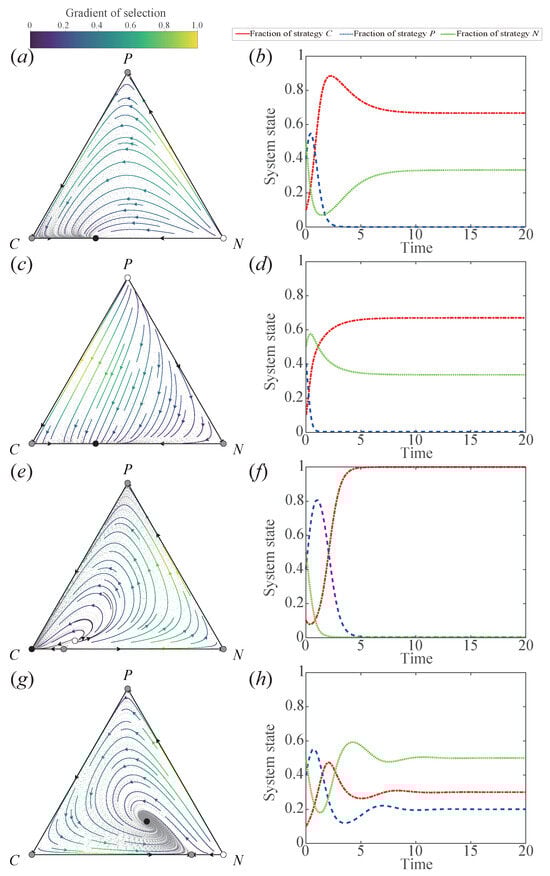Figure 4. In Panels (a,b), $Q=5, P=8, M=17$ and $N=14$, in Panels (c,d), $Q=5, P=8, M=17$ and $N=8$, in Panels (e,f), $Q=10, P=4, M=15$ and $N=13$, and in Panels (g,h), $Q=4, P=10, M=15$ and $N=13$. Other parameter values include: $R=10, C_2=5, F_1=5,$ and $F_2=8$.

As shown in Figure 4, regardless of the specific scenario, farmers will coexist with a certain proportion of completely adopting and not adopting conservation tillage technology. The strategies of partially adopting conservation tillage technology will disappear.

Example 5.

(1) 

When $P<M-R<Q\wedge M>N>R\wedge P(M-N)+Q(N-R)<PQ$, the system has five equilibria: three vertex points (only $(1,0,0)$ stable), one boundary saddle on $CN$, and an unstable interior equilibrium. Despite multistability, convergence to complete conservation tillage adoption occurs (Figure 4c), as proven in Appendix B (Case 7).

(2) 

For $Q<M-R<P\wedge M>N>R\wedge P(M-N)+Q(N-R)<PQ$, the unstable boundary equilibrium and corner equilibrium points contrast with a stable interior equilibrium point. This regime achieves three-strategy coexistence through asymptotically stable mixing ratios (Figure 4d), as rigorously derived in Appendix B (Case 12).

4. Conclusions

This study has developed an evolutionary game model to investigate the dynamics of CTT adoption, integrating the critical factors of heterogeneous time preferences (discount rate r), the lemon market effect (benefit P and loss Q), and technological externalities. Our findings yield specific and actionable insights for policymakers.

An individual farmer’s degree of time preference constitutes a key intrinsic factor influencing their adoption decision regarding CTT. Specifically, farmers with a higher time preference tend to heavily discount the long-term ecological benefits and economic returns. This cognitive bias, seriously hinders the promotion of CTT. The relationship between lemon market parameters P and Q dictates the system’s evolutionary stable state: When $P>Q$, the three strategies—complete adoption, partial adoption, and non-adoption—can coexist in stable proportions, offering a viable though not ideal outcome. When $P<Q$, the system exhibits unpredictable heteroclinic cycles, posing a significant barrier to stable adoption. When $P=Q$, the system forms a conservative Hamiltonian system with stable periodic oscillations, preventing convergence to any equilibrium and demonstrating the insufficiency of market forces alone to drive optimal outcomes. Based on these dynamics, we propose the following targeted policy interventions:

(1)

When $P>Q$ (Stable Coexistence): Policy should focus on strengthening market mechanisms, such as supporting third-party eco-label certifications to enhance the premium (P) for green products.

(2)

When $P<Q$ (Unpredictable Cycles): Intervention is critical. Establishing government-backed information disclosure platforms and introducing targeted subsidies to offset the loss Q can level the playing field for adopters.

(3)

When $P=Q$ (Periodic Oscillations): Continuous oversight is needed to disrupt the equilibrium, for instance, by increasing Pthrough public procurement policies for sustainable products or decreasing Q via stricter enforcement against false marketing.

To achieve the ideal state of universal CTT adoption, specific conditions must be met, offering clear policy targets: Condition 1: When $M>N>R$ and $P(M-N)+Q(N-R)\ne PQ$, the system can achieve the ideal state. This means the government must ensure that the benchmark return for complete adoption is the highest, partial adoption is intermediate, and non-adoption is the lowest, thereby providing farmers with a step-by-step ladder for technological improvement. Simultaneously, satisfying $P(M-N)+Q(N-R)\ne PQ$ ensures the system avoids entering periodic oscillations, preventing farmers from repeatedly switching between different strategies. Condition 2: When $M-R>Q, M-R>P$, and $M>N$, the system can achieve the ideal state. This sets clear target thresholds for policy intervention: it requires that the net technology return ($M-R$) must cover the lemon market loss Q caused by information asymmetry, that the net technology return from complete adoption ($M-R$) outstrips the fraudulent lemon market benefit P obtained by non-adopters, ensuring the non-adoption strategy cannot gain an advantage through fraudulent returns. Concurrently, the benchmark return for complete adoption M must be higher than that for partial adoption N, preventing farmers from stagnating at partial adoption. To address high time preferences, governments should design financial instruments, such as subsidized credit with grace periods aligned with CTT’s return cycle (e.g., 1–2 years), to alleviate short-term cost pressures. Furthermore, output-based contracts that guarantee premium prices can make long-term benefits more immediately tangible, effectively lowering the perceived discount rate r.

In summary, this study provides a dynamic analytical framework for CTT adoption, overcoming the limitations of static models. The integrated analysis of time preference and market failure offers a theoretical basis for designing sustainable agricultural policies in developing countries. However, it should be noted that this study has limitations, as we considered only three discrete adoption strategies. Future research could incorporate a continuous strategy space reflecting varying levels of CTT adoption. Moreover, while current homogeneous group models are useful for focusing on core mechanisms, they inevitably oversimplify real-world complexity. Future research could enhance the models’ practical explanatory capacity by incorporating factors such as social networks, spatial heterogeneity effects, and diffusion patterns. Analyzing its impact on system stability and convergence paths would advance our understanding of the complex systems driving agricultural green transition and ultimately provide more actionable scientific guidance for policymaking.

References

- Zhang, Y.Z.; Hu, Y.F.; Han, Y.Q.; Zhan, S. Spatial distribution and evolution of global major ecological degradation zones and research hotspots. Acta Ecol. Sin. 2021, 41, 7599–7613. [Google Scholar]
- Wu, Y.X.; Ren, X.H.; Yan, J.W.; Sun, Z.Y.; Jian, J.S. Bibliometric analysis of soil erosion research in runoff plots based on web of science from 1992 to 2023. J. Water Resour. Water Eng. 2024, 35, 212–224. [Google Scholar]
- Uri, N. The effect of energy on the adoption of conservation tillage in the united states. Environ. Geol. 1999, 37, 9–18. [Google Scholar] [CrossRef]
- Wollni, M.; Lee, D.R.; Thies, J.E. Conservation agriculture, organic marketing, and collective action in the honduran hillsides. Agric. Econ. 2010, 41, 373–384. [Google Scholar] [CrossRef]
- Nazu, S.B.; Saha, S.M.; Hossain, M.E.; Haque, S.; Khan, M.A. Willingness to pay for adopting conservation tillage technologies in wheat cultivation: Policy options for small-scale farmers. Environ. Sci. Pollut. Res. 2022, 29, 63458–63471. [Google Scholar] [CrossRef] [PubMed]
- Miao, S.; Chen, B.; Jiang, N. Collaboration among governments, agribusinesses, and rural households for improving the effectiveness of conservation tillage technology adoption. Sci. Rep. 2025, 15, 45. [Google Scholar] [CrossRef] [PubMed]
- Vitale, J.D.; Godsey, C.; Edwards, J.; Taylor, R. The adoption of conservation tillage practices in oklahoma: Findings from a producer survey. J. Soil Water Conserv. 2011, 66, 250–264. [Google Scholar] [CrossRef]
- Guo, H.; Zhao, W.; Pan, C.; Qiu, G.; Xu, S.; Liu, S. Study on the influencing factors of farmers’ adoption of conservation tillage technology in black soil region in china: A logistic-ism model approach. Int. J. Environ. Res. Public Health 2022, 19, 7762. [Google Scholar] [CrossRef]
- Qu, Y.; Pan, C.; Guo, H. Factors affecting the promotion of conservation tillage in black soil—The case of northeast china. Sustainability 2021, 13, 9563. [Google Scholar] [CrossRef]
- McCord, P.F.; Cox, M.; Schmitt-Harsh, M.; Evans, T. Crop diversification as a smallholder livelihood strategy within semi-arid agricultural systems near mount kenya. Land Use Policy 2015, 42, 738–750. [Google Scholar] [CrossRef]
- Grabowski, P.P.; Kerr, J.M. Resource constraints and partial adoption of conservation agriculture by hand-hoe farmers in mozambique. Int. J. Agric. Sustain. 2014, 12, 37–53. [Google Scholar] [CrossRef]
- Wang, Z.; Liu, Q.; Jiang, J. Can technology demonstration promote rural households’ adoption of conservation tillage in china? Econ. Res.-Ekon. Istraž. 2023, 36, 1–20. [Google Scholar] [CrossRef]
- Mu, L.; Luo, C.; Li, Y.; Tan, Z.; Gao, S. ‘They adopt, I also adopt’: The neighborhood effects and irrigator farmers’ conversion to adopt water-saving irrigation technology. Agric. Water Manag. 2024, 305, 109141. [Google Scholar] [CrossRef]
- Gathala, M.K.; Timsina, J.; Islam, M.S.; Rahman, M.M.; Hossain, M.I.; Harun-Ar-Rashid, M.; Ghosh, A.K.; Krupnik, T.J.; Tiwari, T.P.; McDonald, A. Conservation agriculture based tillage and crop establishment options can maintain farmers’ yields and increase profits in south asia’s rice–maize systems: Evidence from bangladesh. Field Crops Res. 2015, 172, 85–98. [Google Scholar] [CrossRef]
- Qin, W.; Niu, L.; You, Y.; Cui, S.; Chen, C.; Li, Z. Effects of conservation tillage and straw mulching on crop yield, water use efficiency, carbon sequestration and economic benefits in the loess plateau region of china: A meta-analysis. Soil Tillage Res. 2024, 238, 106025. [Google Scholar] [CrossRef]
- Wu, F.; Ma, J. Evolution dynamics of agricultural internet of things technology promotion and adoption in china. Discrete Dyn. Nat. Soc. 2020, 2020, 1854193. [Google Scholar] [CrossRef]
- Dong, J.; Chen, J.; Zhang, Y.; Cong, L.; Dean, D.; Wu, Q. Examining the value realization of ecological agricultural products in China: A tripartite evolutionary game analysis. J. Environ. Manag. 2025, 374, 124134. [Google Scholar] [CrossRef]
- Yu, Y.; He, Y.; Zhao, X. Impact of demand information sharing on organic farming adoption: An evolutionary game approach. Technol. Forecast. Soc. Change 2021, 172, 121001. [Google Scholar] [CrossRef]
- Nakagawa, Y.; Yokozawa, M. A social system to disperse the irrigation start date based on the spatial public goods game. PLoS ONE 2023, 18, e0286127. [Google Scholar] [CrossRef]
- Conley, T.G.; Udry, C.R. Learning about a new technology: Pineapple in ghana. Am. Econ. Rev. 2010, 100, 35–69. [Google Scholar] [CrossRef]
- Simutowe, E.; Ngoma, H.; Manyanga, M.; Silva, J.V.; Baudron, F.; Nyagumbo, I.; Kalala, K.; Habeenzu, M.; Thierfelder, C. Risk aversion, impatience, and adoption of conservation agriculture practices among smallholders in zambia. Heliyon 2024, 10, e12345. [Google Scholar] [CrossRef] [PubMed]
- Abedullah; Kouser, S. Evaluating the determinants of pesticide residues in vegetables: A case of lemon market in pakistan. J. Anim. Plant Sci. 2020, 30, 1525–1532. [Google Scholar] [CrossRef]
- FAO. Soil Tillage in Africa: Needs and Challenges; FAO Soils Bulletin; FAO: Rome, Italy, 1993; Volume 69. [Google Scholar]
- Shuval, K.; Stoklosa, M.; Pachucki, M.C.; Yaroch, A.L.; Drope, J.; Harding, M. Economic preferences and fast food consumption in us adults: Insights from behavioral economics. Prev. Med. 2016, 93, 204–210. [Google Scholar] [CrossRef] [PubMed]
- Laubach, T.; Williams, J.C. Measuring the natural rate of interest. Rev. Econ. Stat. 2003, 85, 1063–1070. [Google Scholar] [CrossRef]
- Wu, H.; Ge, Y.; Li, J. Uncertainty, time preference and households’ adoption of rooftop photovoltaic technology. Energy 2023, 276, 127456. [Google Scholar] [CrossRef]
- Pajewski, T.; Malak-Rawlikowska, A.; Gołębiewska, B. Measuring regional diversification of environmental externalities in agriculture and the effectiveness of their reduction by EU agri-environmental programs in poland. J. Clean. Prod. 2020, 276, 123013. [Google Scholar] [CrossRef]
- Mocan, N. Can consumers detect lemons? An empirical analysis of information asymmetry in the market for child care. J. Popul. Econ. 2007, 20, 743–780. [Google Scholar] [CrossRef]
- Taylor, P.D.; Jonker, L.B. Evolutionary stable strategies and game dynamics. Math. Biosci. 1978, 40, 145–156. [Google Scholar] [CrossRef]
- Huang, F.; Chen, X.; Wang, L. Evolution of cooperation in a hierarchical society with corruption control. J. Theor. Biol. 2018, 449, 60–72. [Google Scholar] [CrossRef]
- Liu, L.; Chen, X. Evolution of public cooperation in a risky society with heterogeneous assets. Front. Phys. 2018, 5, 67. [Google Scholar] [CrossRef]
- Wang, M.; Li, Y.; Cheng, Z.; Zhong, C.; Ma, W. Evolution and equilibrium of a green technological innovation system: Simulation of a tripartite game model. J. Clean. Prod. 2021, 278, 123944. [Google Scholar] [CrossRef]
- Shi, T.; Han, F.; Chen, L.; Shi, J.; Xiao, H. Study on value co-creation and evolution game of low-carbon technological innovation ecosystem. J. Clean. Prod. 2023, 414, 137720. [Google Scholar] [CrossRef]
- Guo, R.; Liu, L.; Liu, Y.; Zhang, L. Evolution of trust in a hierarchical population with different investors based on investment behavioral theory. Chaos Solitons Fractals 2023, 176, 114078. [Google Scholar] [CrossRef]
- Szolnoki, A.; Perc, M. Reward and cooperation in the spatial public goods game. Europhys. Lett. 2010, 92, 38003. [Google Scholar] [CrossRef]
- Szolnoki, A.; Mobilia, M.; Jiang, L.L.; Szczesny, B.; Rucklidge, A.M.; Perc, M. Cyclic dominance in evolutionary games: A review. J. R. Soc. Interface 2014, 11, 20140735. [Google Scholar] [CrossRef] [PubMed]
- Ma, Z.; Zhou, Y. Characterization and Stability Methods for Ordinary Differential Equations; Science Press: Beijing, China, 2001. [Google Scholar]
- Fernández Domingos, E.; Santos, F.C.; Lenaerts, T. Egttools: Evolutionary game dynamics in python. iScience 2023, 26, 106419. [Google Scholar] [CrossRef] [PubMed]
- Nowak, M. Evolutionary Dynamics: Exploring the Equations of Life; Harvard University Press: Cambridge, MA, USA, 2007; pp. 57–60. [Google Scholar]
Disclaimer/Publisher’s Note: The statements, opinions and data contained in all publications are solely those of the individual author(s) and contributor(s) and not of MDPI and/or the editor(s). MDPI and/or the editor(s) disclaim responsibility for any injury to people or property resulting from any ideas, methods, instructions or products referred to in the content. |
© 2025 by the authors. Licensee MDPI, Basel, Switzerland. This article is an open access article distributed under the terms and conditions of the Creative Commons Attribution (CC BY) license (https://creativecommons.org/licenses/by/4.0/).