Reversible Conversion Formulas Based on Partial Symmetric Linear Regression Models

Abstract

Symmetric regression deals with a reversible functional relationship involving a set of variables, where all of them are measured with error and it is not meaningful to consider one as the response and the remaining ones as explanatory. Therefore, it is unsuitable to study any functional (linear) relationship between them by fixing one direction of the regression rather than the other. The scope of the symmetric regression can be expanded by considering a partial symmetric linear regression where the functional relationship is controlled for other variables, which are not assumed to be error-prone. Actually, the word partial in this context, means that we are not interested in a fully symmetric relationship between all the variables but in a symmetric and reversible relationship that holds for some variables of interest, whose functional relationship is of primary concern, for any given value of the control variables. Therefore, a partial symmetric regression modeling strategy is developed within a very general framework that includes different symmetric regression strategies. The finite sample behaviors of the proposed estimators are investigated through numerical studies and illustrated with an application to rheumatology data to find a reversible conversion formula between the Stanford Health Assessment Questionnaire (HAQ) score and the Multi-Dimensional HAQ (MDHAQ) score.

1. Introduction

Symmetric regression concerns the study of a functional relationship among a set of variables through a regression model specification without distinguishing between the response and the explanatory variables [1,2,3]. In other words, symmetric regression deals with a reversible functional relationship, regardless of the direction of regression, involving variables that are all supposed to be measured with error [4]. For simplicity and without loss of generality, let us start off with the bivariate case. For example, the variables $(Y,X)$ may refer to measurements of the same quantity using two (or more) different devices or assays, or may be intrinsically related measures from a clinical or physical point of view, for which we cannot make a clear distinction between response and predictors. In this situation, inference using the symmetric regression model allows us to assess the statistical equivalence or evaluate the bias of measurements conducted by using different tools or methodologies, and to assess their statistical equivalence and practical interchangeability in providing the same results notwithstanding the measurement errors. The study of reversible functional relationships is of interest in many fields, such as physics, economics, social sciences, psychology, biostatistics, astronomy, chemistry, geodesy, allometry, and in general for all those situations where it is meaningful to consider regression in any direction.

In classical simple linear regression, it is possible to consider two different models depending on which variable is assumed to be the response. Let $E\left(Y\right|X=x)={\mu }_Y\left(x\right)$ be the conditional expectation of Y for a given x and $E\left(X\right|Y=y)={\mu }_X\left(y\right)$ be the conditional expectation of X for a given y. The simple linear regression of Y on X corresponds to ${\mu }_Y\left(x\right)=\alpha +\beta x$, and the simple linear regression of X on Y is given by ${\mu }_X\left(y\right)=\gamma +\delta y$. The requirement of symmetry is that the two regression equations are reversible, that is, they are the inverse of each other, with $\gamma =-\alpha /\beta$ and $\delta =1/\beta$. Unfortunately, although not fully recognized, the ordinary least squares (OLS) fit is not symmetric since predictions depend on which variable is selected as the response and which variable is selected as the (fixed) explanatory variable; that is, ${\mu }_Y\left({\mu }_X\left(y\right)\right)\ne {\mu }_X^{-1}\left({\mu }_Y\left(x\right)\right)$, where ${\mu }_X^{-1}\left(y\right)$ denotes the regression of X on Y expressed in y-units unless a perfect correlation exists among the variables. In contrast, within a symmetric linear regression framework, one is interested in establishing a reversible conversion formula between the pair of measurements; that is, it is expected to predict X from Y and Y from X in a reversible fashion, meaning that the two predictions can be obtained one from another, removing the lack of reversibility of OLS regression and providing us with a reversible conversion formula between the predicted values of Y and X. In other words, we are interested in estimating a true functional relationship between variables rather than predicting one variable based on known values of the other variable. Moreover, in the presence of measurement errors, OLS gives rise to biased estimates of the regression coefficients and leads to inconsistent conclusions when the roles of the variables are interchanged, a phenomenon called the regression paradox [5].

Several modifications of OLS are available that extend it to the case of simultaneous regression in all directions. The first version of symmetric regression is orthogonal regression (OR), as introduced in [6] and also based on the work in [7,8]. A second version is geometric mean regression (GMR) [9,10,11], also known as reduced major axis, diagonal, or impartial regression. The main improvement over OR is that GMR is scale independent. Additional versions include Pythagorean regression (PR) [12] and Deming regression (DR) [13,14,15]. While OR, GMR, and PR are meant to deal with equal measurement errors’ variances and the homoschedastic setting, DR is a general approach to symmetric regression that allows us to take into account different measurement errors in the variables Y and X and across observations. All the symmetric regression methods discussed above can be extended to the multiple linear regression setting, where the goal is to model a functional linear relationship between Y and a set of variables $\mathbf{X}=(X_1,X_2,\dots ,X_p)$, with $p>1$.

In this work, we focus on modeling the symmetric linear regression relationship between Y and $\mathbf{X}$ while adjusting for the effect of additional control covariates, denoted by $\mathbf{Z}=(Z_1,Z_2,\dots ,Z_q)$, with $q\ge 1$. Specifically, we do not aim to identify a fully reversible dependence structure among all the variables $(Y,\mathbf{X},\mathbf{Z})$ but rather a symmetric relationship between Y and $\mathbf{X}$ that is conditional on given values $\mathbf{z}$ of $\mathbf{Z}$ such that

$${\mu }_Y({\mu }_{\mathbf{X}}\left(y\right),\mathbf{z})={\mu }_{\mathbf{X}}^{-1}({\mu }_Y\left(\mathbf{x}\right),\mathbf{z}),\forall \mathbf{z}$$

where, with a slight abuse of notation, ${\mu }_{\mathbf{X}}^{-1}(y,\mathbf{z})$ denotes the prediction from the regression of $\mathbf{X}$ on $(Y,\mathbf{Z})$ expressed in y-units, $\mathbf{x}=(x_1,x_2,\dots ,x_p)$, and $\mathbf{z}=(z_1,z_2,\dots ,z_q)$. The proposed methodology is very general and designed to be applicable to every symmetric regression version listed above.

The remainder of the paper is structured as follows: some necessary background on symmetric regression is provided in Section 2; the partial symmetric linear regression approach is introduced in Section 3, and the model fitting is developed as well; numerical studies and an empirical application from rheumatology are covered in Section 4; finally, a discussion concludes the paper in Section 5.

2. Background

Assume that the interest lies in comparing pairs of measurements $(y_i,x_i)$ taken on n units by two alternative methods, $i=1,2,\dots ,n$. The symmetric linear regression model for $(Y,X)$ states that

$$\left\{\begin{array}{c}{x}_i=u_i+{\eta }_i\hfill \\ y_i=v_i+{ϵ}_i\hfill \end{array}\right.$$

(1)

with $v_i=\alpha +\beta u_i$; that is, the true (but unobservable) values $(u_i,v_i)$ are linked by a linear regression with slope $\beta$ and intercept $\alpha$. The error terms ${\eta }_i$ and ${ϵ}_i$ are realizations of independent random variables with null expectations and constant equal variances; that is, $Var\left({\eta }_i\right)=Var\left({ϵ}_i\right)={\sigma }^2$. The model in (1) is also referred to as the Errors-In-Variables model [16,17]. Under the assumptions of model (1), we have

$$\left\{\begin{array}{c}{\mu }_Y\left(x\right)=\alpha +\beta x={\mu }_Y+\beta (x-{\mu }_X)\hfill \\ {\mu }_X\left(y\right)={\displaystyle \frac{1}{\beta }}(y-\alpha )={\mu }_X+{\displaystyle \frac{1}{\beta }}(y-{\mu }_Y)\hfill \end{array}\right.$$

(2)

where ${\mu }_Y\left(x\right)$ and ${\mu }_X\left(y\right)$ are the conditional expectations of Y and X, respectively. The model specification clearly requires that $\beta \ne 0$. Here, ${({\mu }_Y,{\mu }_X)}^{\top }$ denotes the vector of marginal expectations. We note that the same set of regression coefficients determines the regression lines in both directions.

To estimate the parameter $(\alpha ,\beta )$ of the symmetric regression, one should take into account both y- and x-errors. Obviously, it is not sufficient to minimize the sum of squared errors only in one direction, as for OLS. Rather, it is necessary to define a suitable objective function to be minimized that is based on a summary of both squared vertical $d_y^2={(y-{\mu }_Y\left(x\right))}^2$ and horizontal $d_x^2={(x-{\mu }_X\left(y\right))}^2$ distances. From (2), we note that $d_y^2={\beta }^{-2}{d}_x^2$. In the following, we review some of the most popular versions of symmetric regression as listed in Section 1 (see [3] for a review).

The OLS fit of the regression of Y on X minimizes the sum of squared vertical errors (the segment BP in Figure 1) $Q_{Y|X}\left(\beta \right)={\sum }_{i=1}^n{d}_{y_i}^2$; the OLS fit of the regression of X on Y minimizes the sum of squared horizontal errors (the segment AP in Figure 1) $Q_{X|Y}\left(\beta \right)={\sum }_{i=1}^n{d}_{x_i}^2$. The GMR is defined considering the minimization of the sum of the geometric mean of the squared vertical and horizontal distances; that is,

$$Q_{GMR}\left(\beta \right)=\sum _{i=1}^n\sqrt{d_{y_i}^2{d}_{x_i}^2}={\displaystyle \frac{1}{\left|\beta \right|}}\sum _{i=1}^n{d}_{y_i}^2,$$

for $\left|\beta \right|>0$. This is equivalent to the minimization of the sum of the areas of the ABP triangles in Figure 1 generated from the projections of the points on the line. We further note that GMR can also be obtained as the maximum agreement linear predictor maximizing the Lin’s concordance correlation coefficient [18] between Y and its predicted value ${\mu }_Y\left(x\right)$. The PR is obtained from the minimization of the sum of the arithmetic mean of the squared distances, so the criterion is

$$Q_{PR}\left(\beta \right)=\sum _{i=1}^n\left(d_{y_i}^2+d_{x_i}^2\right)=\left(1+{\displaystyle \frac{1}{{\beta }^2}}\right)\sum _{i=1}^n{d}_{y_i}^2,$$

for $\left|\beta \right|>0$. This is equivalent to finding the best line minimizing the sum of the squared hypotenuses AB in Figure 1 of the triangles formed by the data points and the line. The OR is obtained from the minimization of the sum of the harmonic mean of the squared vertical and horizontal distances, which leads to the same result as minimizing the sum of the squared orthogonal distances (PH in Figure 1). The squared orthogonal distance from the regression line can be expressed as

$$d_o^2={\displaystyle \frac{d_x^2{d}_y^2}{d_y^2+d_x^2}}={\displaystyle \frac{d_y^2}{1+{\beta }^2}};$$

and then the criterion becomes

$$Q_{OR}\left(\beta \right)={\displaystyle \frac{1}{1+{\beta }^2}}\sum _{i=1}^n{d}_{y_i}^2.$$

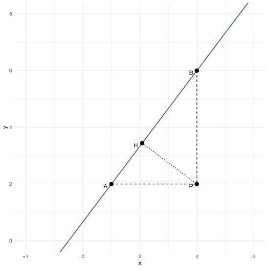
Figure 1. Geometry of symmetric regression.

It is worth noting that the OR solution also corresponds to maximum likelihood estimation of the Errors-In-Variables model (1).

The DR [14] provides a more general solution to the problem of maximum likelihood estimation of the EIV model in (1). Actually, under no restrictions on the error variances, the objective function for the (weighted) DR becomes

$$Q_{DR}\left(\beta \right)=\sum _{i=1}^n{w}_i\left(\beta \right)d_{y_i}^2\left(\beta \right)$$

with $w_i\left(\beta \right)={({\sigma }_{y_i}^2+{\beta }^2{\sigma }_{x_i}^2)}^{-1}$. The variances can be estimated from replicated measurements. Under the hypothesis of proportional variances ${\sigma }_x^2=k{\sigma }_y^2$, then

$$Q_{DR}\left(\beta \right)={\displaystyle \frac{1}{1+k{\beta }^2}}\sum _{i=1}^n{d}_{y_i}^2\left(\beta \right).$$

In practice, when k is not known in advance based on available knowledge, it is estimated using multiple measurements for each subject. We note that OR is recovered for $k=1$. The reader is referred to [3] for a discussion about the effect of the variance ratio k on the bias of the estimators for $(\alpha ,\beta )$ for the different methods described above. In summary, all the methods lead to (asymptotically) unbiased estimates when the error terms have the same variance, but OR, GMR, and PR exhibit some bias when the variance ratio moves away from unity. In contrast, DR is (asymptotically) unbiased regardless of the variance ratio. Additional details on the effect of the variance ratio on inference can be found in [19].

We note that, in all cases, the objective function can be written as $Q\left(\beta \right)=g\left(\beta \right){\sum }_{i=1}^n{d}_{y_i}^2\left(\beta \right)$, with $g(·)>0$, hence enabling unified treatment of all considered symmetric regressions. The estimating equation for the slope parameter $\beta$ takes the general form

$$\begin{array}{ccc}\hfill \Psi \left(\beta \right)& =& \sum _{i=1}^n\psi \left(\beta \right)=\sum _{i=1}^n\left[g^{\prime }\left(\beta \right)d_{y_i}^2\left(\beta \right)-2\beta d_{y_i}\left(\beta \right)x_i\right]\hfill \\ & =& g^{\prime }\left(\beta \right)[s_y^2-2\beta s_{yx}+{\beta }^2{s}_x^2]-2g\left(\beta \right)[s_{yx}-\beta s_x^2]=0\hfill \end{array}$$

(3)

where $g^{\prime }\left(\beta \right)$ denotes the first derivative of $g\left(\beta \right)$ and $s_y^2,s_x^2,$ and $s_{yx}$ are the sample variance of Y, the sample variance of X, and their covariance, respectively. The estimate for the intercept term is always given by $\widehat{\alpha }=\overline{y}-\widehat{\beta }\overline{x}$, where $\overline{y}$ and $\overline{x}$ are the sample means and $\widehat{\beta }$ is the fitted slope obtained from (3). All the symmetric regression lines pass through the point of coordinates $(\overline{y},\overline{x})$ as the OLS regression lines. For the cases of OR, GMR, and DR, the estimating equation for the slope is quadratic in $\beta$. The estimate of $\beta$ corresponds to the solution with the same sign as the correlation between $(Y,X)$. For GMR, the fitted slope is ${\hat{\beta }}_{GMR}=\mp {\displaystyle \frac{s_y^2}{s_x^2}}$. The solutions for DR are

$${\hat{\beta }}_{DR}={\displaystyle \frac{1}{2k{s}_{xy}}}\left[(k{s}_y^2-s_x^2)\mp \sqrt{{(k{s}_y^2-s_x^2)}^2+4k{s}_{xy}^2}\right].$$

The estimating equation for the slope of the PR is quartic [12]; the estimate ${\hat{\beta }}_{PR}$ is one of two real solutions sharing the same sign as $s_{yx}$.

Even though, for simplicity, we have focused on the special case of a pair of measurement methods for the same underlying quantity, the symmetric regression methods described above can be generalized to situations where the interest is in modeling a reversible linear relationship among a set of $(p+1)$, $p>1$ variables, which we prefer to denote as $(Y,\mathbf{X})$ [20]. Now, the $y$- and $x_j$-distances, $j=1,2,\dots ,p$, from the hyperplane ${\mu }_Y\left(\mathbf{x}\right)=\alpha +{\sum }_{j=1}^p{\beta }_j{x}_j$ are

$$d_y=\left[y-\left(\alpha +\sum _{j=1}^p{\beta }_j{x}_j\right)\right]$$

and $d_{x_j}={\left|{\beta }_j\right|}^{-1}{d}_y$. Then, GMR, PR, and OR correspond to the geometric, arithmetic, and harmonic means of $d_y^2,d_{x_1}^2,\dots ,d_{x_p}^2$, respectively. Let $\mathit{\beta }=({\beta }_1,{\beta }_2,\dots ,{\beta }_p)$. In the case of GMR,

$$g(\mathit{\beta })={\left(\prod _{j=1}^p{\beta }_j^{-2}\right)}^{{\displaystyle \frac{1}{p+1}}},$$

with $|{\beta }_j|>0,\forall j$; for PR, the arithmetic mean leads to

$$g(\mathit{\beta })=\left(1+\sum _{j=1}^p{\beta }_j^{-2}\right),$$

with $|{\beta }_j|>0,\forall j$; for OR, using the harmonic mean, we have

$$g(\mathit{\beta })={\left(1+\sum _{j=1}^p{\beta }_j^2\right)}^{-1}.$$

Standard errors can be obtained using first-order approximations based on the Delta method [21], the general theory of M-estimators [22], the influence function approach [23], the method of moments [24], the leave-one-out jackknife [15,25], and the pair (or nested) bootstrap [26,27].

3. Material and Methods

In this section, we first introduce the partial symmetric regression model, and then we focus on estimating the corresponding reversible conversion equations. In addition to the error-prone measurements $(Y,\mathbf{X})$, assume that we also collect data on some control variables $\mathbf{Z}=(Z_1,Z_2,\dots ,Z_q)$, $q\ge 1$. The control variables $\mathbf{Z}$ are not measured with error, and they describe features that may affect the functional relationship involving $(Y,\mathbf{X})$, such as sex, age, disease status, etc. For ease of illustration, let us consider the case of a simple partial linear functional relationship for given $\mathbf{z}=(z_1,z_2,\dots ,z_q)$, that is, when $(Y,X)$ is bivariate. Given the data $(y_i,x_i,{\mathbf{z}}_i)$, $i=1,2,\dots ,n$, the partial symmetric regression model states that

$$\left\{\begin{array}{c}{x}_i=u_i+{\eta }_i\hfill \\ y_i=v_i+{\gamma }^{\top }\mathbf{z}+{ϵ}_i\hfill \end{array}\right.$$

(4)

with $v_i=\alpha +\beta u_i$ and $\gamma =({\gamma }_1,{\gamma }_2,\dots ,{\gamma }_q)$. In terms of conditional expectations, under the assumptions already made for model (1), the reversible regression equations between Y and X, while controlling for $\mathbf{Z}$, can be written as

$$\left\{\begin{array}{c}{\mu }_Y(x,z)=\alpha +\beta x+{\gamma }^{\top }\mathbf{z}\hfill \\ {\mu }_X(y,z)={\displaystyle \frac{1}{\beta }}\left(y-\alpha -{\gamma }^{\top }\mathbf{z}\right)\hfill \end{array}\right.$$

(5)

for $\beta \ne 0$. Let us assume that $(Y,X,\mathbf{Z})$ has finite second-order moments with the mean vector and variance–covariance matrix given by $\mu ={({\mu }_Y,{\mu }_X,{\mu }_{\mathbf{Z}})}^{\top }$ and

$$\Sigma =\left(\begin{array}{ccc}{\Sigma }_{YY}& {\Sigma }_{YX}& {\Sigma }_{Y\mathbf{Z}}\\ {\Sigma }_{YX}^{\top }& {\Sigma }_{XX}& {\Sigma }_{X\mathbf{Z}}\\ {\Sigma }_{Y\mathbf{Z}}^{\top }& {\Sigma }_{X\mathbf{Z}}^{\top }& {\Sigma }_{\mathbf{Z}\mathbf{Z}}\end{array}\right).$$

Actually, according to (5) and provided that ${\Sigma }_{\mathbf{Z}\mathbf{Z}}$ is positive definite (in order to be invertible), the best linear predictor of $(Y,X)$ given $\mathbf{Z}$ is the conditional expectation

$${\mu }_{(Y,X)}\left(\mathbf{z}\right)={\mu }_{(Y,X)}+\xi {\Sigma }_{\mathbf{Z}\mathbf{Z}}^{-1}\left(\mathbf{z}-{\mu }_{\mathbf{Z}}\right)$$

where ${\mu }_{(Y,X)}={({\mu }_Y,{\mu }_X)}^{\top }$ and $\xi =({\Sigma }_{Y\mathbf{Z}},{\Sigma }_{X\mathbf{Z}})$, implying that the model in (5) can be written as

$$\left\{\begin{array}{c}{\mu }_Y(x,z)={\mu }_Y+{\gamma }_{Y|\mathbf{Z}}(\mathbf{z}-{\mu }_{\mathbf{Z}})\hfill \\ {\mu }_X(y,z)={\mu }_X+{\gamma }_{X|\mathbf{Z}}(\mathbf{z}-{\mu }_{\mathbf{Z}})\hfill \end{array}\right.$$

(6)

where ${\gamma }_{Y|\mathbf{Z}}={\Sigma }_{Y\mathbf{Z}}{\Sigma }_{\mathbf{Z}\mathbf{Z}}^{-1}$ and ${\gamma }_{X|\mathbf{Z}}={\Sigma }_{X\mathbf{Z}}{\Sigma }_{\mathbf{Z}\mathbf{Z}}^{-1}$ are the slope coefficients of the regressions of Y on $\mathbf{Z}$ and X on $\mathbf{Z}$, respectively. Then, the model in (6) provides a direct and useful interpretation of the $\gamma$ coefficient vector: after replacing $u=(x-{\gamma }_{X|\mathbf{Z}}\mathbf{z}-\eta )$ and some simple algebra, one finds that

$$\gamma =({\gamma }_{Y|\mathbf{Z}}-\beta {\gamma }_{X|\mathbf{Z}}).$$

(7)

These findings apply straightforwardly to the case when the dimension of $\mathbf{X}$ is larger than one.

3.1. Model Fitting

Let us consider the model in (4), extended to the case of a reversible conversion formula between more than two variables, that is, between the $(p+1)$ variables $(Y,\mathbf{X})$. To fit a partial symmetric linear regression model for $(Y,\mathbf{X})$, one can build upon the background methodology described in Section 2. Let $\mathit{\theta }=(\alpha ,\mathit{\beta },\gamma )$, with $\mathit{\beta }=({\beta }_{!},{\beta }_2,\dots ,{\beta }_p)$. Here, it is proposed to minimize a combined measure of both squared y- and $x_j$-distances from the regression hyperplane, but not of squared $\mathbf{z}$-distances, assuming that ${\beta }_j\ne 0$, $j=1,2,\dots ,p$. The squared y- and $x_j$-distances from the regression hyperplane are

$$\begin{array}{ccc}\hfill d_y^2(\mathit{\theta })& =& {\left[y-(\alpha +{\mathit{\beta }}^{\top }\mathbf{x}+{\gamma }^{\top }\mathbf{z})\right]}^2\hfill \\ \hfill d_{x_j}^2(\mathit{\theta })& =& {\left[x_j-{\displaystyle \frac{1}{{\beta }_j}}\left(y-\alpha -{\mathit{\beta }}_{-j}^{\top }{\mathbf{x}}_{-j}-{\gamma }^{\top }\mathbf{z}\right)\right]}^2={\displaystyle \frac{1}{{\beta }_j^2}}{d}_y^2\left(\theta \right)\hfill \end{array}$$

where ${\mathit{\beta }}_{-j}$ is the coefficient vector without the j-th element, and ${\mathbf{x}}_{-j}$ corresponds to removing the j-th variable. After combining these distances using a suitable summary measure, we obtain an objective function of the general form

$$\begin{array}{ccc}\hfill Q(\mathit{\theta })& =& g(\mathit{\beta })\sum _{i=1}^n{d}_{y_i}^2(\mathit{\theta })=g(\mathit{\beta })\sum _{i=1}^n{\left[y_i-\left(\alpha +{\mathit{\beta }}^{\top }{\mathbf{x}}_i+{\gamma }^{\top }{\mathbf{z}}_i\right)\right]}^2\hfill \\ \hfill & =& g(\mathit{\beta })\sum _{i=1}^n{\left[y_i-\left(\overline{y}+{\mathit{\beta }}^{\top }({\mathbf{x}}_i-\overline{\mathbf{x}})+{\gamma }^{\top }({\mathbf{z}}_i-\overline{\mathbf{z}})\right)\right]}^2\hfill \end{array}$$

(8)

where the positive real-valued function $g(\mathit{\beta })$ depends on the selected version of symmetric regression, and $\alpha =\overline{y}-{\hat{\mathit{\beta }}}^{\top }\overline{\mathit{x}}-{\hat{\gamma }}^{\top }\overline{\mathbf{z}}$ with ${(\overline{y},\overline{\mathit{x}},\overline{\mathbf{z}})}^{\top }$ is the vector of sample means. The minimization of $Q(\mathit{\theta })$ through the use of partial derivatives leads to the set of estimating functions

$$\begin{array}{ccc}\hfill {\Psi }_{\alpha }(\mathit{\theta })={\displaystyle \frac{\partial Q(\mathit{\theta })}{\partial \alpha }}& =& -2g(\mathit{\beta })\sum _{i=1}^n{d}_{y_i}(\mathit{\theta })\hfill \end{array}$$

(9)

$$\begin{array}{ccc}\hfill {\Psi }_{{\mathit{\beta }}_j}(\mathit{\theta })={\displaystyle \frac{\partial Q(\mathit{\theta })}{\partial {\mathit{\beta }}_j}}& =& g_j^{\prime }(\mathit{\beta })\sum _{i=1}^n{d}_{y_i}^2(\mathit{\theta })-2g(\mathit{\beta })\sum _{i=1}^n{d}_{y_i}(\mathit{\theta })x_{ij}\hfill \end{array}$$

(10)

$$\begin{array}{ccc}\hfill {\Psi }_{\gamma }(\mathit{\theta })={\displaystyle \frac{\partial Q(\mathit{\theta })}{\partial \gamma }}& =& -2g(\mathit{\beta })\sum _{i=1}^n{d}_{y_i}(\mathit{\theta }){\mathbf{z}}_i,\hfill \end{array}$$

(11)

where $g_j^{\prime }(\mathit{\beta })$ is the derivative of $g(\mathit{\beta })$ with respect to ${\mathit{\beta }}_j$. We note that the estimating function ${\Psi }_{\gamma }(\mathit{\theta })$ in (11) corresponding to the control regression coefficient vector $\gamma$ resembles the classical one from OLS regression. In particular, the estimate of $\gamma$ for a given $\mathit{\beta }$ is obtained from the OLS regression of $Y-{\mathit{\beta }}^{\top }\mathit{X}$ on $\mathit{Z}$; the constrained estimate of $\gamma$ for a fixed $\mathit{\beta }$ is

$${\hat{\gamma }}_{\mathit{\beta }}={\left({\mathit{Z}}^{\top }\mathit{Z}\right)}^{-1}{\mathit{Z}}^{\top }y-\mathit{\beta }{\left({\mathit{Z}}^{\top }\mathit{Z}\right)}^{-1}{\mathit{Z}}^{\top }\mathit{x}={\hat{\gamma }}_{Y|\mathit{Z}}-{\mathit{\beta }}^{\top }{\hat{\gamma }}_{\mathit{X}|\mathit{Z}},$$

(12)

consistent with (7). The constrained estimate in (12) depends on the fitted coefficients of the OLS regression of Y on Z and X on Z, respectively. By substituting ${\hat{\gamma }}_{\mathit{\beta }}$ in (10), and also considering that ${\hat{\alpha }}_{\mathit{\beta }}=\overline{y}-{\mathit{\beta }}^{\top }\overline{\mathit{x}}-{\hat{\gamma }}_{\mathit{\beta }}^{\top }\overline{\mathbf{z}}$ from (9), we obtain a profile estimating function for $\mathit{\beta }$ whose components are ${\tilde{\Psi }}_{{\mathit{\beta }}_j}(\mathit{\beta })={\Psi }_{{\mathit{\beta }}_j}(\mathit{\beta },{\hat{\alpha }}_{\mathit{\beta }},{\hat{\gamma }}_{\mathit{\beta }})$.

In the special case of a bivariate $(Y,X)$, for GMR, OR, and DR, the profile estimating equation is again quadratic in $\beta$, whereas, for PR, it is still quartic. Let $s_y^2,s_x^2$ denote the sample variances of Y and X and $s_{yx}$ denote the sample covariance; $S_{\mathbf{z}\mathbf{z}}$ is the variance–covariance matrix for $\mathit{Z}$; $S_{y\mathbf{z}}$ and $S_{x\mathbf{z}}$ are the sample covariance matrices between $Y,\mathit{Z}$ and $X,\mathit{Z}$, respectively. We find that

$$\sum _{i=1}^n{d}_{y_i}^2(\beta ,\gamma )=n[s_y^2+s_x^2{\beta }^2+{\gamma }^{\top }{S}_{zz}\gamma -2s_{yx}\beta -2{\gamma }^{\top }{S}_{y\mathit{z}}+2\beta {\gamma }^{\top }{S}_{x\mathit{z}}]$$

and

$$\sum _{i=1}^n{d}_{y_i}(\beta ,\gamma )(x_i-\overline{x})=n[s_{yx}-s_x^2{\beta }^2-{\gamma }^{\top }{S}_{x\mathit{z}}]$$

Then, in the case of GMR, the profile estimating function is

$${\tilde{\Psi }}_{\beta }^{GMR}\left(\beta \right)=(s_x^2-{\hat{\gamma }}_{X|\mathit{Z}}^{\top }{S}_{x\mathit{z}}){\beta }^2-s_y^2,$$

whereas, for DR, we find that

$${\tilde{\Psi }}_{\beta }^{DR}\left(\beta \right)=A{\beta }^2-B\beta +C$$

with

$$\begin{array}{ccc}\hfill A& =& k{s}_{yx}(1-{\hat{\gamma }}_{Y|\mathit{Z}})\hfill \\ \hfill B& =& k(s_y^2-{\hat{\gamma }}_{Y|\mathit{Z}}^{\top }{S}_{y\mathit{z}})-(s_x^2-{\hat{\gamma }}_{X|\mathit{Z}}^{\top }{S}_{x\mathit{z}})\hfill \\ \hfill C& =& {\hat{\gamma }}_{X|\mathit{Z}}^{\top }{S}_{y\mathit{z}}-s_{yx}.\hfill \end{array}$$

The case $k=1$ coresponds to OR.

3.2. Interaction Terms

The model in (5) can be extended further to include interactions terms. Let us restrict our attention to the case with three univariate variables $(Y,X,Z)$. Now, we consider the functional linear relationship

$$\left\{\begin{array}{c}{\mu }_Y(x,z)=\alpha +{\beta }_{1}x+\gamma z+{\beta }_{2}xz\hfill \\ {\mu }_X(y,z)={\displaystyle \frac{1}{{\beta }_1+{\beta }_{2}z}}\left(y-\alpha -\gamma z\right)\hfill \end{array}\right.$$

(13)

where the interaction term between X and Z is now included, and $({\beta }_1+{\beta }_{2}z)\ne 0$ to guarantee existence. In this setting, the objective function to be minimized becomes

$$Q(\mathit{\theta })=\sum _{i=1}^{n}g({\beta }_1,{\beta }_2;z_i)d_{y_i}^2(\mathit{\theta }).$$

In the special case of partial GMR, we have that

$$g({\beta }_1,{\beta }_2;z_i)={|{\beta }_1+{\beta }_2{z}_i|}^{-1};$$

for PR

$$g({\beta }_1,{\beta }_2;z_i)={({\beta }_1+{\beta }_2{z}_i)}^{-2}+1;$$

and for OR

$$g({\beta }_1,{\beta }_2;z_i)={[{({\beta }_1+{\beta }_2{z}_i)}^2+1]}^{-1}.$$

The estimating functions for ${\beta }_1$ and ${\beta }_2$ change according to the different form of the function $g(·)$ and its partial derivatives. In particular, we have

$$\begin{array}{ccc}\hfill {\Psi }_{{\beta }_1}(\mathit{\theta })& =& \sum _{i=1}^n{g}_1^{\prime }({\beta }_1,{\beta }_2;z_i)d_{y_i}^2(\mathit{\theta })-2\sum _{i=1}^{n}g({\beta }_1,{\beta }_2;z_i)d_{y_i}(\mathit{\theta })x_i\hfill \\ \hfill {\Psi }_{{\beta }_2}(\mathit{\theta })& =& \sum _{i=1}^n{g}_1^{\prime }({\beta }_1,{\beta }_2;z_i)z_i{d}_{y_i}^2(\mathit{\theta })-2\sum _{i=1}^{n}g({\beta }_1,{\beta }_2;z_i)d_{y_i}(\mathit{\theta })x_i{z}_i\hfill \end{array}$$

where $g_1^{\prime }(·)$ denotes the first derivative with respect to ${\beta }_1$, and the first derivative with respect to ${\beta }_2$ is $z_i{g}_1^{\prime }(·)$.

In particular, when the control variable Z is categorical with ℓ levels, fitting the model specified in (13) corresponds to fitting a separate symmetric regression model within each level of Z, thereby allowing the relationship between Y and X to vary across the strata defined by the levels of the control variable not only with regard to the intercept but also with regard to the slope. In this situation, ${\mathbf{z}}_i=(z_{i2},z_{i3},\dots ,z_{i\ell })$ is the vector of observations from the set of binary variables corresponding to the levels of Z and ${\mathit{\beta }}_{\mathbf{2}}=({\beta }_{22},{\beta }_{23},\dots ,{\beta }_{2\ell })$.

3.3. Uncertainty Evaluation

The proposed estimator $\hat{\mathit{\theta }}=(\hat{\alpha },\hat{\mathit{\beta }},\hat{\gamma })$ belongs to the general class of M-estimators since the estimating function $\Psi =\Psi (\mathit{\theta })$ defined through (9)–(11) can be written as the sum of n individual contributions; that is, $\Psi ={\sum }_{i=1}^n{\psi }_i$, with ${\psi }_i={\psi }_i(\mathit{\theta })$ denoting the individual contribution to the estimating function from the $i^{th}$ observation. Then, the asymptotic distribution of $\hat{\mathit{\theta }}$ is

$$\sqrt{n}(\hat{\mathit{\theta }}-\mathit{\theta })\sim N(0,V(\mathit{\theta }))$$

with $V=V(\mathit{\theta })={\sigma }^2{M}^{-1}\Omega M^{-1}$, where $\sigma$ is the regression measure of scale, $M=E[-{\psi }^{\prime }(\mathit{\theta })]$, and $\Omega =E\left[\psi (\mathit{\theta })\psi {(\mathit{\theta })}^{\top }\right]$. Here, ${\psi }^{\prime }(\mathit{\theta })$ is the matrix of second partial derivatives with elements

$${\psi }^{\prime }(\mathit{\theta })=\left(\begin{array}{ccc}{\psi }_{\alpha \alpha }& {\psi }_{\alpha \mathit{\beta }}& {\psi }_{\alpha \gamma }\\ {\psi }_{\alpha \mathit{\beta }}^{\top }& {\psi }_{\mathit{\beta }\mathit{\beta }}& {\psi }_{\mathit{\beta }\gamma }\\ {\psi }_{\alpha \gamma }^{\top }& {\psi }_{\mathit{\beta }\gamma }^{\top }& {\psi }_{\gamma \gamma }\end{array}\right).$$

An estimate of the asymptotic variance of $\hat{\mathit{\theta }}$ can be obtained using the empirical counterparts of M and $\Omega$

$$\begin{array}{ccc}\hfill \hat{M}& =& n^{-1}\sum _{i=1}^n{\psi }_i^{\prime }(\mathit{\theta })\hfill \\ \hfill \hat{\Omega }& =& n^{-1}\sum _{i=1}^n{\psi }_i(\mathit{\theta }){\psi }_i{(\mathit{\theta })}^{\top }.\hfill \end{array}$$

For ease of illustration, under the model in (5) with univariate X and Z, ${\psi }_i^{\prime }(\mathit{\theta })$ has elements

$$\begin{array}{ccc}\hfill {\psi }_{\mathit{\beta }\mathit{\beta }}& =& g^{\prime \prime }(\mathit{\beta })\sum _{i=1}^n{d}_{y_i}^2(\mathit{\beta },\gamma )-4g^{\prime }(\mathit{\beta })\sum _{i=1}^n{d}_{y_i}(\mathit{\beta },\gamma )(x_i-\overline{x})+2g(\mathit{\beta })\sum _{i=1}^n{(x_i-\overline{x})}^2\hfill \\ \hfill {\psi }_{\mathit{\beta }\gamma }& =& -2g^{\prime }(\mathit{\beta })\sum _{i=1}^n{d}_{y_i}(\mathit{\beta },\gamma )(z_i-\overline{z})+2g(\mathit{\beta })\sum _{i=1}^n(x_i-\overline{x})(z_i-\overline{z})\hfill \\ \hfill {\psi }_{\gamma \gamma }& =& 2g(\mathit{\beta })\sum _{i=1}^n(z_i-\overline{z}){(z_i-\overline{z})}^{\top }.\hfill \end{array}$$

The parameter ${\sigma }^2$ can be estimated by $Q\left(\hat{\mathit{\theta }}\right)/n$. By analogy with OLS theory, the denominator may be adjusted for the number of fitted coefficients. Alternatively, the variance–covariance matrix $V(\mathit{\theta })$ can be estimated by using the leave-one-out jackknife or the bootstrap, as in the case of symmetric regression without control variables.

4. Results

4.1. Numerical Studies

To evaluate the performance of the different versions of partial symmetric linear regression (namely GMR, PR, and OR), in this section, several numerical studies are considered. The data have been generated according to model (4). We set $Var\left(\eta \right)=Var\left(ϵ\right)=1$, $\alpha =0$, $\beta =1$, and $\gamma =0,1$, for sample sizes $n=20,50,100$. We compare the performance of each method using the empirical distributions of the estimators for $\beta$ and $\gamma$, the root mean squared error (RMSE) for the vector of regression coefficients $\theta =(\alpha ,\beta ,\gamma )$, and the coverage accuracy of Wald-type confidence intervals for $\beta$ and confidence regions for $(\alpha ,\beta )$ based on jackknife and the normal approximation to the distribution of the estimators. The numerical studies are based on 1000 Monte Carlo trials. Figure 2 and Figure 3 display the empirical distributions of the estimates for $\beta$ and $\gamma$, respectively, under the different scenarios: the distributions are always centered at the true values, and the differences in variability between the three (partial) symmetric regression techniques are negligible. Their satisfactory and very similar behavior can also be noted from the inspection of Figure 4, which shows the distributions of the MSE for the full coefficient vector. Figure 5 shows normal QQ-plots for the distributions of the estimates of $\alpha$, $\beta$, and $\gamma$, respectively, from left to right, obtained from partial GMR, both when $\gamma =0$ and $\gamma =1$. The shaded areas correspond to $95\%$ confidence intervals. Having the points covered by the shaded area indicates that the sample quantiles do not differ significantly from the theoretical quantiles, providing support for the asymptotic normality of the estimators under study. Furthermore, Figure 6 shows paired joint distributions, with bivariate normal contour levels overimposed, for $n=100$, both when $\gamma =0$ and $\gamma =1$. The visual inspection of the plots provides further support for the (joint) normality of the distribution of the estimators under consideration. The entries in Table 1, Table 2 and Table 3 provide empirical coverage of Wald-type confidence intervals or regions based on leave-one-out jackknife estimation of the variance–covariance matrix $V\left(\hat{\theta }\right)$ and the normal approximation to the distribution of the estimators. In all the considered cases, the coverage accuracy is satisfactory as the discrepancies between empirical and nominal levels are negligible, demonstrating the expected asymptotic behavior as the sample size increases.

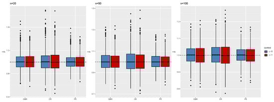
Figure 2. Distribution of the estimated $\beta$ from GMR, OR, and PR, $n=20,50,100$, $\alpha =0$, $\beta =1$, and $\gamma =0,1$.

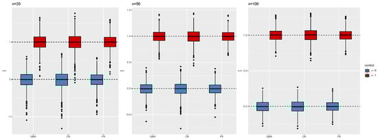
Figure 3. Distribution of the estimated $\gamma$ from GMR, OR, and PR, $n=20,50,100$, $\alpha =0$, $\beta =1$, and $\gamma =0,1$.

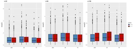
Figure 4. Distribution of the root mean squared error for the vector $\theta =(\alpha ,\beta ,\gamma )$ from GMR, OR, and PR, $n=20,50,100$, $\alpha =0$, $\beta =1$, and $\gamma =0,1$.

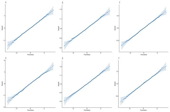
Figure 5. Normal QQ-plots from GMR, $n=100$, $\beta =1$, $\gamma =0$ (top), and $\gamma =1$ (bottom). The shaded area indicates 0.95-level confidence intervals.

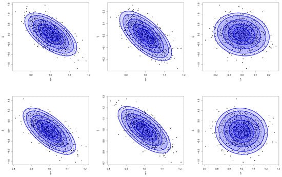
Figure 6. Paired joint distributions from GMR, $n=100$, $\beta =1$, $\gamma =0$ (top), and $\gamma =1$ (bottom). Gaussian contours overimposed for levels 0.25, 0.50, 0.75, 0.90, and 0.95.

Table 1. Empirical coverage of jackknife-based Wald-type confidence intervals for $\beta$, $n=20,50,100$, and nominal levels 0.90 and 0.95.

	GMR		PR		OR
	$\gamma =\mathbf{0}$
n	0.90	0.95	0.90	0.95	0.90	0.95
20	0.89	0.93	0.89	0.94	0.89	0.93
50	0.89	0.93	0.89	0.93	0.89	0.93
100	0.91	0.95	0.91	0.95	0.91	0.95
	$\gamma =1$
20	0.89	0.94	0.89	0.94	0.89	0.94
50	0.87	0.94	0.87	0.94	0.87	0.94
100	0.90	0.95	0.91	0.95	0.90	0.95

Table 2. Empirical coverage of jackknife-based Wald-type confidence regions for $(\alpha ,\beta )$, $n=20,50,100$, and nominal levels 0.90 and 0.95.

	GMR		PR		OR
	$\mathbf{\gamma }\mathbf{=}\mathbf{0}$
n	0.90	0.95	0.90	0.95	0.90	0.95
20	0.87	0.92	0.86	0.92	0.86	0.92
50	0.87	0.92	0.87	0.92	0.87	0.92
100	0.91	0.95	0.91	0.95	0.91	0.95
	$\gamma =1$
20	0.86	0.91	0.86	0.91	0.86	0.91
50	0.89	0.94	0.89	0.94	0.89	0.94
100	0.90	0.95	0.90	0.95	0.90	0.94

Table 3. Empirical coverage of jackknife-based Wald-type confidence regions for $(\beta ,\gamma )$, $n=20,50,100$, and nominal levels 0.90 and 0.95.

	GMR		PR		OR
	$\mathbf{\gamma }\mathbf{=}\mathbf{0}$
n	0.90	0.95	0.90	0.95	0.90	0.95
20	0.85	0.91	0.85	0.91	0.86	0.91
50	0.87	0.93	0.87	0.93	0.88	0.93
100	0.90	0.95	0.91	0.95	0.91	0.95
	$\gamma =1$
20	0.85	0.90	0.85	0.90	0.85	0.91
50	0.89	0.94	0.89	0.94	0.90	0.94
100	0.89	0.94	0.89	0.94	0.89	0.94

A second numerical experiment concerns data from the model in (13): the control variable is a dummy variable, based on which the sample is divided into equal sub-groups. The error structure is the same as above. We set $(\alpha ,{\beta }_1,{\beta }_2,\gamma )=(0,1,3,5)$. Figure 7 shows the negligible bias of the estimates for the intercept and slopes in the two groups, provided, respectively, by $(\alpha ,{\beta }_1)$ and $(\alpha +\gamma ,{\beta }_1+{\beta }_2)$ for all the considered symmetric regressions and sample sizes. Furthermore, we do not observe important differences between the methods in terms of RMSE, as displayed in Figure 8, meaning that GMR, PR, and OR still perform similarly, as expected under the simulation design involving constant and equal error variances. Table 4 provides empirical coverage of asymptotic Wald-type confidence intervals for the two slopes ${\beta }_1$ and ${\beta }_1+{\beta }_2$ and confidence regions for the pairs $(\alpha ,{\beta }_1)$ and $(\alpha +\gamma ,{\beta }_1+{\beta }_2)$ based on leave-one-out jackknife and the normal approximation. The results are quite satisfactory, with OR providing better results for inference on $(\alpha +\gamma ,{\beta }_1+{\beta }_2)$, in particular as the sample size grows.

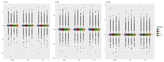
Figure 7. Distribution of the estimated intercept and slope for the first level of the covariate $(\alpha ,{\beta }_1)$ and the second level of the covariate $(\gamma ,{\beta }_1+{\beta }_2)$ from GMR, PR, OR, $n=20,50,100$, $\alpha =0$, ${\beta }_1=1$, ${\beta }_2=3$, and $\gamma =5$. Estimates are centered on the true values.

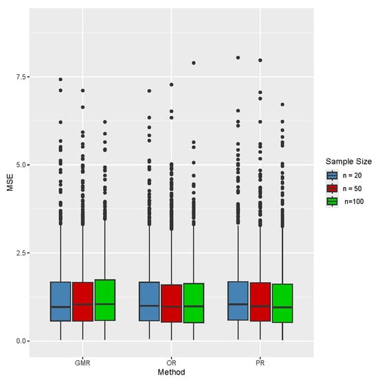
Figure 8. Distribution of the root mean squared error for the vector $\theta =(\alpha ,{\beta }_1,{\beta }_2,\gamma )$ from GMR, PR, and OR, $n=20,50,100$, $\alpha =0$, ${\beta }_1=1$, ${\beta }_2=3$, and $\gamma =5$, in the presence of one binary covariate and the interaction term.

Table 4. Empirical coverage of jackknife-based Wald-type confidence regions for $\alpha$, ${\beta }_1$, $(\alpha +\gamma )$, and $({\beta }_1+{\beta }_2)$ with $n=20,50,100$, and nominal levels 0.90 and 0.95 in the presence of one binary covariate and the interaction term.

		GMR		PR		OR
n		0.90	0.95	0.90	0.95	0.90	0.95
20	$\alpha$	0.82	0.92	0.88	0.92	0.88	0.91
	${\beta }_1$	0.82	0.87	0.81	0.86	0.82	0.87
	$\alpha +\gamma$	0.84	0.89	0.88	0.92	0.81	0.91
	${\beta }_1+{\beta }_2$	0.80	0.85	0.78	0.83	0.82	0.86
50	$\alpha$	0.89	0.93	0.90	0.93	0.89	0.93
	${\beta }_1$	0.85	0.91	0.85	0.91	0.85	0.91
	$\alpha +\gamma$	0.84	0.90	0.90	0.93	0.89	0.94
	${\beta }_1+{\beta }_2$	0.82	0.88	0.82	0.88	0.85	0.92
100	$\alpha$	0.91	0.95	0.91	0.95	0.91	0.95
	${\beta }_1$	0.87	0.93	0.87	0.93	0.87	0.93
	$\alpha +\gamma$	0.82	0.890	0.91	0.95	0.90	0.95
	${\beta }_1+{\beta }_2$	0.85	0.90	0.85	0.90	0.90	0.94

In summary, the key findings of the numerical studies are the satisfactory accuracy and precision of the proposed estimators under the different scenarios, and the fair reliability of associated inferences. We did not observe any remarkable differences between the symmetric regression methods under investigation.

4.2. Example: Reversible Conversion Formula for the HAQ and MDHAQ Scores

In rheumatology studies, the functional status of patients with inflammatory joint disease is typically measured using the Stanford Health Assessment Questionnaire (HAQ) disability score index [28]. The HAQ is composed of twenty items regarding eight domains of ability to perform activities of daily living: dressing and grooming, arising, eating, walking, hygiene, reach, grip, and activities. The overall score is obtained from averaging the domain scores and ranges from 0 to 3. However, it has been documented that filling out the HAQ can be time-consuming. To address this concern, a second score, the Multi-Dimensional HAQ (MDHAQ), has been suggested. The MDHAQ only includes eight of the original items from the HAQ, with the addition of two more items addressing some demanding activities that are considered to be more relevant. It also ranges from 0 to 3.

Based on these considerations, there is a practical need to establish a conversion formula between the two scores. The development of a conversion algorithm between the two scores has been pursued recently in [29] using data from the DANBIO, a Danish nationwide registry that includes all rheumatologic patients receiving biological drugs: demographic data, markers of disease activity, current treatment, adverse events, and reasons for discontinuation are registered at each visit. Since their methodology was based on OLS, we believe that a partial symmetric regression approach may be more suitable if the goal is to obtain a reversible conversion formula instead of two different formulas, as provided by classic linear regression. Like [29], we will use linear regression models despite the intrinsically discrete and bounded nature of HAQ and MDHAQ scores. Transformations that map the [0,3] interval to the real line may be considered to address the bounded nature of the data.

Our analysis is based on a sample of n = 43,522 patients from the DANBIO. We note that our sample size is much larger than the sample size of n = 13,391 from the study in [29]. The dataset contains the HAQ, MDHAQ, and age of the patient at the first visit where both HAQ and MDHAQ are available regardless of gender and diagnosis. Age is considered as a control variable when developing the conversion formula for the HAQ and MDHAQ scores. Summary statistics for the three variables are provided in Table 5. Their distributions are displayed in Figure 9: the relationship between the pair of measurements HAQ and MDHAQ is also illustrated in the bottom-right panel. We observe that the HAQ scores are larger on average than the MDHAQ scores. Looking at the quantiles, we notice that the distribution of the HAQ scores is shifted towards larger values compared to the distribution of the MDHAQ scores. There are not noticeable differences in variability. The bottom-right panel provides evidence supporting a linear relationship.

Table 5. Summary statistics for age, MDHAQ, and HAQ.

	Age	MDHAQ	HAQ
Minimum	15.00	0.0000	0.0000
1st Quartile	45.00	0.1000	0.1250
Median	58.00	0.4000	0.6250
Mean	56.42	0.5827	0.7333
3rd Quartile	69.00	0.9000	1.1250
Maximum	99.00	3.0000	3.0000
Standard Deviation	15.8814	0.5495	0.6773

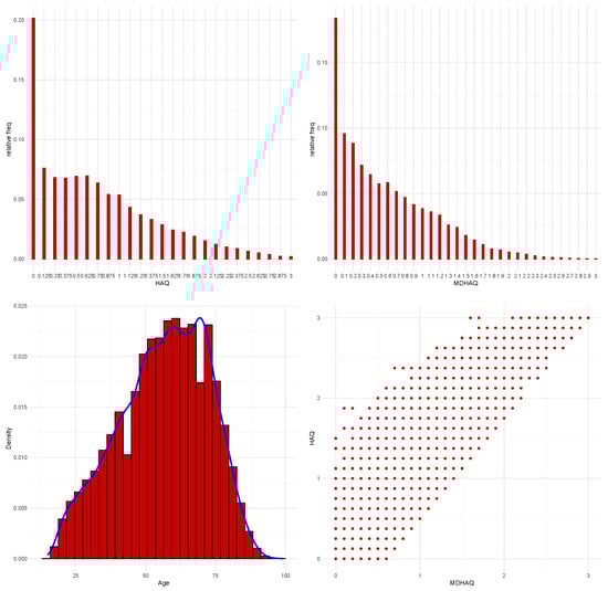
Figure 9. Distributions of HAQ, MDHAQ, age, and scatter-plot of the pairs of measurements regarding HAQ and MDHAQ.

In order to investigate the effect of age on the linear functional relationship of interest, let us consider the scatter-plot in Figure 10 describing the relationship between age and the difference between the HAQ and MDHAQ values. We observe that the differences in the scores tend to be larger as age increases. Then, it looks reasonable to obtain a conversion formula that also takes age into account.

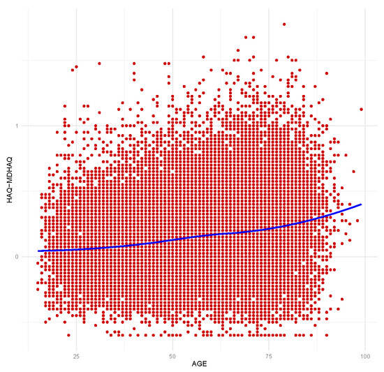
Figure 10. Scatter-plot of the differences in HAQ–MDHAQ measurements with age. Non-parametric trend line overimposed.

Since HAQ and MDHAQ scores have similar scale, we can use partial GMR. The fitted (reversible) conversion formula from MDHAQ to HAQ is

$$HAQ=-0.01142+1.2213MDHAQ+0.0024Age.$$

(14)

The estimates of the regression coefficients together with their standard errors (S.E.) are provided in Table 6. The other two methods, OR and PR, yielded almost identical results. The corresponding results from the OLS regression of HAQ on MDHAQ are also provided; estimates are biased because of measurement errors, and the corresponding conversion formula is not reversible. The reversible conversion formula from HAQ to MDHAQ is

$$MDHAQ=0.0935+0.8188HAQ-0.0020Age.$$

The estimate of the slope coefficient $\beta$ corresponding to MDHAQ in (14) is larger than one, as expected since on average the HAQ values are larger than the MDHAQ values. We also note that the estimate for the $\gamma$ coefficient corresponding to the control variable age is positive, as expected as well, based on the findings from Figure 10.

Table 6. Estimated coefficients and standard errors from the partial GMR and OLS regression.

	GMR		OLS
	Estimate	S.E.	Estimate	S.E.
$\alpha$	−0.1142	0.0047	−0.0795	0.0049
$\beta$	1.2213	0.0024	1.1137	0.0024
$\gamma$	0.0024	0.0001	0.0029	0.0001

5. Discussion

In this work, we introduced a partial symmetric linear regression model aimed at describing a reliable conversion formula between error-prone measurements in the presence of control variables, which are assumed to be known without error. The extension to partial settings with control variables fills a notable gap in the literature. This approach can be tested in applied domains where parallel measurement tools coexist, such as psychology, health economics, or epidemiology. More generally, symmetric regression could prove to be highly relevant in interdisciplinary fields that rely heavily on measurement harmonization, including environmental science and social research.

The proposed model enables studying the effect of control variables on the functional relationship between a set of variables in terms of their statistical equivalence and practical interchangeability to take into account confounding influences. Compared to classical regression approaches, the proposed methodology offers important advancements by producing reversible mappings and appropriately accounting for measurement error. Partial symmetric regression provides a flexible and powerful tool for enhancing the comparability of measurements across diverse scientific fields. Attention was focused on very popular strategies for symmetric regression, such as OR, GMR, and PR. Model fitting was achieved through the minimization of a suitable objective function that is derived by generalizing the methodology used for symmetric regression to the case when control variables are considered. The key element is that the objective function is based on a suitable summary measure of the squared errors concerning the $(Y,\mathbf{X})$ variables, whose reversible conversion formula is of primary interest, but not the control variables $\mathbf{Z}$. In detail, GMR is based on the geometric mean of squared errors, PR on the arithmetic mean, and OR on the harmonic mean.

The proposed methodology performed well both in the numerical studies and the empirical application taken from rheumatology. The numerical investigations, described in Section 4.1, provide evidence supporting the reliability of the proposed partial symmetric regression methodology and the accuracy of the related statistical inference. Across a range of simulated scenarios, the estimators displayed negligible bias and satisfactory efficiency. In particular, the empirical coverage of Wald-type confidence intervals and regions consistently matched the nominal level, especially as the sample size increased. These results support the asymptotic theory underlying the estimators and reinforce the practical utility of the new methodology. The observed similarity between the results from the geometric mean regression, orthogonal regression, and Pythagorean regression further suggests that the methodology is not unduly sensitive to the choice of the symmetric regression variant, at least for the settings considered in our study.

The application to rheumatology data, discussed in Section 4.2, illustrates the potential of the new methodology to deliver practically meaningful results. The construction of a reversible conversion formula between the HAQ and MDHAQ scores represents more than a theoretical result: it addresses a substantive clinical need as reversible and statistically consistent mappings between patient-reported outcomes are indispensable for harmonizing research evidence and facilitating longitudinal monitoring across studies and registries. The inclusion of age as a control variable not only improved the fidelity of the conversion but also highlighted the role of demographic heterogeneity when dealing with patient-reported outcomes.

From a methodological perspective, our findings resonate with calls [30] to prioritize models that respect measurement error structures and yield interpretable invertible relationships between paired measurements or instruments. As such, this study opens promising avenues for both theoretical developments and practical applications. At the same time, some limitations should be acknowledged. First, while the numerical studies were comprehensive in their scope, they necessarily relied on simplified data-generating mechanisms. Second, while partial symmetric regression provides reversibility, its reliance on linear functional forms may prove to be restrictive when the true relationships between variables are nonlinear. Looking ahead, it would be valuable to extend the present framework to accommodate nonlinear symmetric regression structures [31] as a possible direction for future research. A Bayesian extension may also enhance uncertainty quantification and facilitate the inclusion of prior information [32].

References

- Taagepera, R. Making Social Sciences More Scientific: The Need for Predictive Models; Oxford University Press: Oxford, UK, 2008. [Google Scholar]
- Carr, J.R. Orthogonal regression: A teaching perspective. Int. J. Math. Educ. Sci. Technol. 2012, 43, 134–143. [Google Scholar] [CrossRef]
- Francq, B.G.; Govaerts, B.B. Measurement methods comparison with errors-in-variables regressions. From horizontal to vertical OLS regression, review and new perspectives. Chemom. Intell. Lab. Syst. 2014, 134, 123–139. [Google Scholar] [CrossRef]
- Greco, L.; Luta, G.; Krzywinski, M.; Altman, N. Symmetric alternatives to the ordinary least squares regression. Nat. Methods 2025, 22, 1610–1612. [Google Scholar] [CrossRef] [PubMed]
- Chen, A.; Bengtsson, T.; Ho, T.K. A Regression Paradox for Linear Models: Sufficient Conditions and Relation to Simpson’s Paradox. Am. Stat. 2009, 63, 218–225. [Google Scholar] [CrossRef]
- Pearson, K. On lines and planes of closest fit to systems of points in space. London, Edinburgh, Dublin Philos. Mag. J. Sci. 1901, 2, 559–572. [Google Scholar] [CrossRef]
- Adcock, R.J. A problem in least squares. Analyst 1878, 5, 53–54. [Google Scholar] [CrossRef]
- Adcock, R. Extension of the method of least squares to any number of variables. Analyst 1880, 7, 22–23. [Google Scholar] [CrossRef]
- Stromberg, G. Accidental and Systematic Errors in Spectroscopic Absolute Magnitudes for Dwarf G0-K2 Stars. Astrophys. J. 1940, 92, 156. [Google Scholar] [CrossRef]
- Kermack, K.; Haldane, J.B. Organic correlation and allometry. Biometrika 1950, 37, 30–41. [Google Scholar] [CrossRef]
- Xu, S. A property of geometric mean regression. Am. Stat. 2014, 68, 277–281. [Google Scholar] [CrossRef]
- Greene, N. Generalized Least Squares Regression I: Efficient derivations. In Proceedings of the 1st International Conference on Computational Science and Engineering, Valencia, Spain, 6–8 August 2013. [Google Scholar]
- Deming, W.E. Statistical Adjustments of Data; Dover Publications: New York, NY, USA, 1943. [Google Scholar]
- Ripley, B.D.; Thompson, M. Regression techniques for the detection of analytical bias. Analyst 1987, 112, 377–383. [Google Scholar] [CrossRef]
- Linnet, K. Estimation of the linear relationship between the measurements of two methods with proportional errors. Stat. Med. 1990, 9, 1463–1473. [Google Scholar] [CrossRef] [PubMed]
- Carroll, R.J.; Ruppert, D.; Stefanski, L.A.; Crainiceanu, C.M. Measurement Error in Nonlinear Models: A Modern Perspective; Taylor & Francis Group: Abingdon, UK, 2006. [Google Scholar]
- Fuller, W.A. Measurement Error Models; John Wiley & Sons: Hoboken, NJ, USA, 2009. [Google Scholar]
- Kim, T.; Luta, G.; Bottai, M.; Chausse, P.; Doros, G.; Pena, E.A. Maximum Agreement Linear Prediction via the Concordance Correlation Coefficient. arXiv 2023, arXiv:2304.04221. [Google Scholar]
- Tan, C.Y.; Iglewicz, B. Measurement-methods comparisons and linear statistical relationship. Technometrics 1999, 41, 192–201. [Google Scholar] [CrossRef]
- Greene, N. Generalized Least-Squares Regressions V: Multiple Variables. In New Developments in Pure and Applied Mathematics, Proceedings of the International Conference on Mathematical Methods, Mathematical Models and Simulation in Science and Engineering (MMSSE 2015), Vienna, Austria, 15–17 March 2015; INASE: London, UK, 2015. [Google Scholar]
- Isobe, T.; Feigelson, E.D.; Akritas, M.G.; Babu, G.J. Linear regression in astronomy. Astrophys. J. 1990, 364, 104–113. [Google Scholar] [CrossRef]
- Stefanski, L.A.; Boos, D.D. The calculus of M-estimation. Am. Stat. 2002, 56, 29–38. [Google Scholar] [CrossRef]
- Kelly, G. The influence function in the errors in variables problem. Ann. Stat. 1984, 12, 87–100. [Google Scholar] [CrossRef]
- Gillard, J.; Iles, T. Variance Covariance Matrices for Linear Regression with Errors in Both Variables; Cardiff University School of Mathematics Technical Report; Cardiff University: Cardiff, UK, 2006. [Google Scholar]
- Therneau, T. deming: Deming, Theil-Sen, Passing-Bablock and Total Least Squares Regression, R package version 1.4; R Foundation for Statistical Computing: Vienna, Austria, 2018. [Google Scholar]
- Francq, B.G. Bootstrap in Errors-in-Variables Regressions Applied to Methods Comparison Studies. Inform. Medica Slov. 2014, 19, 1. [Google Scholar]
- Potapov, S.; Model, F.; Schuetzenmeister, A.; Manuilova, E.; Dufey, F.; Raymaekers, J. mcr: Method Comparison Regression, R package version 1.3.3.1; R Foundation for Statistical Computing: Vienna, Austria, 2024. [Google Scholar]
- Fries, J.F. The dimension of health outcomes: The Health Assessment Questionnaire. J. Rheumatol. 1982, 9, 789–793. [Google Scholar]
- Ørnbjerg, L.M.; Svensson, E.; Løngaard, K.; Meincke, R.H.; Pedersen, J.K.; Dreyer, L.; Krogh, N.S.; Jensen, D.V.; Hetland, M.L. Conversion of the MDHAQ to the HAQ score: A simple algorithm developed and validated in a cohort of 13 391 real-world patients. Rheumatology 2022, 61, 3919–3929. [Google Scholar] [CrossRef]
- Li, M.; Ma, Y. An update on measurement error modeling. Annu. Rev. Stat. Its Appl. 2024, 11, 279–296. [Google Scholar] [CrossRef]
- Barry, T.; Roeder, K.; Katsevich, E. Exponential family measurement error models for single-cell CRISPR screens. Biostatistics 2024, 25, 1254–1272. [Google Scholar] [CrossRef]
- Ma, Z.; Chen, M.H. A Bayesian model-based reduced major axis regression. Biom. J. 2024, 66, 2300279. [Google Scholar] [CrossRef]
Disclaimer/Publisher’s Note: The statements, opinions and data contained in all publications are solely those of the individual author(s) and contributor(s) and not of MDPI and/or the editor(s). MDPI and/or the editor(s) disclaim responsibility for any injury to people or property resulting from any ideas, methods, instructions or products referred to in the content. |
© 2025 by the authors. Licensee MDPI, Basel, Switzerland. This article is an open access article distributed under the terms and conditions of the Creative Commons Attribution (CC BY) license (https://creativecommons.org/licenses/by/4.0/).