Passenger Flow-Oriented Operating Period Division in Urban Rail Transit: A Hybrid SOM and K-Means Clustering Approach

Abstract

The accurate division of operating periods in urban rail transit (URT) is crucial for reasonable scheduling. However, the current determination of operating breakpoints largely relies on the empirical judgment of operators, and symmetric period schemes are usually adopted, which fail to effectively reflect the uneven temporal distribution of passenger flow across different lines and directions. This study proposes a hybrid SOM–K-means framework for dividing daily operating periods based on automatic fare collection (AFC) data, the method extracts features from three dimensions of passenger flow, total volume, microscopic fluctuations and macroscopic distribution. A case study is conducted based on data from Tianjin URT Lines 1 and 2. The results demonstrate that the clustering-based operating period division effectively reveals transition periods between peak and off-peak hours, as well as late-night periods that are not captured by the existing scheme, while also reflecting temporal asymmetry across lines and directions. Consequently, compared to current schemes, this division offers a more accurate representation of passenger flow characteristics, enhancing the precision of scheduling work and operational efficiency. Moreover, the SOM–K-means method shows robust clustering performance and stability across various scenarios and sample sizes. This study offers insights for URT to achieve refined scheduling and demand-responsive operations based on passenger flow.

1. Introduction

With the rapid expansion of urban areas, urban rail transit (URT) has become an increasingly essential component of public transportation. It plays a key role in addressing rising travel demands, easing surface traffic congestion, and mitigating environmental pollution from vehicular emissions [1,2]. In large metropolitan areas, URT, characterized by high service frequency and dense operational intensity, effectively accommodates the massive commuting demand on weekdays and has evolved into the backbone of the urban public transportation system [3,4]. However, due to factors such as urban spatial planning, network topology, and the diversity of passenger travel behaviors, URT exhibit pronounced temporal heterogeneity in passenger demand patterns. To ensure operational efficiency and achieve the optimal allocation of limited transit resources, train operation schemes must be flexibly adjusted in accordance with the temporal dynamics of passenger demand. A widely adopted strategy in practice is to divide the service day into multiple distinct times (e.g., peak and off-peak hours [5,6,7]), within which key scheduling parameters, such as headways, train allocations, and travel times, are adjusted according to anticipated demand. Hence, accurate division of operating periods underpins demand-responsive strategies in URT, supporting timetable optimization, crew scheduling, and station-level resource allocation.

However, in practical applications, the division of operational periods often relies heavily on the subjective judgment of operators [8,9], which is typically based on limited experience or imprecise analyses of passenger demand data [10]. A common approach is to depict the temporal distribution of total passenger flow throughout the day and manually determine period breakpoints based on significant changes in passenger flow [10]. Such practices give rise to two main issues. First, subjective factors may lead to inappropriate period divisions; second, passenger flow volume alone cannot comprehensively capture the multidimensional characteristics of passenger demand. Moreover, influenced by urban planning and development, different lines within the URT network undertake distinct spatial functions and serve varying areas. Consequently, the intensity, temporal distribution, and variation patterns of passenger demand often differ significantly across lines and directions. For instance, on lines connecting suburban districts and the urban areas, passenger flows predominantly move toward downtown during the day, whereas in the evening, the reverse flow toward the suburbs becomes more pronounced [11], resulting in evident temporal asymmetry in passenger flow between the two directions of the same line. Operators often employ a unified time-period segmentation strategy across the entire network or apply symmetric operational time arrangements, assigning identical peak and off-peak periods to both directions of the same line. Such practices may obscure the intrinsic differences in passenger flow characteristics and fail to capture the spatiotemporal complexity and variability of passenger demand, which arise from variations in passengers’ departure time preferences, route choices, and commuting regularities. The supply of train capacity should be precisely matched with passenger travel demand to achieve the rational allocation of resources. For directions with high passenger volumes, higher train departure frequencies should be implemented to accommodate concentrated travel demand, whereas for directions with lower demand, operating at lower frequencies can still ensure an adequate level of service quality. Furthermore, the time windows of high- and low-demand passenger flows differ across lines and travel directions. Therefore, applying a unified operating period scheme and corresponding departure frequency may lead to either excess or insufficient capacity, directly affecting the operational efficiency and cost of urban rail transit systems.

Consequently, relying on empirical judgment and uniform division impedes the ability of URT to accurately respond to dynamic passenger demand patterns and undermines the precision and efficiency of resource allocation. Passenger flow analysis methods based on macroscopic statistics are limited in their ability to comprehensively characterize the spatiotemporal distribution of passenger demand and to accurately identify its asymmetry. The widespread deployment of automated fare collection (AFC) systems has enabled the acquisition of large-scale, high-resolution passenger flow data, providing new opportunities for refined, data-driven operational planning in URT. In this context, it is imperative to develop robust methodologies capable of handling diverse and dynamically changing passenger flow patterns while precisely dividing operational periods.

Although prior studies have explored data-driven approaches for operating period division—such as time series clustering [12], hierarchical clustering [13,14], and optimization-based breakpoint detection [15]—several challenges remain in their practical application to URT. Time-series clustering methods are often constructed based solely on passenger flow features or statistical measures derived from passenger flow [12,16], thereby neglecting the multi-dimensional nature of passenger demand. Fisher’s least squares partition algorithm [17] is commonly employed in time-series clustering. Preserving the temporal order during clustering, however, renders the results highly sensitive to outliers and thus susceptible to noise. Hierarchical clustering, which is not constrained by temporal ordering, evaluates similarity between samples using inter-sample distances [18], and has been applied to problems such as intersection signal timing optimization [13] and the division of bus operation periods [14]. Nevertheless, its performance often deteriorates when dealing with datasets characterized by complex structures [19]. Heuristic-based clustering methods for operating period division are essentially optimization problems, in which the quality of the clustering results depends strongly on the choice of model and algorithm, and they are prone to becoming trapped in local optima. In contrast, K-means provides relatively high computational efficiency and a certain degree of interpretability, making it suitable for clustering multi-dimensional time-period samples [9]. However, its performance depends largely on the initialization of the centroid. When dealing with high-dimensional data characterized by strong fluctuations and non-spherical clusters, K-means often produces suboptimal results. Moreover, the clustering results should not only reflect the effectiveness of period division but also ensure practical interpretability and robustness. This allows the results to remain consistent and rational even in the presence of noise and data fluctuations, thereby improving the reliability of operational management.

To address these limitations, this study employs a hybrid SOM–K-means approach. The self-organizing map (SOM) is a type of feedforward neural network whose primary advantage lies in its ability to map high-dimensional input data onto a low-dimensional (typically two-dimensional) grid, thereby enabling intuitive visualization of clustering results. During this process, SOM generates a set of prototype vectors (i.e., weight vectors) that characterize the distribution of the original sample data. Each prototype vector represents the local average of neighboring samples, effectively smoothing out random noise in the original data [20]. Previous studies have demonstrated that SOM exhibits strong robustness when clustering data containing noise [21,22,23]. When clustering operational periods based on passenger travel data derived from AFC systems, the inherent randomness of passenger demand may introduce noise into the sample data, thereby hindering the accurate identification of cluster boundaries and reducing the stability and reliability of clustering results. Moreover, relying solely on passenger flow volume is insufficient to comprehensively capture the behavioral characteristics and latent patterns of passenger demand. Therefore, constructing a multidimensional feature framework is essential for a more holistic representation of passenger flow samples and for achieving operational period segmentation that more accurately aligns with actual demand.

Benefiting from the superior clustering performance and robustness of SOM in handling multidimensional noisy data, this study employs SOM for pre-clustering the original passenger flow samples, effectively filtering out noise and smoothing the raw data. However, the number of clusters generated by SOM is often substantially higher than the actual number required, making the pre-clustering results difficult to directly translate into operationally meaningful period divisions, thereby reducing the interpretability of the clustering outcomes. To address this limitation, K-means is employed as a post-processing step to refine the initial SOM clusters, thereby enhancing their interpretability and applicability for operational period division. Such a two-stage clustering framework has been shown to be more effective in identifying potential data partitions and enhancing the interpretability of clustering outcomes [23]. Nevertheless, most existing studies on the SOM–K-means approach have largely overlooked the potential risk of convergence to local optima caused by the random initialization of K-means centroids [24,25,26], which compromises the stability of clustering outcomes and poses challenges to obtaining consistent operational period divisions in practice. To overcome this issue, a small-scale SOM network is specifically designed in this study to initialize the K-means cluster centers, significantly improving the stability and accuracy of the final results by mitigating the uncertainties associated with random initialization.

To evaluate the effectiveness of this framework, a case study utilizing real-world AFC data from the Tianjin Rail Transit is conducted. The main contributions of this study include:

• This study establishes a novel multi-dimensional time-period sample space that incorporates total volume, microscopic variations, and macroscopic distribution of passenger flow. Unlike previous studies that constructed clustering samples solely based on total passenger flow [8,12,16], the proposed framework captures passenger flow characteristics more comprehensively, thereby providing finer insights into passenger travel demand.
• To address the limitations of conventional single clustering methods [12,13,14] in processing multi-dimensional and noisy passenger flow data, this study proposes a hybrid self-organizing map (SOM)–K-means framework. The SOM is employed to pre-cluster the original sample data, effectively filtering and smoothing noise [20]. Subsequently, the K-means refines and merges the preliminary clusters to generate final clusters with improved interpretability and practical applicability. Moreover, a small-scale SOM network is specifically designed to initialize K-means centroids, mitigating the uncertainty associated with random initialization and enhancing the robustness and accuracy of URT operational period division. Notably, this improvement has been largely overlooked in previous studies employing the SOM–K-means framework [24,25,26].
• In contrast to prior studies that predominantly examine a single line or travel direction [8,9,12], this study employs real-world URT passenger travel data to empirically reveal the intrinsic asymmetry of operational periods across different lines and travel directions, driven by heterogeneous passenger demand structures and spatiotemporal distribution patterns. The findings verify the effectiveness and applicability of the proposed method in supporting fine-grained operational management.

The remainder of this paper is organized as follows. Section 2 reviews the related literature. Section 3 describes the construction of the sample space in detail. Section 4 introduces the SOM–K-means clustering framework. Section 5 presents a case study on Tianjin Rail Transit Lines 1 and 2 to validate the effectiveness of the proposed hybrid clustering method. Finally, Section 6 concludes the main findings and discusses directions for future work.

2. Literature Review

Research on operating period division in the transportation domain originated from studies on optimizing time-of-day (TOD) signal timing plans. Smith et al. [13] applied hierarchical clustering to traffic flow and occupancy data collected via intelligent transportation system sensors, determining optimal breakpoints for adaptive signal timing. Similarly, Park et al. [27] used historical traffic volume data and a genetic algorithm to dynamically determine time breakpoints, reducing total intersection delays. Chen et al. [28] compared K-means, hierarchical clustering, and Fisher’s ordered clustering on directional traffic volume samples, finding that Fisher’s method delivered superior performance in minimizing control delay, queue length, and stop frequency, offering a more nuanced and responsive TOD segmentation framework. These studies typically focus on a single feature—traffic volume—and construct relatively simple sample structures, allowing classical clustering algorithms to efficiently process the data and achieve satisfactory clustering results.

Parallel research in public bus transit has focused on timetable formulation and service reliability. Salicrú et al. [14] introduced a hierarchical classification algorithm to segment daily operating hours, enabling more punctual and demand-responsive timetables. Bie et al. [10] analyzed GPS-based dwell times and travel times to establish segmentation thresholds for daily operations. Mendes-Moreira et al. [29] applied decision tree methodologies to identify recurring daily operational patterns throughout the year. This enabled the generation of stratified timetables better aligned with seasonal variations in travel demand. In another notable contribution, Shen et al. [30] refined K-means centroid initialization and distance metrics to achieve more accurate segmentation of daily service hours using one-way trip time as the core feature vector. Jin et al. [15] further extended this line of research by integrating multi-source data, such as passenger demand and vehicle operational data into an optimization model. Their work employed a genetic algorithm to determine optimal segmentation breakpoints aimed at minimizing fleet operating costs, offering a more holistic perspective that considers both service provision and resource efficiency. Overall, in studies on dividing bus operating period, time-period samples have been constructed using multi-dimensional features, and clustering algorithms suitable for high-dimensional data have increasingly attracted attention. Nevertheless, these studies remain limited in capturing the temporal dynamics of passenger flow or traffic volume.

Compared with studies in the contexts of bus systems and traffic signal control, research on URT operating period division remains relatively limited. Existing studies have primarily focused on constructing time samples by extracting features from inbound passenger volumes or sectional flows between adjacent stations and then applying clustering-based methods to group periods with similar passenger flow characteristics. For instance, Zeng et al. [12] constructed unidirectional OD probability matrices based on intra-period passenger flow data and applied an ordered sample clustering method, incorporating similar interstation-passenger-transfer rules to generate operational period divisions. Although this approach accounts for the spatial transfer characteristics of passenger flows, the sample features are primarily based on statistical metrics of flow volume and fail to adequately capture the temporal dynamics of passenger demand. Wang et al. [8] constructed time samples using inbound passenger volumes and employed the affinity propagation algorithm to cluster and merge samples with similar characteristics. The optimized division of operating periods significantly reduced the average passenger waiting time. However, the study relied solely on inbound volumes, which provides an incomplete representation of dynamic passenger demand across periods. Chen et al. [9] constructed a feature set comprising six indicators—including the maximum, minimum, mean, standard deviation, and rise/fall time ratios of passenger volume—to characterize the temporal patterns of passenger flow. Subsequently, the K-means clustering algorithm was employed to merge representative periods, resulting in a more refined operational period division scheme. However, the constructed samples primarily reflect prominent trends in passenger flow variation and do not provide quantitative measures of intra-period variability. In addition, the robustness and stability of K-means clustering when applied to multi-dimensional feature sets remain unexamined. Tang et al. [16] emphasized the pronounced spatiotemporal heterogeneity of URT passenger flows and proposed an ordered clustering method that integrates both temporal dynamics and spatial distribution characteristics. The resulting clusters exhibit strong interpretability and practical applicability, significantly enhancing the accuracy of operating period division. While the present approach better accounts for variations across space and time, it still relies on sectional flows as the primary feature, thereby neglecting other critical dimensions of passenger demand, such as intra-period variability.

Although the aforementioned studies have laid a foundation for dividing operational periods in URT, several limitations remain to be addressed: (1) they primarily focus on single-dimensional features of passenger flow, neglecting intra-period dynamics, which may result in divisions that inadequately reflect actual passenger demand; (2) single clustering algorithms exhibit limited stability when handling multi-dimensional and noisy data. Algorithms such as K-means, affinity propagation algorithm, and ordered sample segmentation algorithm mainly rely on sample distance variations during clustering, rendering the results highly sensitive to outliers. However, the stability of cluster outcomes has been largely overlooked in previous studies; (3) most existing research concentrates on individual lines or travel directions, lacking systematic validation of the proposed methods across different lines or directions in the URT network. Notably, the potential asymmetry of operational periods among different lines or travel directions remains largely unexplored.

To address these research gaps, this study first constructs a multi-dimensional feature indicator system for time samples in terms of three dimensions of passenger flow: total volume, microscopic fluctuation, and macroscopic distribution, thereby overcoming the limitations of prior studies that relied solely on passenger volume. Second, a hybrid SOM–K-means clustering framework is proposed to effectively handle high-dimensional, noisy data, attenuate the influence of outliers, and ensure robust and stable clustering outcomes. Third, the scope of the analysis is extended across multiple lines and directions of URT, revealing inherent asymmetries in operational period schemes.

3. Construction of Sample Space

3.1. Data Source

The AFC system has been widely implemented in the daily operations of URT. As a key component of intelligent transportation infrastructure, the AFC automatically records passenger travel information when passengers swipe their cards at station gates. The recorded data includes entry and exit stations and their corresponding timestamps. Compared to traditional survey methods, AFC data offers substantial advantages in both volume and accuracy. These advantages make it particularly suitable for describing and analyzing the spatiotemporal characteristics of passenger flows. In this study, multi-day AFC passenger travel records are used to construct the clustering sample space. The raw dataset $E$ for cluster analysis is presented in Equation (1).

$$E=\left(\begin{array}{ccccc}{e}_1^1& \cdots & e_1^j& \cdots & e_1^M\\ ⋮& \ddots & ⋮& \ddots & ⋮\\ e_i^1& \cdots & e_i^j& \cdots & e_i^M\\ ⋮& \ddots & ⋮& \ddots & ⋮\\ e_N^1& \cdots & e_N^j& \cdots & e_N^M\end{array}\right)$$

(1)

where $e_i^j$ represents the i-th data collected on the day $j$. Here, $M$ denotes the total number of days covered by the AFC data used in this study, and $N$ indicates the total amount of raw data.

Commuters constitute an important component of URT passengers [31,32], and their daily commuting behavior largely influences the spatiotemporal distribution of passenger flow. Weekdays represent the main operational scenario of urban rail transit, and the division of operational periods needs to align with the travel demand of commuting passengers in order to enhance service quality and achieve efficient allocation of transportation resources. Therefore, this study focuses on the division of operational periods during commuting hours (i.e., weekdays).

A total of 2,723,650 historical passenger travel records were extracted from the Tianjin URT AFC system, covering both upstream and downstream directions of the Lines 1 and 2 over five consecutive weekdays (13–17 December 2021), with $M=5$ representing the number of days in the raw dataset $E$. The dataset captures passenger transactions at all stations on both lines spanning the entire service period, from the first train departure to the termination of the last train service, at a 1 min resolution.

3.2. Feature Selection

Each time sample in the sample space exhibits distinct characteristics. During clustering, samples with similar characteristics are grouped into the same category, typically corresponding to the same time in the results. Relying solely on passenger flow volumes is insufficient to capture the variations in flow dynamics across different times. To comprehensively capture the spatiotemporal characteristics of passenger flow, this study employs nine feature indicators, including the maximum, minimum, and average values of passenger volumes; the maximum, minimum, and average values of passenger volume changes between adjacent time intervals; and the ranking positions of the aforementioned three passenger volume indicators within the full-day sample. The ranking positions are determined based on the magnitude of each indicator in the full-day dataset, with larger values assigned higher ranks. These indicators collectively describe the passenger flow characteristics within each time sample in terms of total volume, microscopic variations, and macroscopic distribution.

3.2.1. Passenger Flow Total Volume

Maximum passenger flow refers to the highest number of passengers that the URT is required to transport during a given sample time. This indicator can be obtained from Equation (2).

$$p_{i,\max }=\max \left\{p_i^1,p_i^2,\cdots ,p_i^M\right\},i=1,2,\cdots ,n$$

(2)

where $p_i^M$ represents the total passenger flow of the i-th sample collected on day $M$, including passengers entering and exiting at stations. $n$ represents the number of samples.

Minimum passenger flow represents the lower bound of the number of passengers served by the URT within a sample time. Similarly, this indicator can be derived using Equation (3).

$$p_{i,\min }=\min \left\{p_i^1,p_i^2,\cdots ,p_i^M\right\},i=1,2,\cdots ,n$$

(3)

Average passenger flow represents the overall ridership intensity of the URT during a sample time period. This indicator can be calculated using Equation (4).

$$p_{i,avg}={\displaystyle \frac{{\displaystyle \sum _{j=1}^M{p}_i^j}}{M}},i=1,2,\cdots ,n$$

(4)

3.2.2. Passenger Flow Microscopic Fluctuations

This study characterizes the dynamic fluctuations in passenger flow using per-minute changes. Specifically, the change rate of passenger flow at each minute relative to the previous minute is first calculated for each day, and then the results over five consecutive working days are aggregated to form the sample features used for clustering analysis.

Since the first sample lacks a value for the rate of change in passenger flow, only the samples from the second to the n-th are included in the clustering and dividing process. To preserve temporal continuity in the clustering results, the first sample is subsequently assigned to the same time period as the second sample.

Maximum change in passenger flow represents the largest positive fluctuation during passenger flow variations. This indicator is especially important during peak periods for identifying pre-peak phases and can be calculated using Equation (5).

$$c_{i,\max }=\underset{j\in \left\{1,2,\cdots ,M\right\}}{\max }\left\{{\displaystyle \frac{p_i^j-p_{i-1}^j}{\max \left(p_{i-1}^j,\epsilon \right)}}\right\}, i=2,3,\cdots ,n$$

(5)

where $\epsilon$ is a small positive constant added to prevent division by 0. In this study, $\epsilon$ is set to 1, representing the smallest passenger flow unit.

Minimum change in passenger flow refers to the largest negative fluctuation during the variation process of passenger flow. Similarly, this metric helps identify the post-peak hours following peak periods and can be calculated using Equation (6).

$$c_{i,\min }=\underset{j\in \left\{1,2,\cdots ,M\right\}}{\min }\left\{{\displaystyle \frac{p_i^j-p_{i-1}^j}{\max \left(p_{i-1}^j,\epsilon \right)}}\right\}, i=2,3,\cdots ,n$$

(6)

Average change in passenger flow reflects the overall trend of variation within the time sample. For computational convenience, this indicator is calculated using Equation (7).

$$c_{i,avg}=\left\{{\displaystyle \frac{p_{i,avg}^j-p_{i-1,avg}^j}{\max \left(p_{i-1,avg}^j,\epsilon \right)}}\right\}, i=2,3,\cdots ,n$$

(7)

3.2.3. Passenger Flow Macroscopic Distribution

Passenger flow distribution characterizes the aggregation patterns of URT passenger flow throughout the entire daily operational period. In this study, the indicator is defined based on the ranking of current sample’s passenger flow within all samples, which eliminates the influence of absolute values of passenger flow. Meanwhile, the adoption of rank effectively limits zero-value occurrences, mitigating their potential impact on clustering results. This feature indicator can be calculated using Equations (8)–(10).

$$r_{i,\max }=1+{\displaystyle \sum _{l=1}^n\mathbf{1}\left[p_{l,\max }>p_{i,\max }\right]}$$

(8)

$$r_{i,\min }=1+{\displaystyle \sum _{l=1}^n\mathbf{1}\left[p_{l,\min }>p_{i,\min }\right]}$$

(9)

$$r_{i,avg}=1+{\displaystyle \sum _{l=1}^n\mathbf{1}\left[p_{l,avg}>p_{i,avg}\right]}$$

(10)

where $\mathbf{1}\left[\right]$ is the indicator function. The function returns a value of 1 if the condition in brackets is satisfied; otherwise, it returns 0.

In summary, the constructed sample space is mathematically defined in Equation (11).

$$S=\left[\begin{array}{c}{s}_1\\ ⋮\\ s_{n-1}\end{array}\right]=\left[\begin{array}{ccccccccc}{p}_{1,\max }& p_{1,\min }& p_{1,avg}& c_{1,\max }& c_{1,\min }& c_{1,avg}& r_{1,\max }& r_{1,\min }& r_{1,avg}\\ ⋮& ⋮& ⋮& ⋮& ⋮& ⋮& ⋮& ⋮& ⋮\\ p_{n-1,\max }& p_{n-1,\min }& p_{n-1,avg}& c_{n-1,\max }& c_{n-1,\min }& c_{n-1,avg}& r_{n-1,\max }& r_{n-1,\max }& r_{n-1,avg}\end{array}\right]$$

(11)

4. Methodology

4.1. SOM–K-Means

The SOM is a type of feedforward neural network and belongs to the category of unsupervised learning algorithms [33]. The core principle of the algorithm originates from the lateral inhibition phenomenon observed in biological neural systems: when the system is stimulated, different regions respond according to the stimulation pattern. The activated neuron inhibits its neighboring neurons and emerges as the winner through a competitive process. Based on this mechanism, SOM can be used to detect latent features in sample data and cluster similar data accordingly.

SOM is capable of learning features from high-dimensional data and projecting them onto a low-dimensional space while largely preserving the original topological relationships [34], thereby enabling intuitive visualization. However, SOM has inherent limitations. Its neuron activation and adjustment processes are highly sensitive to the order of sample inputs. During training, slight changes in the sequence may cause similar samples to activate different neurons, potentially resulting in their assignment to different clusters and thus compromising the accuracy of the clustering results. Additionally, when applied to large-scale datasets, SOM often requires a large number of neurons, which can result in over-segmentation and reduced interpretability—an undesirable outcome in practical decision-making contexts, where fewer, more concise clusters are preferred [24].

K-means is a classical unsupervised clustering algorithm known for its simplicity, fast convergence, and easily interpreted results [35]. It requires minimal hyperparameter tuning, with only the number of clusters needing to be specified. However, the algorithm minimizes the sum of squared distances between samples and their corresponding cluster centroids through iterative optimization. As a result, its performance is highly sensitive to the initial selection of centroids, particularly in high-dimensional spaces where data sparsity can exacerbate randomness in initialization. This often leads to unstable and less accurate clustering results.

To fully leverage the complementary strengths of the two algorithms, this study proposes a hybrid SOM–K-means clustering framework. Initially, the SOM is employed to perform preliminary clustering of high-dimensional samples, based on which a dissimilarity matrix is constructed. A small-scale SOM network is then built, with the number of neurons set to $k$. The weight vectors of the trained SOM neurons are used as the initial centroids for the K-means, thereby reducing sensitivity to initialization and enhancing clustering stability. Subsequently, the dissimilarity matrix is used as input to the K-means, and the optimal number of clusters $k$ is determined using the Davies–Bouldin Index (DBI) [36], ensuring a more reasonable dividing of the sample space. Finally, the K-means is applied to refine the initial clustering results. The Silhouette Coefficient (SC) [37] is introduced to assess the overall quality and consistency of the final clustering outcome. The flowchart of the SOM–K-means is shown in Figure 1.

The detailed procedure of the SOM–K-means is outlined as follows:

Step 1.

Create the SOM network.

Step 2.

Initialize and normalize the weight vectors $W^{\left(0\right)}$, as shown in Equation (12). Each element in $W^{\left(0\right)}$ is randomly assigned a value between 0 and 1. Here, $l$ and $q$ represent the number of neurons and the number of sample features per sample, respectively.

$$W^{\left(0\right)}=\left[\begin{array}{c}{w}_1\\ ⋮\\ w_l\end{array}\right]=\left[\begin{array}{ccc}{w}_{11}^0& \cdots & w_{1q}^0\\ ⋮& \ddots & ⋮\\ w_{l1}^0& \cdots & w_{lq}^0\end{array}\right]$$

(12)

Step 3.

A random sample $s_i\in S$ is selected and input to the network. Compute the Euclidean distance $d_{ij}$ between the input $s_i$ and the weight vector of each neuron $w_j\in W^{\left(0\right)}$. The neuron with the minimum $d_{ij}$ is then selected as the winning neuron $j^{*}$.

Step 4.

A Gaussian function $N_{j^{*}}\left(t\right)$ [38] is used to define the winning neuron neighborhood function, as shown in Equation (13). Furthermore, the SOM learning rate function $\eta \left(t\right)$ is determined by Equation (14).

$$N_{j^{*}}\left(t\right)=\exp \left(-{\displaystyle \frac{{‖r_{j^{*}}-r_j‖}^2}{2{\sigma }^2\left(t\right)}}\right)$$

(13)

$$\eta \left(t\right)={\displaystyle \frac{{\eta }_0}{1+t}},0<{\eta }_0<1,t\le T$$

(14)

In Equation (13), $r_{j^{*}}$ and $r_j$ denote the positions of neurons $j^{*}$ and $j$ in SOM network, respectively; $\sigma \left(t\right)=\sigma \left(0\right)·\exp \left({\displaystyle \frac{-\left(t+1\right)·\log \left(\sigma \left(0\right)\right)}{T}}\right)$ represents the neighborhood radius, which decreases with the number of current iteration $t$; $\sigma \left(0\right)={\displaystyle \frac{\max \left(G,H\right)}{2}}$ denotes the initial radius of the SOM with topology $\left(G,H\right)$. In Equation (14), ${\eta }_0$ is the initial learning rate; $T$ is the maximum number of iterations.

Step 5.

Update the weight vector of all neurons according to Equation (15).

$$\left\{\begin{array}{ll}{w}_j^{\left(t+1\right)}=w_j^{\left(t\right)}+\eta \left(t\right)\left(x_i-w_{j^{*}}^{\left(t\right)}\right)& ,if j\in N_{j^{*}}\left(t\right)\hfill \\ w_j^{\left(t+1\right)}=w_j^{\left(t\right)},& if j\notin N_{j^{*}}\left(t\right) \hfill \end{array}\right.$$

(15)

Step 6.

Repeat steps 3–5 until the number of iterations reaches $T$. Then output the final weight vectors $W^{\left(T\right)}$ of the neurons.

Step 7.

The dissimilarity matrix $D$ is constructed as input data for K-means, as in Equation (16).

$$D=\left[\begin{array}{c}{d}_1\\ ⋮\\ d_{n-1}\end{array}\right]=\left[\begin{array}{ccc}{‖W_1^{\left(T\right)}-x_1‖}^2& \dots & {‖W_l^{\left(T\right)}-x_1‖}^2\\ ⋮& \ddots & ⋮\\ {‖W_1^{\left(T\right)}-x_{n-1}‖}^2& \dots & {‖W_l^{\left(T\right)}-x_{n-1}‖}^2\end{array}\right]$$

(16)

where $d_i$ represents the distance between sample $x_i$ and the weight vectors of the neurons trained by SOM.

When dealing with raw data containing noise and outliers, the SOM exhibits strong robustness [21]. The weight vectors trained by the SOM provide a smoothed representation of the raw data and are therefore less sensitive to random variations [20]. Within the proposed two-stage clustering framework, these trained weight vectors serve as high-quality initial clusters, while the dissimilarity matrix $D$ encodes the distances between the raw samples and the initial cluster centers. By leveraging the pre-clustering results, matrix $D$ mitigates the influence of noise and outliers, thereby improving the quality and accuracy of subsequent clustering. Moreover, matrix $D$ essentially maps the original samples into a space spanned by the trained SOM weight vectors. This high-dimensional representation enhances the discriminability among samples. In addition, the clustering results of matrix $D$ directly reflect the differences among the original samples without requiring additional transformations or post-processing, which improves both the efficiency and interpretability of cluster analysis.

By using $D$ as the input to K-means, the clustering results of SOM can be further refined while preserving the data relationships captured by SOM, ultimately enabling efficient integration of the preliminary clustering results [25].

Step 8.

A SOM with topology $\left(1,k\right)$ is constructed, where $k$ is the number of clusters. The dissimilarity matrix $D$ is used as input, and the trained weight vectors $C^0$ are employed as the initial cluster centers for the K-means, as shown in Equation (17). To accelerate the SOM training process, the number of iterations can be set to a smaller value.

$$C^0=\left[\begin{array}{c}{c}_1^0\\ ⋮\\ c_k^0\end{array}\right]=\left[\begin{array}{ccc}{c}_{11}^0& \dots & c_{1l}^0\\ ⋮& \ddots & ⋮\\ c_{k1}^0& \dots & c_{kl}^0\end{array}\right]$$

(17)

Step 9.

Compute the Euclidean distance between all samples and clustering centers. Assign each sample to the cluster with the nearest center, forming clusters $Cluste{r}_1$, $Cluste{r}_2$, …, $Cluste{r}_k$.

Step 10.

Generate new clustering centers, denoted as $C^1$. The update formula of $c_k^1$ can be expressed as Equation (18):

$$c_k^1={\displaystyle \frac{{\displaystyle \sum _{i=1}^{n_k}{d}_i}}{n_k}}, d_i\in Cluste{r}_k$$

(18)

where $n_k$ is the number of samples in $Cluste{r}_k$.

Step 11.

If the cluster center $C^{*}$ do not change significantly, terminate the iteration and output the final clustering result. Otherwise, return to step 8 and continue the iteration.

The pseudo-code of the SOM–K-means is shown in Algorithm 1.

Algorithm 1. SOM–K-means Algorithm

Input:  Sample data $S$ with $q$ features; Number of clusters $k$; The topological structure of SOM $n\times n$; Initial learning rate of SOM ${\eta }_0$; Initial learning rate of SOM $\sigma \left(0\right)$; Maximum number of SOM iterations $T$; The topological structure of the small-scale SOM $1\times k$; Initial learning rate of the small-scale SOM ${{\eta }^{\prime }}_0$; Initial learning rate of SOM ${\sigma }^{\prime }\left(0\right)$; Maximum number of SOM iterations $T^{\prime }$.

Output:  Final k clusters $Cluste{r}_1$, $Cluste{r}_2$, …, $Cluste{r}_k$

1    Initialize the SOM network with $l=n\times n$ neurons and weight vectors $W^{\left(0\right)}=\left(w_1^{\left(0\right)},w_2^{\left(0\right)},\dots ,w_{l\times q}^{\left(0\right)}\right)$ 2    Normalize all weight vectors $W^{\left(0\right)}$ according to Equation (12), each element of $W^{\left(0\right)}$ is randomly assigned a value in [0, 1]. 3    $t\leftarrow 1$ 4    while $t\le T$ do 5    Randomly select a sample $s_i\in S$ and input it into the SOM network. 6    Compute the Euclidean distance or all neurons $d_{ij}=‖s_i-w_j^{\left(t\right)}‖$ for all neurons j 7    Identify the winning neuron $b_{i{j}^{*}}=\arg {\min }_j\left(d_{ij}\right)$ 8    Compute the neighborhood function $N_{j^{*}}\left(t\right)$ using Equation (13) and the learning rate $\eta \left(t\right)$ using Equation (14). 9    Update all neuron weights by Equation (15) 10    end while 11    Obtain the final neuron weight vectors $W^{\left(T\right)}=\left(w_1^{\left(T\right)},w_2^{\left(T\right)},\dots ,w_{l\times q}^{\left(T\right)}\right)$ 12    Construct the dissimilarity matrix $D$ using Equation (16) 13    Initialize the small-scale SOM network with $l^{\prime }=1\times k$ neurons and weight vectors ${W^{\prime }}^{\left(0\right)}=\left({w^{\prime }}_1^{\left(0\right)},{w^{\prime }}_2^{\left(0\right)},\dots ,{w^{\prime }}_{l^{\prime }\times q^{\prime }}^{\left(0\right)}\right)$ 14    Repeat the steps 4–10 until $t=T^{\prime }$ 15    Obtain the final neuron weight vectors $C^0=\left({w^{\prime }}_1^{\left(T\right)},{w^{\prime }}_2^{\left(T\right)},\dots ,{w^{\prime }}_{l\times q}^{\left(T\right)}\right)$ as initial cluster centers for K-means. 16    Compute the Euclidean distance between each sample and cluster centers. 17    Assign each sample to the cluster with the nearest center 18    Update the cluster centers using Equation (18) 19    if the cluster center $C^{\left(t\right)}$ change significantly then 20    Repeat steps 16–18 21    end if

22    Output: The final cluster result $Cluste{r}_1$, $Cluste{r}_2$, …, $Cluste{r}_k$

4.2. Evaluation Index

4.2.1. Davies–Bouldin Index (DBI)

The DBI is used to determine the optimal number of clusters $k$. Unlike the sum of squared errors (SSE), DBI considers both intra-cluster similarity and inter-cluster separation, providing a more comprehensive assessment of clustering quality. In addition, DBI is computationally more efficient than methods such as the gap statistic, achieving a balance between accuracy and efficiency. Lower DBI values indicate tighter clustering within clusters and greater separation between clusters, yielding more reasonable and reliable clustering results. The DBI can be calculated by Equation (19).

$$\mathrm{DBI}={\displaystyle \frac{1}{k}}{\displaystyle \sum _{\alpha =1}^k\underset{\beta \ne \alpha }{\max }\left(\frac{\overline{d_{Cluste{r}_{\alpha }}}+\overline{d_{Cluste{r}_{\beta }}}}{{‖c_{\alpha }-c_{\beta }‖}^2}\right)}$$

(19)

where $\overline{d_{Cluste{r}_{\alpha }}}$ and $\overline{d_{Cluste{r}_{\beta }}}$ denote the average Euclidean distance from all samples to their respective cluster centers in $Cluste{r}_{\alpha }$ and $Cluste{r}_{\beta }$; ${‖c_{\alpha }-c_{\beta }‖}^2$ is the Euclidean distance between the cluster centers of $Cluste{r}_{\alpha }$ and $Cluste{r}_{\beta }$.

4.2.2. Silhouette Coefficient (SC)

The SC is used to evaluate the results of clustering analysis. It assesses clustering performance by jointly considering the similarity of each sample to its own cluster and its dissimilarity to other clusters. The SC is calculated according to Equations (20) and (21):

$$s_i={\displaystyle \frac{b_i-a_i}{max\left(a_i,b_i\right)}}$$

(20)

$$\overline{SC}={\displaystyle \frac{1}{n}}{\displaystyle \sum _{i=1}^n{s}_i}$$

(21)

In Equation (20), $s_i$ denotes the individual SC of sample $d_i$. $a_i$ represents the average distance between sample $d_i$ and all other samples within the same cluster, while $b_i$ denotes the average distance from sample $d_i$ to all samples in the nearest neighboring cluster. Assume that sample $d_i\in Cluste{r}_1$, and the average distance between sample $d_i$ and all samples in $Cluste{r}_j$ is $d(d_i,Cluste{r}_j)$, where $j\ne 1$; then $b_i=\min (d(d_i,Cluste{r}_j))$. $s_i\in \left[-1,1\right]$. A value of $s_i$ close to 1 indicates that sample $d_i$ is appropriately clustered, while a value close to −1 suggests that it may have been misclassified. Finally, the overall SC $\overline{SC}$ is obtained by computing mean of all the individual $s_i$, as shown in Equation (21).

5. Case Study

5.1. Case Study Description

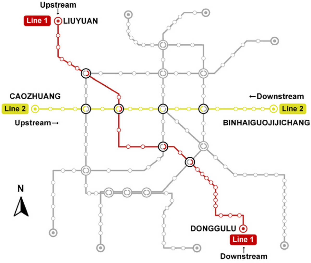
This section employs Tianjin URT Lines 1 and 2 as case studies to validate the effectiveness of the proposed clustering algorithm. Lines 1 and 2 serve as the primary north–south and east–west corridors of the Tianjin URT network, respectively, and constitute essential components of the city’s daily commuting system, as illustrated in Figure 2.

On a typical working day, the average passenger flow on both lines exhibits regular temporal fluctuations, which display a clear bimodal distribution, as illustrated in Figure 3. The current division of operational periods is summarized in

Table 1. Current division of operating periods for Tianjin URT Lines 1 and 2.

Periods	Line 1		Line 2
	Upstream	Downstream	Upstream	Downstream
Morning off-peak	06:00–06:30	06:00–06:30	06:00–06:30	06:00–06:30
Morning peak	06:30–09:00	06:30–09:00	06:30–09:00	06:30–09:00
Midday off-peak	09:00–16:30	09:00–16:30	09:00–16:30	09:00–16:30
Evening peak	16:30–19:00	16:30–19:00	16:30–19:00	16:30–19:00
Evening off-peak	19:00–23:54	19:00–23:41	19:00–23:38	19:00–23:39

.

As shown in Table 1, the existing time divisions for Lines 1 and 2 are generally consistent, with the only difference being the end time of the late off-peak period, which is caused by variations in last train operation times. The division of operational periods for the upstream and downstream directions of the same line also demonstrates a certain degree of temporal symmetry. However, Figure 3 reveals that the passenger flow characteristics of the two lines differ, a discrepancy that is not reflected in the current period division schemes.

To ensure consistency in the temporal scope of all samples, the operational period for both directions of Lines 1 and 2 is standardized to 06:00–23:59. Based on Equation (11), the sample space $S$ is constructed accordingly, consisting of 1079 samples and 9 features.

All algorithms in this study were implemented in MATLAB 2021b and executed on a personal computer equipped with an Intel i7-14700HX CPU (Intel Corporation, Santa Clara, CA, USA) and 16 GB of RAM (Ramaxel Co., Ltd., Shenzhen, China), and the Windows 11 operating system. Prior to the clustering analysis, the sample data are normalized using min-max standardization.

5.2. Clustering Results and Discussion

This section first presents the preliminary clustering results of the SOM applied to the initial sample space.

5.2.1. SOM Topology Size

A two-dimensional SOM network of size $n\times n$ is employed to perform preliminary clustering on the original samples, where $n$ denotes the number of neurons along each dimension. The topology size directly affects the network’s ability to represent the input space with sufficient granularity, as well as the computational efficiency. An undersized SOM may fail to capture the intrinsic structure of the data, leading to reduced clustering performance, whereas an oversized topology may result in redundant representations and increased training time.

To evaluate the impact of different SOM network sizes ($n\times n$) on overall clustering performance, a performance metric $I_n$ is designed to simultaneously reflect clustering accuracy and training efficiency under varying topological scales, as expressed in Equation (22).

$$I_n=J_n+T_n$$

(22)

Here, $J_n$ denotes the sum of the distance between each sample and the weight vector of its corresponding neuron in the clustering results obtained from the SOM network of size $n$, as defined in Equation (23). $T_n$ represents the training time (in seconds) of the SOM network with topology size $n$.

$$J_n={\displaystyle \sum _{i=1}^{N-1}‖x_i-W_{(x_i)}^{*}‖}$$

(23)

where $W_{(x_i)}^{*}$ denotes the weight vector of the neuron corresponding to sample $x_i$ after SOM training. To eliminate dimensional differences, both $J_n$ and $T_n$ were standardized prior to calculating $I_n$. A smaller value of the performance metric $I_n$ indicates better overall clustering performance.

Figure 4 illustrates the variation in $I_n$ with the SOM topology size $n$ across different lines. In each scenario, the network was trained independently 20 times with an initial learning rate of ${\eta }_0=0.8$ and 1000 training iterations, and the average value of $I_n$ was reported. The parameter $n$ was varied from 3 to 32. Based on the results, the optimal SOM network structures were determined to be 14 × 14 for Line 1 (both directions) and Line 2 (upstream), and 12 × 12 for Line 2 (downstream).

5.2.2. Parameter Sensitivity Analysis

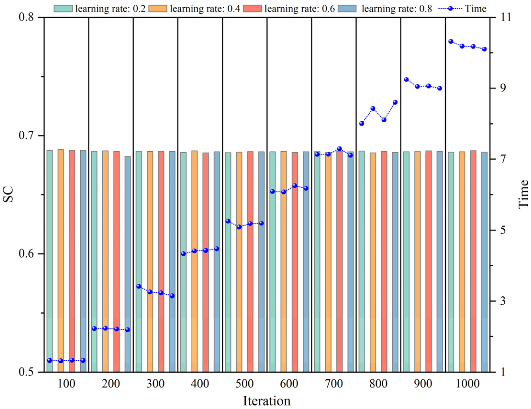
To systematically evaluate the sensitivity of the SOM model to parameter settings, the upstream direction of Line 1 was selected as a case study. Two parameters were examined: the number of iterations and the initial learning rate. These parameters play distinct roles in SOM training: the former primarily determines the convergence of network weights, while the latter affects both the convergence speed and the adequacy of training. Multiple parameter combinations were designed, and the resulting silhouette coefficients and computation times were compared to assess the stability and computational cost of SOM under different configurations, as illustrated in Figure 5.

As shown in Figure 5, the silhouette coefficient remained nearly constant across different parameter combinations, with only negligible fluctuations. This indicates that the clustering boundaries and intra-cluster compactness of SOM–K-means are largely unaffected by parameter variations. Specifically, increasing the number of iterations did not yield further improvements in clustering performance, suggesting that the algorithm achieves convergence rapidly. Similarly, while different initial learning rates influenced the rate of weight updates during training, the final clustering results were consistent. These findings demonstrate the robustness of SOM–K-means in operating period division, with clustering performance insensitive to parameter perturbations.

In contrast, the computational efficiency exhibited clear dependency on parameter settings. For a fixed number of iterations, varying the initial learning rate had almost no effect on runtime, indicating that the step size of updates contributes little to the overall computational complexity. However, increasing the number of iterations substantially prolonged computation time in an approximately linear manner. This trend is consistent with the iterative mechanism of SOM, where each additional iteration requires a full traversal of the samples and weight updates, resulting in computation time proportional to the number of iterations.

In summary, SOM–K-means exhibited stable clustering performance across a wide range of parameter values, with neither the number of iterations nor the initial learning rate significantly affecting clustering validity. Nevertheless, runtime was highly sensitive to the number of iterations, where excessive iterations markedly increased the computational burden without performance gains. Considering this trade-off, the parameter combination of 100 iterations and an initial learning rate of 0.4 was selected in this study, achieving a balance between accuracy and efficiency while avoiding unnecessary computational redundancy.

5.2.3. Pre-Clustering Results by SOM

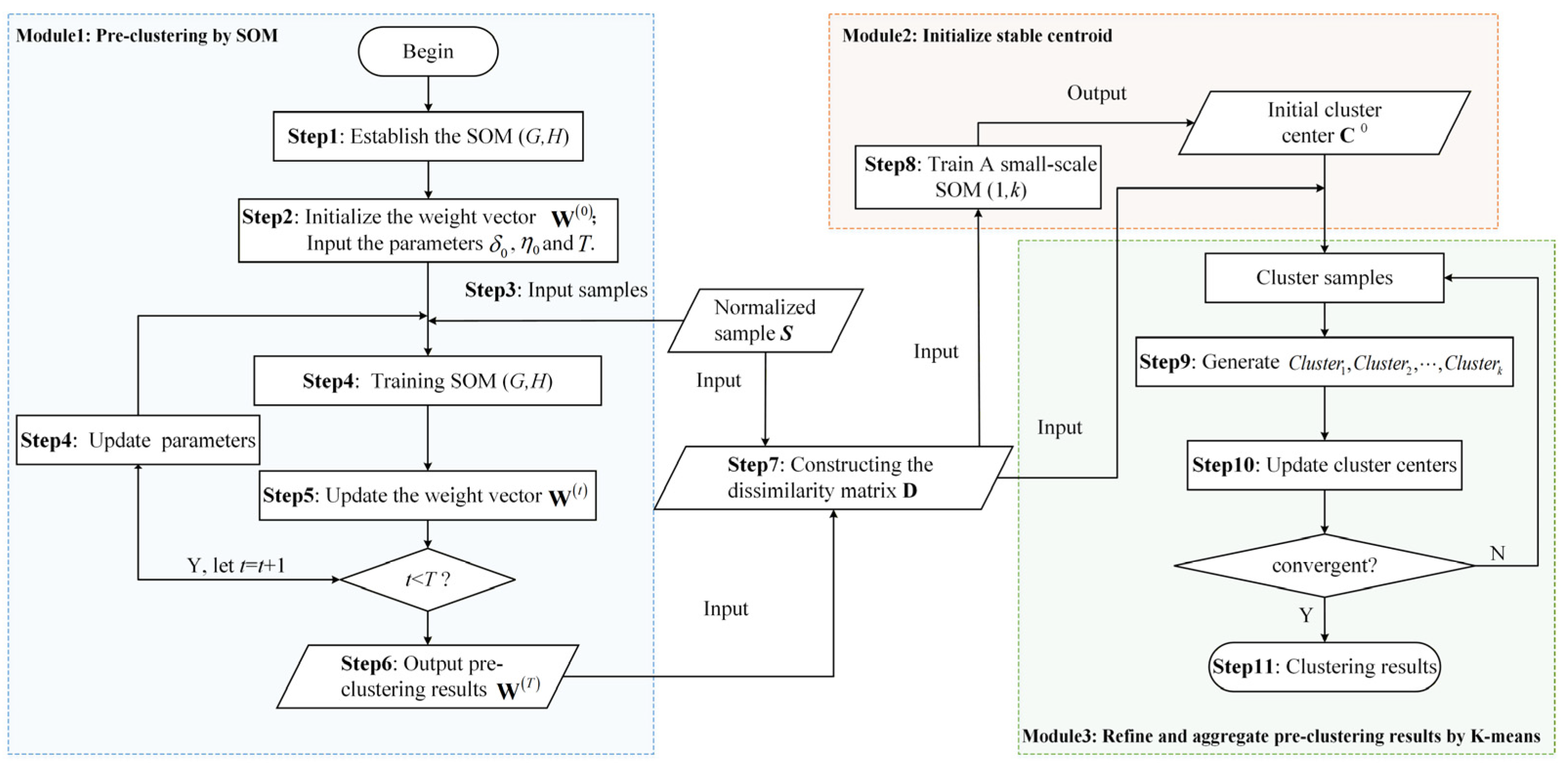
Based on the SOM–K-means algorithm proposed in Section 4, this subsection first applies the SOM component to perform pre-clustering on the raw data. The core advantage of SOM lies in its topology-preserving property—it can map high-dimensional passenger flow features onto a low-dimensional (two-dimensional) neuron grid while retaining the similarity structure of the original data [39]. 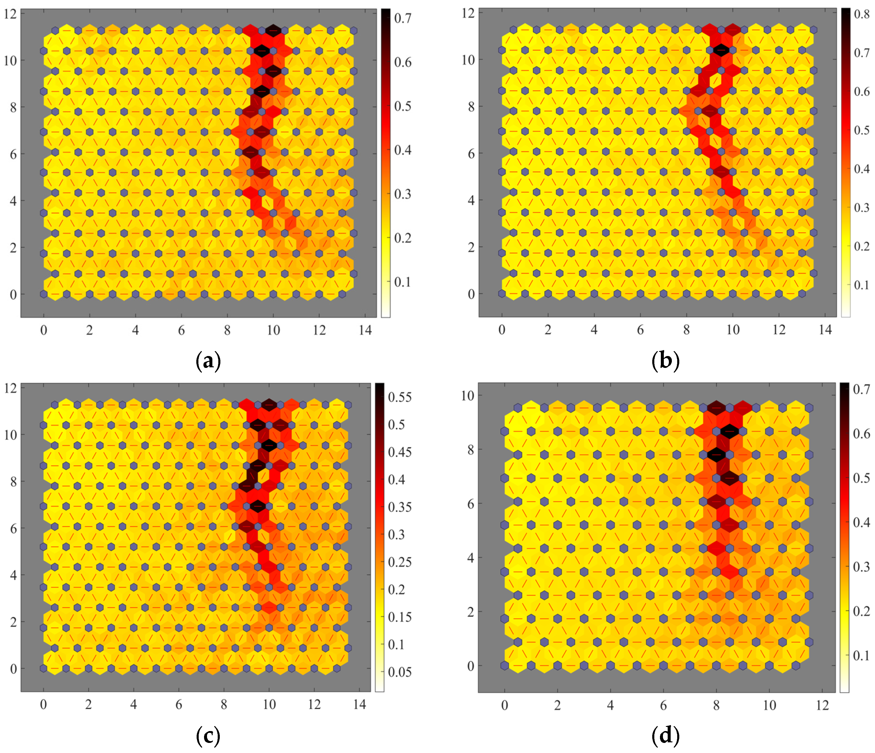Meanwhile, SOM provides a visualization technique for multidimensional clustering results, enabling an intuitive understanding of the relationships among data [40]. Through SOM pre-clustering, data samples with similar passenger flow patterns are merged into adjacent neurons, whereas those with distinct patterns are assigned to neurons with larger distances. The U-matrix is then used to visualize the topological relationships among neurons.

Figure 6 illustrates the preliminary clustering results using the U-matrix. The U-matrix depicts the distance distribution between neighboring neurons after SOM training. In the figure, light-colored regions indicate small differences between adjacent neurons, reflecting similar passenger flow patterns, whereas dark-colored regions correspond to larger differences, representing potential cluster boundaries.

Across all four directions, the U-matrix visualization reveals a prominent dark boundary that divides the map. Overall, the left side of the map exhibits large, contiguous light-colored regions, indicating high feature homogeneity among the corresponding time periods. Considering the actual URT operation, this region corresponds to off-peak periods characterized by stable and low-variation passenger demand. In contrast, the right side of the boundary contains several smaller light-colored regions, representing relatively consistent patterns of limited scope, which correspond to typical peak-hour periods. The dark nodes between these regions indicate blurred cluster boundaries, reflecting the complexity of passenger flow dynamics, such as the ramp-up and ramp-down phases of morning and evening peaks. Notably, isolated dark nodes are also observed in boundary regions, likely corresponding to time periods with abnormal characteristics, such as the start of service or late-night low-demand intervals.

Overall, the U-matrix visualization demonstrates that the SOM effectively captures the main structures of passenger flow patterns, while also highlighting issues of overly fine clustering and ambiguous boundaries. From an operational perspective, directly adopting the preliminary clustering results could lead to an excessively fragmented timetable, which presents several challenges. First, too many time intervals would cause frequent changes in train headways, increasing vehicle circulation complexity and the risk of operational delays. Second, crew scheduling would become more difficult, further complicating dispatching tasks. These factors could ultimately reduce the reliability and robustness of the timetable, adversely affecting passenger service quality. Furthermore, due to the inherent topological constraints of SOM, relationships between non-adjacent neurons cannot be effectively captured. Therefore, in practice, it is necessary to further integrate and refine the preliminary clustering results to develop a more concise and robust operating period scheme, thereby ensuring operational feasibility in practice. This is the core reason for the subsequent introduction of K-means in this study.

5.2.4. Clustering Results Refined by K-Means

To address the limitations of SOM pre-clustering, K-means clustering is introduced in this section to overcome the local topological constraints of SOM. From a global perspective, it merges feature-similar pre-clustering results and generates an operational period division scheme that supports practical operational decision-making.

First, a dissimilarity matrix $D_{1079\times 169}$ is constructed based on the weight vectors of all neurons in the trained SOM network and the original sample data. Each element in the matrix represents the Euclidean distance between a sample and a neuron, effectively projecting the original high-dimensional data into a distance space defined by the neurons. In the process of operational time-period division, compared with directly measuring sample similarity based on “sample-to-sample distance”, the “sample-to-neuron distance” not only preserves the inherent structural differences among original samples but also smooths data noise, reducing the impact of outliers on the clustering results. As previously mentioned in Section 4.1, the dissimilarity matrix $D$ is used as the input for K-means and captures the similarity between samples by measuring their relative distances to all neurons.

The high dimensionality of the dissimilarity matrix $D$ makes K-means highly sensitive to the initialization of cluster centers. Randomly selecting $k$ samples from $D$ as the initial cluster centers may cause the algorithm to fall into a local optimum, thereby directly lead to instability and reduced clustering accuracy. To address this issue, a SOM network with a topology of $\left(1,k\right)$ is constructed to generate initial cluster centers. The training parameters of this SOM are consistent with those used for the pre-clustering SOM, except that the number of training iterations is reduced to 20 to improve the efficiency of cluster centers initialization.

Theoretically, after a small number of training iterations, this small-scale SOM exhibits a certain degree of distance and distinction among its $k$ weight vectors. Using these weight vectors as the initial centroids for K-means enables the centroids to be evenly distributed across different passenger flow pattern groups, thereby preventing the initial centroids from being too close to each other, accelerating the convergence of the algorithm toward the global optimum, and improving clustering stability.

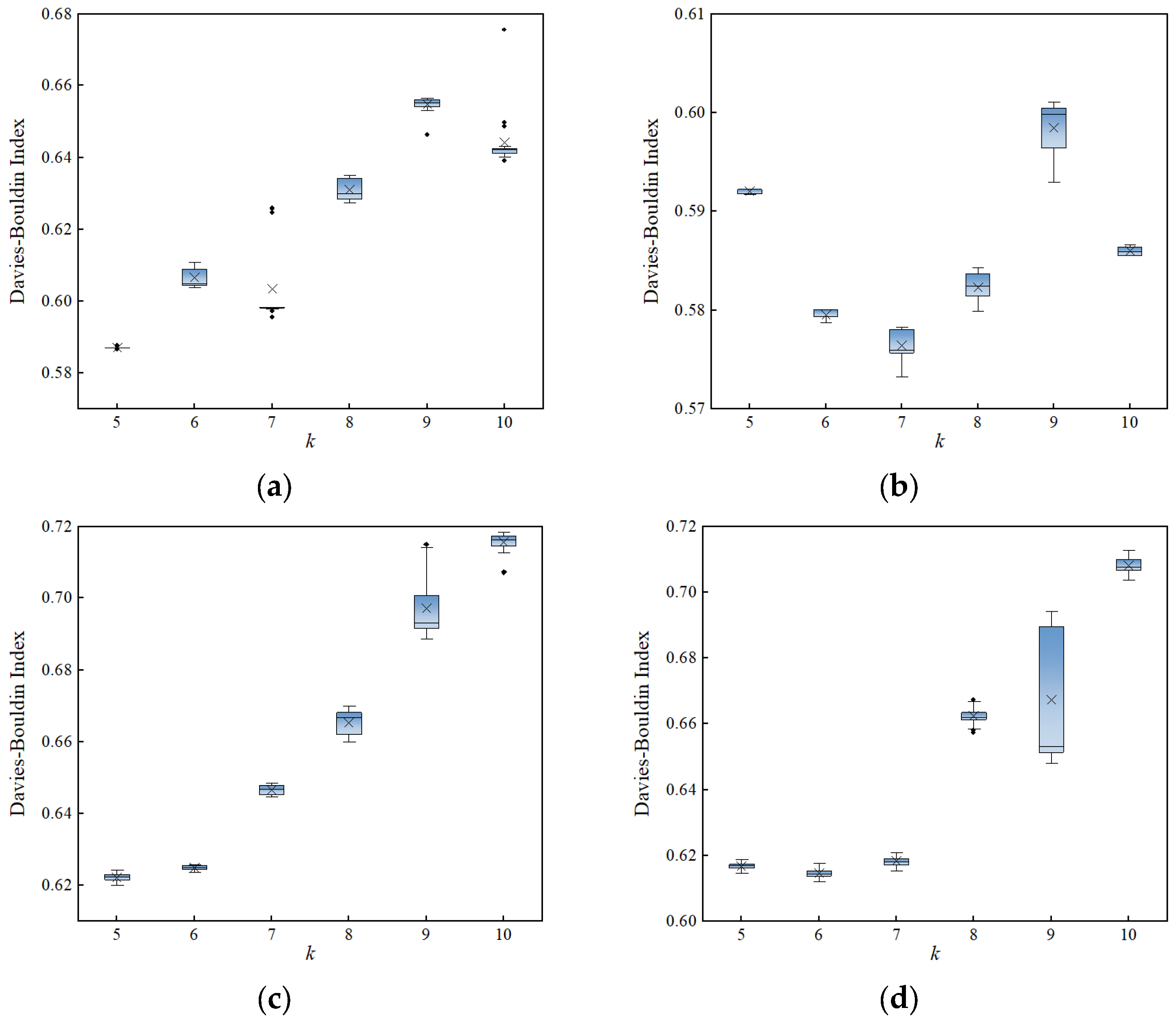
The value of $k$ is set from 5 to 10 with an increment of 1. The improved K-means is then applied to cluster the dissimilarity matrix $D$. For each value of $k$, the algorithm is independently executed 20 times. The DBI values are calculated according to Equation (19) and illustrated in Figure 7.

As shown in Figure 7, applying K-means clustering with initial centers generated by the SOM network yields more stable clustering results, particularly for the upstream direction of Line 2. For each set of repeated experiments, the maximum variation in the DBI does not exceed 0.05, with the largest fluctuation observed in the downstream direction of Line 2 (at $k=9$). According to the definition of DBI, relatively low DBI values indicate that clusters are well separated and internally consistent, which means that the passenger demand patterns represented by samples in different periods have clearer boundaries. The train scheduling plan formulated based on the clustering-derived period schemes can more accurately match the passenger demand patterns of each cluster. Conversely, high DBI values indicate insufficient distinction between clusters, and some operating periods may simultaneously contain multiple different passenger demand patterns. This mixed characteristic makes it difficult to develop targeted train operation plans, reducing the precision with which train scheduling meets passenger demand. The DBI analysis shows that the optimal number of clusters for the four directions shown in Figure 7 is determined to be 5, 7, 5, and 6, respectively.

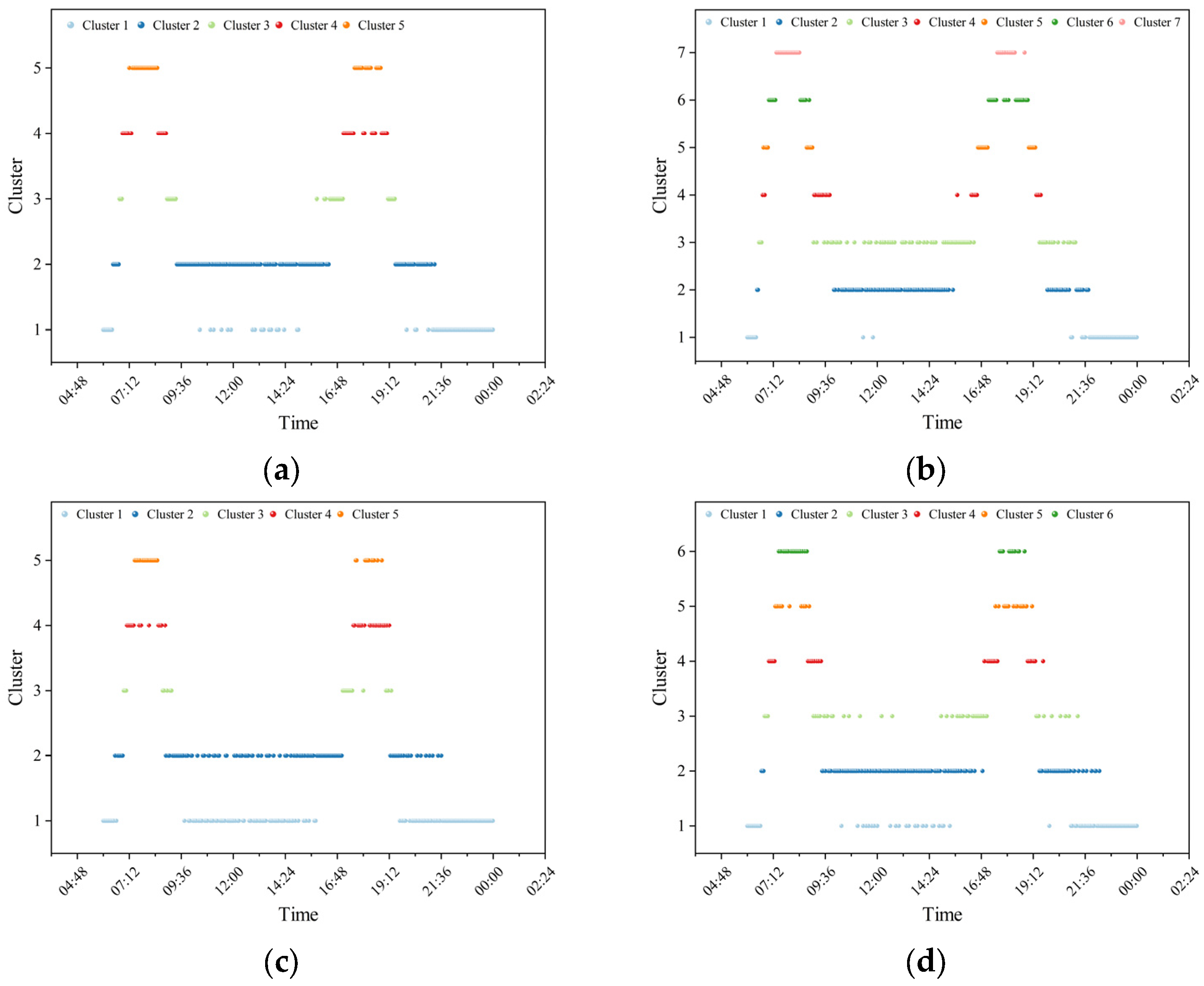
Figure 8 illustrates the clustering-based division of operating periods across different lines. Unlike previous studies [8,9,16], this paper constructs clustering samples at a 1 min resolution, which significantly improves the accuracy of the period division scheme. Overall, the clustering results clearly show the various operational stages throughout the full-service day. Although the number of clusters differs across lines, the outcomes consistently capture temporal variations in passenger demand. However, such fine granularity also leads to the occurrence of isolated points in the clustering results. Therefore, further refinement and integration of the clustering outcomes is necessary.

Taking Figure 8a as an example, Cluster 1 represents both the initial start-up stage of daily service and the closing stage near the end of operations, during which passenger volumes are the lowest of the day but exhibit relatively rapid fluctuations. Cluster 2 corresponds to the longest off-peak periods—including the morning, midday, and evening off-peaks—characterized by relatively low and stable passenger volumes, thereby differentiating them from the samples in Cluster 1. Notably, samples belonging to Cluster 1 also appear between 09:30 and 14:30, which can be regarded as outliers relative to Cluster 2.

Clusters 3 and 4 represent transitional stages between off-peak and peak periods, where passenger flows rise rapidly but to varying levels. A clear asymmetry is observed between morning and evening peaks: while the morning peak and its adjacent transitional periods exhibit distinct boundaries, the evening peak shows less pronounced separation. This feature is also evident in Figure 8b. By comparing with the passenger flow patterns shown in Figure 3, it can be observed that the morning peak on weekdays is highly concentrated due to the strong temporal regularity of commuting and schooling activities, whereas the evening peak displays a multi-modal pattern, with some time samples exhibiting characteristics of transitional periods. Although Line 2 exhibits weaker commuting attributes than Line 1, it demonstrates a similar pattern.

The analysis indicates that the introduction of K-means clustering can effectively integrate the SOM pre-clustering results, enabling samples to be accurately distinguished and transforming the pre-clustering outcomes into operationally feasible and interpretable time period divisions. The clustering results effectively capture both the macroscopic and microscopic characteristics of passenger flows, thereby accurately identifying the comprehensive passenger demand reflected by each sample.

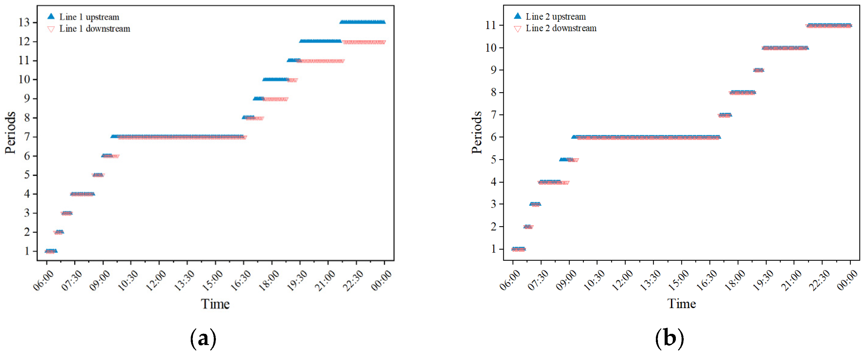
Based on the distinct boundaries revealed by the clustering results, the full-day operating hours can be directly delineated. In this paper, isolated points and time slices with durations of less than 20 min are processed as follows: if the adjacent time samples before and after belong to the same cluster, the slice is merged into that period; otherwise, it is assigned to the subsequent period. Figure 9 illustrates the resulting division of operating periods for different URT lines. As shown in Figure 9a, the upstream direction of Line 1is divided into 13 operating periods. Compared with the existing scheme, the proposed segmentation further refines the major intervals—morning peak (06:30–09:00), midday off-peak (09:00–16:30), evening peak (16:30–19:00), and late off-peak (19:00–23:59)—capturing subtle variations in passenger flow patterns within each period. The downstream direction is divided into 12 periods, also reflecting diverse passenger flow characteristics. In the case of Line 2, although both upstream and downstream directions are divided into 11 operating periods, there are noticeable differences in the temporal coverage of each period, as shown in Figure 9b. Overall, the newly defined operating periods for both lines exhibit clear asymmetry between directions, which contrasts with the previously established symmetric structure.

In summary, this study achieves a precise division of urban rail transit operation periods through a two-stage approach of “SOM pre-clustering—K-means cluster refinement.” The SOM, leveraging its strengths in high-dimensional data processing, performs noise smoothing and dimensionality reduction visualization on the original multi-dimensional passenger flow data, and constructs a dissimilarity matrix based on weight vectors, thereby providing a structural foundation for accurate period segmentation. However, the pre-clustering results of SOM are constrained by local topological structures, which may lead to cluster fragmentation. To address this, K-means utilizes the initialization centroids provided by the small-scale SOM to stably aggregate the pre-clustering results into an operation period division scheme that balances feature accuracy and operational feasibility. In Section 5.3, the SOM–K-means method is compared with other clustering algorithms in terms of clustering performance and stability, further highlighting the applicability and effectiveness of this hybrid clustering framework in the division of urban rail transit operation periods.

5.2.5. Asymmetry in the Operating Periods

Based on the clustering results presented in this study, the initially derived division scheme can be further adjusted to enhance its applicability in practice.

Table 2. Comparison of Line 1 operating periods before and after clustering.

Periods	Upstream		Downstream
	Current	Cluster	Current	Cluster
Morning off-peak	06:00–06:30	06:00–07:00	06:00–06:30	06:00–06:30
Transition period	—	07:00–07:30		06:30–07:00
Morning peak	06:30–09:00	07:30–09:00	06:30–09:00	07:00–09:00
Transition period	—	09:00–09:30		09:00–09:30
Midday off-peak	09:00–16:30	09:30–16:30	09:00–16:30	09:30–17:00
Transition period	—	16:30–17:00		17:00–17:30
Evening peak	16:30–19:00	17:00–19:00	16:30–19:00	17:30–19:00
Transition period	—	19:00–19:30		19:00–19:30
Evening off-peak	19:00–23:54	19:30–21:40	19:00–23:41	19:30–21:50
Late-night period	—	21:40–23:59		21:50–23:59

Note: All time intervals are defined as inclusive of the start time and exclusive of the end time.

and

Table 3. Comparison of Line 2 operating periods before and after clustering.

Periods	Upstream		Downstream
	Current	Cluster	Current	Cluster
Morning off-peak	06:00–06:30	06:00–07:00	06:00–06:30	06:00–06:30
Transition period		07:00–07:30		06:30–07:00
Morning peak	06:30–09:00	07:30–08:30	06:30–09:00	07:00–09:00
Transition period		08:30–09:00		09:00–09:30
Midday off-peak	09:00–16:30	09:00–17:00	09:00–16:30	09:30–17:00
Transition period		17:00–17:30		17:00–17:30
Evening peak	16:30–19:00	17:30–19:00	16:30–19:00	17:30–19:00
Transition period		19:00–19:30		19:00–19:30
Evening off-peak	19:00–23:38	19:30–21:50	19:00–23:39	19:30–21:40
Late-night period		21:50–23:59		21:40–23:59

Note: All time intervals are defined as inclusive of the start time and exclusive of the end time.

show a comparison of the adjusted division schemes for each line direction with the original scheme.

Compared with the original scheme, the adjusted operating periods exhibit pronounced asymmetry, both across different lines and between opposite directions of the same line. Specifically, on Line 1, the morning peak in the upstream direction begins 30 min later than the downstream direction, though both end at 09:00. During the evening peak, the upstream direction starts earlier by 30 min, while both directions conclude simultaneously at 19:00. On Line 2, differences between directions are mainly observed during the morning peak, with the upstream period from 07:30 to 08:30 and the downstream period from 07:00 to 09:00, lasting twice as long as the upstream period.

The observed asymmetry in operating periods arises from the uneven distribution of passenger flows, highlighting the necessity of analyzing operating period divisions based on actual passenger flow patterns.

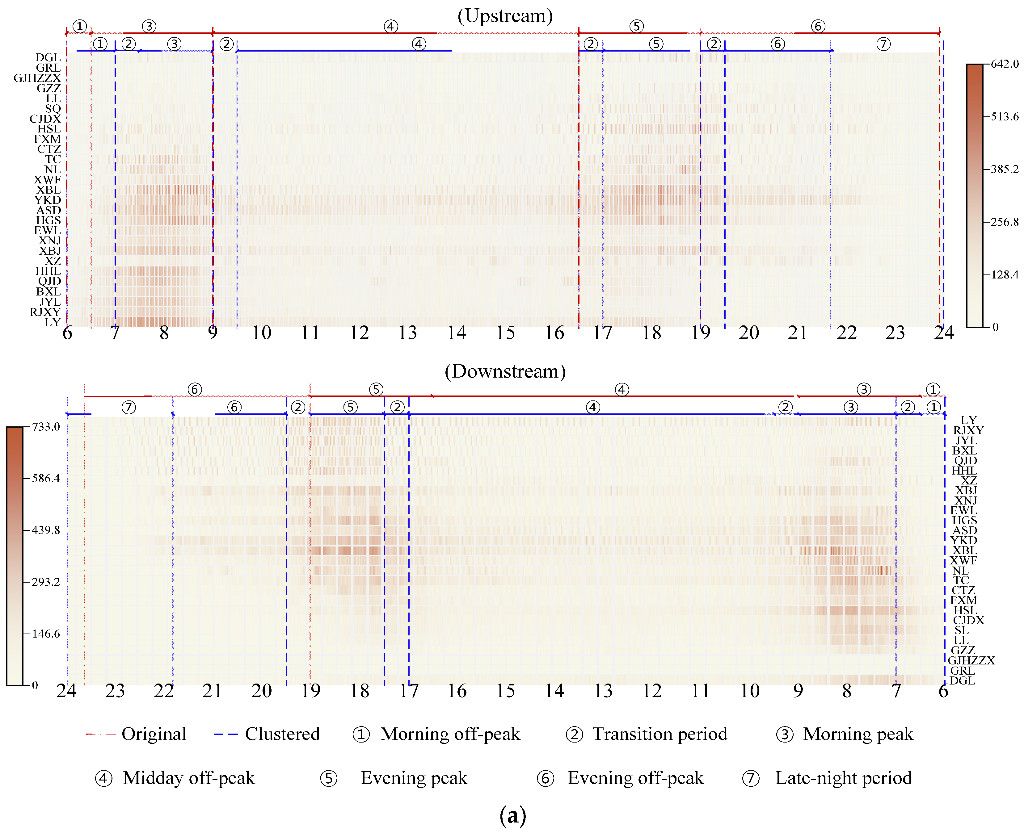
Figure 10 intuitively illustrates the relationship between the divided operating periods and the spatiotemporal distribution of passenger flow by overlaying the division results of each line on the corresponding passenger flow heatmap. The passenger flow at each station and time interval represents the total number of entries and exits over five consecutive working days. Overall, passenger flow on all lines exhibits a typical bimodal pattern. However, significant differences in flow intensity are observed within the same times, and the peak-hour demand centers differ between the two directions. For instance, Line 1 displays a distinct tidal pattern during both morning and evening peaks, with peak demand occurring at different times for each direction. In contrast, Line 2 shows greater asymmetry in passenger flow patterns. During the morning peak, the upstream direction experiences a more concentrated demand, with peak passenger volume lasting only one hour, yet the total flow is noticeably higher than that of the downstream direction. This directional asymmetry highlights the need for differentiated operating period divisions.

The clustering-based period boundaries (blue dashed line) align closely with these observed variations. Taking Line 1 as an example, the morning off-peak in the up direction is extended to 06:00–07:00, corresponding to the relatively low passenger volume during this time. Subsequently, the period from 07:01 to 07:30 serves as a transition period, during which passenger flow rapidly increases from a low to a high level. The morning peak period (07:31–9:00) maintains a consistently high passenger volume, followed by a transition stage (09:01–9:30) when passenger demand gradually declines. The subsequent off-peak period (09:31–16:30) remains stable at a low level. From 16:30 to 17:00, the system enters a transition from midday off-peak to the evening peak, during which passenger flow rises sharply. The evening peak (17:01–19:00) lasts for two hours, showing a high-level passenger volume, followed by a short decline between 19:01 and 19:30. Then came the evening off-peak period (19:31–21:40), with passenger flow levels similar to the midday off-peak period, maintaining a low and stable level. During the late-night period, passenger demand further decreases until it approaches zero.

In contrast, the morning off-peak period in the down direction lasts only 30 min (06:00–06:30), after which passenger volume increases rapidly. The subsequent transition stage (06:31–7:00) also lasts for half an hour, leading to the morning peak occurring approximately 30 min earlier than in the up direction, lasting for two hours (07:01–9:00). During the evening, the peak in the downward direction (17:31–19:00) is delayed by about 30 min compared with the upward direction (17:01–19:00), indicating that high-density passenger flows are more concentrated in the later period. After the short transition phase (19:01–19:30), passenger demand gradually decreases to a low level, marking the start of the evening off-peak. The down-direction evening off-peak is about 10 min longer than that of the up direction, suggesting that late-night passenger patterns are relatively consistent between the two directions.

Overall, the differences in clustering results between the two directions are mainly concentrated in the morning and evening peaks. The up direction exhibits a more concentrated morning travel pattern, resulting in a shorter peak duration, while the down direction demonstrates a more concentrated evening travel demand. In contrast, the original symmetric scheme (red dashed line) adopts identical operation period divisions in both directions, with morning and evening peaks each lasting 2.5 h (06:31–09:00 and 16:30–19:00), thereby failing to accurately reflect the differences in passenger flow.

These results demonstrate that the proposed clustering-based asymmetric division effectively captures inter-period variations in passenger demand while maintaining strong internal consistency within each period. It further offers valuable implications for operational planning. Specifically, the train departure frequency and the number of operating trains can be flexibly adjusted according to the directional distribution of passenger demand, thereby achieving a precise match between service capacity and travel demand and enhancing the utilization efficiency of transport resources. Furthermore, during periods of significant passenger flow fluctuations (such as transition periods and late at night), train departure intervals can be dynamically adjusted to further optimize capacity allocation and increase train load factors. Overall, this demand-based train operation organization strategy helps promote the refinement and efficiency of urban rail transit operation management and provides a useful reference for building an intelligent dispatching system.

5.3. Evaluation of Clustering Performance and Stability

As previously mentioned, this study adopts the Silhouette Coefficient (SC) as the primary clustering quality metric to evaluate the effectiveness and stability of the proposed method. The SC measures the aggregation of samples within the same cluster and their separation from samples in other clusters, thereby capturing both intra-cluster compactness and inter-cluster distinctiveness. A higher SC value indicates a tighter and more clearly defined clustering structure, which corresponds to superior clustering performance. Owing to its computational efficiency and strong interpretability, SC has been widely applied in unsupervised learning and clustering validation tasks [41,42,43]. 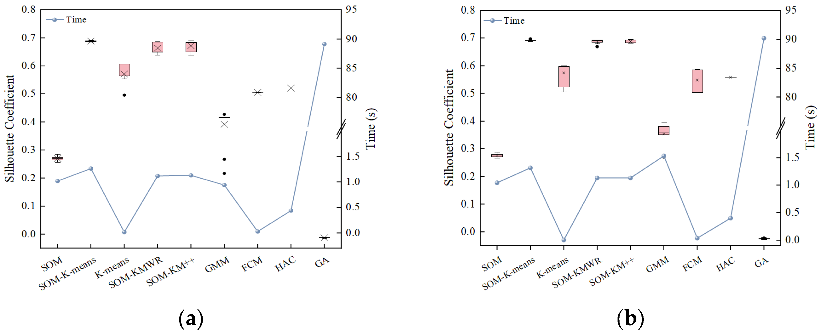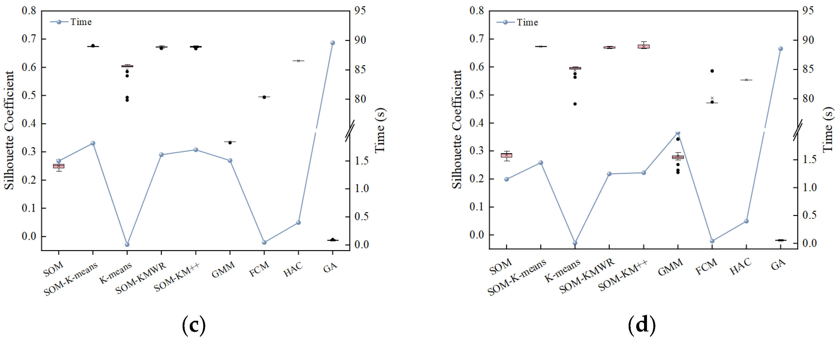Figure 11 illustrates the clustering performance of multiple algorithms, including SOM–K-means, SOM, K-means, SOM–K-means with randomly initialized cluster centers (SOM–KMWR), SOM–K-means++ (SOM–KM++), Gaussian Mixture Model (GMM), Fuzzy C-Means (FCM), Hierarchical Agglomerative Clustering (HAC) and Genetic Algorithm (GA). Each algorithm was independently executed 20 times, with 100 iterations per run. The SC values of the clustering results and the corresponding average computation time were recorded.

As shown in Figure 11, SOM–K-means consistently achieves high SC values across all four URT lines, demonstrating its excellent clustering capability for operational time period segmentation. SOM–KMWR and SOM–KM++ achieve SC values close to those of SOM–K-means, whereas SOM alone exhibits relatively poor performance, and K-means shows moderate performance, falling between the other algorithms. These results indicate that combining SOM with K-means substantially enhances clustering performance.

Table 4. Comparison of the SC values for clustering algorithms across different scenarios.

Algorithm		Line 1 Upstream		Line 1 Downstream		Line 2 Upstream		Line 2 Downstream
		Max SC	Avg SC	Max SC	Avg SC	Max SC	Avg SC	Max SC	Avg SC
SOM–K-means	Value	0.6904	0.6882	0.6966	0.6912	0.6772	0.6745	0.6741	0.6731
	Improvement *	—	—	—	—	—	—	—	—
SOM	Value	0.2696	0.2845	0.2887	0.2760	0.2731	0.2501	0.3004	0.2856
	Improvement	156.08%	142.67%	141.29%	150.43%	147.97%	169.69%	124.40%	136.03%
K-means	Value	0.6073	0.5709	0.6001	0.5745	0.6110	0.5914	0.6001	0.5873
	Improvement	13.68%	20.93%	16.08%	20.31%	10.83%	14.05%	12.33%	14.78%
SOM–KMWR	Value	0.6868	0.6640	0.6931	0.6878	0.6767	0.6720	0.6738	0.6706
	Improvement	0.52%	3.98%	0.50%	0.49%	0.07%	0.37%	0.04%	0.52%
SOM–KM++	Value	0.6893	0.6717	0.6947	0.6879	0.6766	0.6727	0.6909	0.6713
	Improvement	0.16%	2.78%	0.27%	0.48%	0.09%	0.26%	−2.43%	0.42%
GMM	Value	0.4271	0.3918	0.3938	0.3533	0.3364	0.3362	0.3432	0.2815
	Improvement	61.65%	76.21%	76.89%	95.64%	101.31%	100.62%	96.42%	139.47%
FCM	Value	0.5055	0.5055	0.5863	0.5487	0.4950	0.4949	0.5861	0.4888
	Improvement	36.58%	36.58%	18.81%	25.97%	36.81%	36.29%	15.01%	37.91%
HAC	Value	0.5207	0.5207	0.5584	0.5584	0.6235	0.6235	0.5541	0.5541
	Improvement	32.59%	32.59%	24.75%	23.78%	8.61%	8.18%	21.66%	21.66%
GA	Value	−0.0109	−0.0130	−0.0217	−0.0252	−0.0100	−0.0130	−0.0159	−0.0189
	Improvement **	—	—	—	—	—	—	—	—

* Magnitude of improvement achieved by SOM–K-means compared to other clustering algorithms. ** Magnitude of improvement achieved by SOM–K-means is not assessed when the SC value of the comparative algorithm is negative.

further summarizes the mean and maximum SC values for each method, providing a detailed comparison. The quantitative results further corroborate these findings. Across all four scenarios, the mean and maximum SC values produced by SOM–K-means are very close to those of SOM–KMWR and SOM–KM++, with differences within 4%. However, the improvement over other algorithms is considerable, with the vast majority of cases exceeding 10%. Notably, in the downstream direction of Line 2, SOM–KM++ slightly surpasses SOM–K-means in maximum SC value by 2.43%. The GA consistently exhibited the poorest performance across all experimental scenarios, with its maximum SC values remaining negative, indicating that the algorithm was trapped in local optima. According to the definition of SC, a value closer to 1 indicates that each sample is more accurately assigned to its corresponding cluster, suggesting that the passenger flow demand patterns during different periods can be more precisely aligned with their respective time intervals. A scheduling plan developed based on such high-precision clustering can achieve a high degree of correspondence with passenger travel demand, thereby improving system efficiency while ensuring service quality Therefore, to guarantee the specificity and effectiveness of the scheduling strategy, clustering results with higher SC values should be prioritized as the basis for period division. In contrast, clustering results with lower SC values are less likely to yield reasonable operational period segmentation schemes.

Regarding computational time, all algorithms except GA complete 100 iterations within 2 s, with K-means, FCM, and HAC requiring less than 1 s. For the four SOM-based algorithms, runtime is primarily influenced by the number of neurons, showing almost synchronous variation across the four scenarios. GMM, however, exhibits some variability in runtime. GA consumed substantially more computational resources, with runtimes of approximately 90 s in all scenarios, which was markedly higher than those of the other algorithms.

In terms of clustering stability, SOM–K-means, HAC and GA show minimal variation in SC values across 20 independent trials, reflecting their robustness and consistent performance. Due to sensitivity to initial cluster centers, SOM–KMWR and SOM–KM++ still exhibit some stochasticity. This suggests that, with SOM assistance, K-means can effectively mitigate the impact of initialization. By contrast, K-means, GMM, and FCM display larger variability and frequent outliers, reflecting their sensitivity to initialization as well as to the dimensionality and noise inherent in the original samples.

In summary, the SOM–K-means algorithm not only enhances clustering precision but also significantly improves result stability, thereby demonstrating both its effectiveness and adaptability in the context of operating period division for URT.

5.4. Sensitivity Analysis of Clustering Performance and Stability to Sample Size Variations

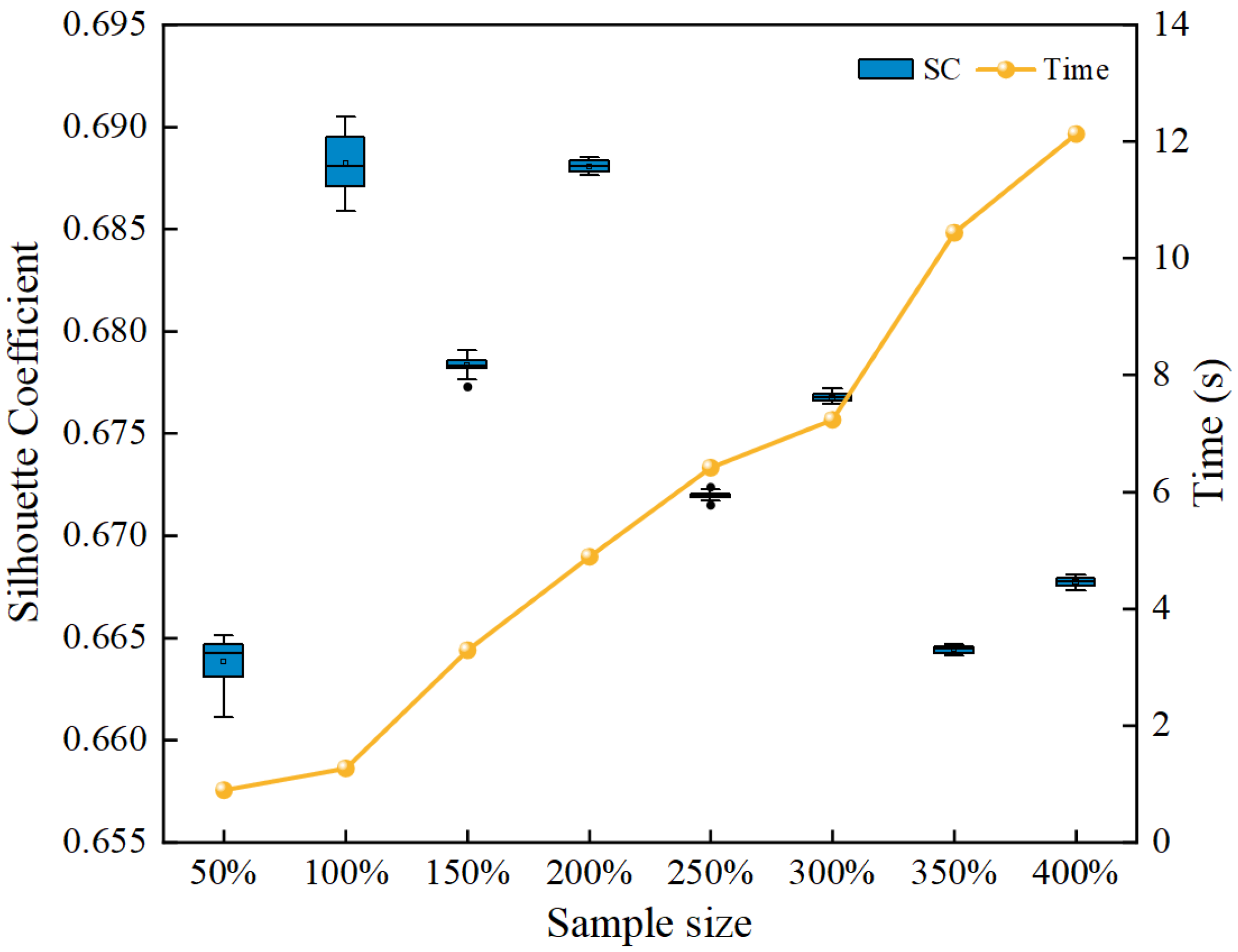
To evaluate the robustness of the proposed SOM–K-means algorithm, experiments were conducted on the upstream direction of Line 1 by varying the sample size to assess the algorithm’s sensitivity to changes in input data volume. The number of neurons was determined using an empirical formula, set as five times the square root of the sample size [26]. For each sample size, the algorithm was independently executed 20 times, and the silhouette coefficient along with the mean computation time were recorded, as shown in Figure 12.

The results indicate that the algorithm achieves consistently high clustering accuracy across different data scales, with only minor fluctuations in silhouette coefficient values (within 0.03), demonstrating robust clustering performance. The slight variations observed over multiple runs further confirm the algorithm’s stability. Additionally, computation time increases approximately linearly with sample size, with the time increment roughly 1.5 times that of the corresponding increase in sample size, indicating low computational complexity and favorable scalability. These findings suggest that SOM–K-means is applicable to clustering datasets of varying sizes.

5.5. Practical Implications

In practical operations, URT operators can utilize the division of operating periods after clustering to re-optimize train headways in line with different operational objectives. Taking the upstream direction of Line 1 as an illustrative example, two alternative headway schemes were simulated to evaluate passenger waiting times and train operations, as summarized in

Table 5. Performance evaluation of different train headway settings.

Periods	Original		Scheme 1		Scheme 2
	Time Span	Headway (min)	Time Span	Headway (min)	Time Span	Headway (min)
Morning off-peak	06:00–06:30	7	06:00–07:00	7	06:00–07:00	7
Transition period	—	—	07:01–07:30	5.5	07:01–07:30	5.5
Morning peak	06:31–09:00	4.4	07:31–09:00	4	07:31–09:00	4.17
Transition period	—	—	09:00–09:30	5.5	09:00–09:30	5.5
Midday off-peak	09:01–16:30	7	09:31–16:30	7	09:31–16:30	7
Transition period	—	—	16:31–17:00	5.5	16:31–17:00	5.5
Evening peak	16:31–19:00	4.4	17:01–19:00	4	17:01–19:00	4.17
Transition period	—	—	19:01–19:30	5.5	19:01–19:30	5.5
Evening off-peak	19:01–22:51	7	19:31–21:40	7	19:31–21:40	7
Late-night period	—	—	21:41–22:40	8	21:41–22:51	8
AWT * (s)	173.94		174.32		178.09
Number of trains	170		170		169

* Average waiting time of passengers.

. Here, “the last time in the period” refers to the departure time of the last train.

In Scheme 1, the original headways are retained during off-peak hours, while train frequency is increased during morning and evening peak periods to better accommodate passenger demand. Transitional periods adopted the mean value between peak and off-peak headways, whereas headways were moderately extended during late-night operations when passenger demand decreases. The results indicate that the average passenger waiting time remained nearly unchanged, with only a slight increase of 0.38 s, while the daily end-of-service time is advanced by 11 min. This earlier termination of service is considered favorable by operators, as it not only reduces operating costs but also facilitates subsequent maintenance activities after service hours.

Scheme 2 builds upon Scheme 1 by slightly extending peak-period headways by approximately 10 s, while keeping all other settings identical. This adjustment results in a modest increase in average passenger waiting time (about 2.16%), but enables the elimination of one train operation, thereby achieving direct cost savings for the operator.

Adjusting train headways based on operational objectives is inherently a train timetable optimization problem [44], which requires balancing passenger demand with operational constraints, such as safety requirements and equipment utilization limits. This study provides decision support for headway adjustments from the perspective of passenger demand. Taking the morning off-peak to peak period as an example: during the early off-peak phase, passenger flow is generally low but increases rapidly; under operational constraints, headways can be moderately extended to make full use of available capacity. In the transitional phase, passenger flow is high and grows quickly, necessitating a gradual reduction in headways to increase train deployment and accommodate the rapidly rising demand. During the peak phase, passenger flow remains high with relatively minor fluctuations, warranting dense and evenly spaced headways to minimize passenger waiting time and enhance operational efficiency.

6. Conclusions

This study develops a data-driven framework integrating Self-Organizing Maps (SOM) and the K-means algorithm for clustering-based division of operating periods in urban rail transit (URT), aiming to overcome the subjectivity and limitations associated with manually predefined time intervals. Clustering samples are constructed from passenger travel data recorded by the AFC system, with feature selection encompassing total volume, microscopic variations, and macroscopic distribution of passenger flow, thereby providing a comprehensive characterization of temporal variations in passenger demand.

Empirical analysis of Lines 1 and 2 of the Tianjin URT demonstrates the effectiveness of the proposed method. The SOM–K-means method demonstrates remarkable overall performance in clustering multi-dimensional time samples driven by passenger flow data. Compared to the existing operating period division scheme, the new scheme effectively identifies transitional phases between off-peak and peak periods and distinguishes the late-night operation period from the evening off-peak hours, thereby producing a more precise division of operating periods. We can apply these results to enhance the efficiency of transportation resource utilization and support fine-grained train scheduling. Moreover, the method successfully captures the uneven distribution of passenger flows across different lines and directions, which is reflected in the pronounced asymmetry observed in the resulting operating period schemes. Accordingly, URT can implement differentiated operational management for different lines. The results demonstrate that data-driven approaches can enhance the rationality and efficiency of operational decision-making in URT, effectively overcoming the limitations of manual methods. In addition, the proposed framework is extensible and can be applied to other transit systems to address similar problems.

This study has potential limitations. Only weekday passenger flows make up the limited scope of the observed data. Special events, such as extreme weather or major public activities, may induce abrupt changes in passenger demand patterns, requiring further validation and adaptation of the proposed method. The selection of clustering features also warrants more profound analysis. Since this study is based solely on a single city and its metro network, the proposed framework may encounter new challenges when applied to other transit systems or cities. For instance, passenger flow data from urban bus systems often lack information on alighting flows. In other cities, the granularity of AFC data in URT may not be consistent with that used in this study, potentially limiting the direct transferability of the model. In addition, the practical applicability of the results is constrained by the availability of the data, preventing a more comprehensive exploration.

Future research will primarily focus on the following aspects: (1) Enhancing the generalizability of the proposed framework by incorporating instance-based transfer learning [45,46], thereby extending its applicability to other cities or transit networks, improving the model’s adaptability to diverse passenger flow patterns, and providing more targeted operating period division schemes. This is a major obstacle to practical implementation. (2) Employing deep learning techniques to achieve end-to-end clustering [47], optimizing the automatic extraction and selection of passenger flow features, and improving the accuracy and reliability of clustering analysis. (3) Integrating optimization techniques to extend the present findings, thereby enabling the design of differentiated strategies for distinct operating periods and improving the efficiency and quality of transit services. (4) Broadening the research scope to explore coordinated operating period division across multiple modes of transportation, with the aim of achieving seamless multi-modal integration.