Global Dynamics and Bifurcation of an Evolutionary Beverton-Holt Model with the Allee Effect

Abstract

We study the global dynamics and bifurcation structure of an evolutionary Beverton–Holt model with Allee effects, a framework that couples ecological constraints with adaptive trait evolution. The model accounts for density dependence, mate limitation, and predator saturation, while traits evolve according to selection gradients that influence reproduction and competition. From an ecological perspective, we show that weak Allee effects create bistability between extinction and survival, while strong Allee effects generate a critical threshold below which populations collapse and above which they persist at carrying capacity. Evolutionary feedback further reshapes these outcomes by shifting thresholds, modifying stability regions, and producing multiple long-term attractors. Biologically, this reveals how demographic pressures such as scarce mates or high predation interact with trait evolution to determine persistence or extinction, and how adaptive responses may rescue populations facing critical density barriers. Our rigorous analysis and simulations demonstrate that eco–evolutionary processes not only alter classical Beverton–Holt outcomes but also provide insight into mechanisms underlying species persistence, extinction risk, and invasion success under Allee constraints.

1. Introduction

Mathematical population models have played a central role in understanding how species interact, persist, or decline under varying ecological pressures. One of the earliest and most enduring models is the discrete Beverton-Holt model [1,2], developed originally for fisheries management. This model captures density-dependent regulation and is widely used in both theoretical and applied population dynamics. For a single species, the model takes the form:

$$x(t+1)={\displaystyle \frac{b}{1+cx\left(t\right)}}x\left(t\right):=r\left(x\left(t\right)\right)x\left(t\right),$$

(1)

where $x\left(t\right)\ge 0$ denotes the population size at time $t\in {\mathbb{Z}}^{+}$, and $b>0$, $c>0$ are parameters representing the intrinsic reproduction rate and intraspecific competition, respectively. The per capita growth rate is given by

$$r\left(x\left(t\right)\right)={\displaystyle \frac{b}{1+cx\left(t\right)}}.$$

As is well established (see, e.g., [3,4,5]), Equation (1) has globally predictable dynamics: if $b\le 1$, the zero equilibrium is globally asymptotically stable; if $b>1$, there exists a unique globally asymptotically stable positive equilibrium:

$$x^{\ast }={\displaystyle \frac{b-1}{c}}.$$

Despite the success of classical ecological models, they often treat traits and fitness as fixed. Beginning in the late 20th century, researchers began to realize the importance of feedback between ecological and evolutionary processes—a realization that gave rise to the field of discrete-time evolutionary population dynamics. Early foundational work by Lande [6,7] applied quantitative genetics to ecological models. Later, Dieckmann and Law, and independently Dercole and Rinaldi [8,9,10], introduced more structured and mechanistic approaches that account for the evolution of continuous traits within populations. However, the most profound conceptual advance came from Vincent and Brown in their seminal book Evolutionary Game Theory, Natural Selection, and Darwinian Dynamics [11]. Their work introduced the now-famous canonical equation of adaptive dynamics, which formalizes how traits evolve in response to selection gradients.

In this study, we build on these advances by incorporating evolutionary trait dynamics into the Beverton-Holt framework. We use discrete-time evolutionary models, since unlike their continuous counterparts, they naturally capture generation-to-generation change, admit rich dynamics including bifurcations and chaos, and reveal multiple attractors and basins of coexistence that are central to understanding evolutionary outcomes. We assume individuals are characterized by a continuous scalar trait v (e.g., size, metabolism, aggressiveness), and that the population evolves around a mean trait u. The trait affects both the growth rate and the competitive interactions among individuals, leading to:

$$b=b(v,u),c=c(v,u).$$

The dynamics of the population size $x\left(t\right)$ and the mean trait $u\left(t\right)$ are then governed by:

$$\begin{array}{cc}\hfill x(t+1)& ={\displaystyle \frac{b(v,u(t\left)\right)}{1+c(v,u(t\left)\right)x\left(t\right)}}{|}_{v=u\left(t\right)}x\left(t\right),\hfill \end{array}$$

(2)

$$\begin{array}{cc}\hfill u(t+1)& =u\left(t\right)+{\sigma }^2{\displaystyle \frac{\partial lnr(x,v,u(t\left)\right)}{\partial v}}{|}_{v=u\left(t\right)},\hfill \end{array}$$

(3)

with

$$r(x,v,u):={\displaystyle \frac{b(v,u)}{1+c(v,u)x}},$$

and ${\sigma }^2>0$ representing the speed of evolution (often proportional to the trait variance). Equation (3) is the canonical equation of adaptive dynamics, and describes how the population mean trait shifts in the direction of the fitness gradient.

For analytical and biological clarity, we assume: $c(v,u)=c(v-u)$ with $c_0=c\left(0\right)$ and $c_1=c^{\prime }\left(0\right)$, $b\left(v\right)=b_0{e}^{-v^2/2}$. Then

$$\begin{array}{cc}\hfill ln\left(r(x,v,u)\right)& =ln\left(b(v,u)\right)-ln\left(1+c(v,u)x\right)\hfill \\ \hfill & =ln\left(b_0\right)-{\displaystyle \frac{v^2}{2}}-ln\left(1+c(v-u)x\right).\hfill \end{array}$$

So that

$${\displaystyle \frac{\partial }{\partial v}}ln\left(r(x,v,u)\right)=-v-{\displaystyle \frac{c^{\prime }(v-u)x}{1+c(v-u)x}}.$$

When $v=u\left(t\right)$ and $x=x\left(t\right)$, this becomes

$$-u\left(t\right)-{\displaystyle \frac{c^{\prime }\left(0\right)x\left(t\right)}{1+c\left(0\right)x\left(t\right)}}=-u\left(t\right)-{\displaystyle \frac{c_{1}x\left(t\right)}{1+c_{0}x\left(t\right)}}.$$

So that

$$\begin{array}{cc}\hfill u(t+1)& =u\left(t\right)+{\sigma }^2\left(-u\left(t\right)-{\displaystyle \frac{c_{1}x\left(t\right)}{1+c_{0}x\left(t\right)}}\right)\hfill \\ & =(1-{\sigma }^2)u\left(t\right)-{\sigma }^2{\displaystyle \frac{c_{1}x\left(t\right)}{1+c_{0}x\left(t\right)}}.\hfill \end{array}$$

Biologically, this framework represents a population where individuals differ by a quantitative trait (size, metabolism, aggressiveness), and selection acts through both intrinsic growth and frequency-dependent competition, yielding eco-evolutionary feedbacks that can drive convergence, branching, or extinction. These interactions are schematically represented in Figure 1, which illustrates how trait-dependent growth, density regulation, and selection gradients are coupled within the Beverton–Holt framework.

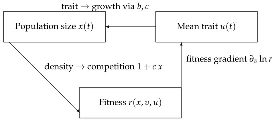
Figure 1. Eco–evolutionary feedback in a discrete-time Beverton–Holt framework. Per-capita growth is $r(x,v,u)={\displaystyle \frac{b(v,u)}{1+c(v,u)x}}$; traits affect b and c, density $x\left(t\right)$ regulates competition, and $u(t+1)=u\left(t\right)+{\sigma }^2{\partial }_{v}lnr(x,v,u){|}_{v=u\left(t\right)}$.

Note that the mean trait may take positive or negative values, with $u=0$ representing the chosen reference baseline. Positive values ($u>0$) correspond to traits above the baseline, while negative values ($u<0$) correspond to traits below it. Figure 2 provides two illustrative cases with opposite sign of the mean trait.

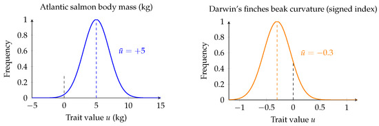
Figure 2. Two examples of species with positive and negative mean trait values. Atlantic salmon mass (left): the blue distribution is centered at $u=+5$ kg. Darwin’s finches beak curvature (right): the orange distribution is centered at $u=-0.3$. Dashed black lines indicate the baseline ($u=0$) and dashed colored lines indicate the mean trait values.

Another vital component of our study is the incorporation of the =Allee effect [3,12,13,14,15,16,17,18,19,20,21,22,23,24]—a phenomenon whereby population growth is suppressed at low densities due to mechanisms such as mate limitation, predator saturation, or cooperative behaviors. The effect was first identified by W. C. Allee in his seminal work [25] and has since been recognized as a critical factor in extinction risk and invasion dynamics. A comprehensive treatment is provided in the book by Courchamp, Berec, and Gascoigne [15], which combines empirical evidence, theoretical models, and case studies to explore the mechanisms generating Allee effects, their consequences for population dynamics, and their implications for both endangered species management and invasive species control. Furthermore, Taylor’s concise encyclopedia entry [26] offers a clear overview of the concept, presenting key definitions, ecological mechanisms, and mathematical models, while highlighting its theoretical and practical relevance in ecological studies.

Allee effects can be classified as:

Definition 1 

([3]). A population model described by the equation $\mathbf{x}(t+1)=F\left(\mathbf{x}\right(t\left)\right)$, with $\mathbf{x}\in {\mathbb{R}}^n,x_i\ge 0\forall i$, is said to exhibit a strong Allee effect if there exists a positive threshold population level such that, when the initial population is below this threshold, the population eventually goes extinct, whereas sufficiently large initial conditions lead to persistence. A weak Allee effect suppresses growth at low densities but does not inevitably lead to extinction.

Mate limitation [27] is a well-studied source of strong Allee effects. To model it, we introduce a fertility term of the form

$${\displaystyle \frac{sx\left(t\right)}{1+sx\left(t\right)}},s>0,$$

which reduces reproductive success when population size is low.

Predator saturation [28] is another important cause of Allee effects: at low prey densities, the per capita predation rate remains high (e.g., due to fixed search behavior of predators), while at higher densities predators become saturated and per capita predation drops. This results in a growth rate that is non-monotonic and may decrease at low density. A standard approach is to model predation pressure as

$$p\left(x\right)=exp\left(-{\displaystyle \frac{m}{1+sx\left(t\right)}}\right),$$

(4)

where the factor

$$exp\left(-{\displaystyle \frac{m}{1+sx\left(t\right)}}\right)$$

represents the effect of the presence of a strong Allee effect due to predator saturation, where m is the attack rate and s is the handling time. We assume that predation mortality increases total competition when x is small. This mechanism can be embedded within the Beverton-Holt form to yield complex nonlinearities.

Bringing all these components together, we propose a general evolutionary Beverton-Holt model incorporating:

• density-dependent growth via the Beverton-Holt mechanism;
• mate limitation via a saturating reproductive term;
• predator saturation as an Allee-inducing mortality factor;
• evolution of a quantitative trait under selection.

For this paper, we simplify the predator saturation mechanism by absorbing it into the net reproductive output and focus on mate limitation explicitly. The resulting coupled system is:

$$\left\{\begin{array}{ccc}\hfill x(t+1)& =& {\displaystyle \frac{b_{0}x\left(t\right)}{1+c_{0}x\left(t\right)}}{\displaystyle \frac{sx\left(t\right)}{1+sx\left(t\right)}}exp\left(-{\displaystyle \frac{u^2\left(t\right)}{2}}\right)\hfill \\ \hfill u(t+1)& =& (1-{\sigma }^2)u\left(t\right)-{\displaystyle \frac{{\sigma }^2{c}_{1}x\left(t\right)}{1+c_{0}x\left(t\right)}}\hfill \end{array},\right.$$

(5)

where, for clarity, we highlight the parameter set

$$b_0>0,s>0,0<c_0<1,c_1\in \mathbb{R},\sigma \in \mathbb{R}.$$

(6)

Notice that the first equation in (5) is the inherent fertility equation while the second equation is the trait equation, more widely known in the literature as the canonical equation for evolution [10], Lande’s equation [6,7] or Fisher’s equation [8]. For comprehensive studies on evolutionary game theory in population dynamics, we refer to the work [18,19,23,24,29,30,31,32,33,34,35].

Objectives of This Study

The goal of this study is to analyze the global dynamics of the evolutionary Beverton-Holt model in Equation (5), which integrates ecological processes (competition, Allee effects from mate limitation and predator saturation) with evolutionary dynamics of traits. Specifically, we aim to:

• Understand how mate limitation and predator saturation induce Allee effects in trait-structured populations;
• Determine the conditions under which the system exhibits multiple attractors, extinction thresholds, and complex dynamics;
• Investigate the influence of evolutionary rates (${\sigma }^2$) on persistence and bifurcation behavior;
• Provide rigorous mathematical analysis and numerical simulations to reveal the long-term outcomes of eco-evolutionary feedbacks in populations subject to Allee effects.

Our study contributes to the growing literature on evolutionary dynamics by highlighting how demographic constraints, such as mate availability and predation pressure, interact with evolutionary change to shape population viability.

2. Fixed Points

System (5) may be viewed as the composition of the mapping $F:({\mathbb{R}}^{+}\times \mathbb{R})\to ({\mathbb{R}}^{+}\times \mathbb{R})$ given by

$$F(x,u)=\left({\displaystyle \frac{b_{0}s{x}^2{e}^{-\frac{u^2}{2}}}{(1+c_{0}x)(1+sx)}},(1-{\sigma }^2)u-{\sigma }^2{\displaystyle \frac{c_{1}x}{1+c_{0}x}}\right).$$

(7)

By a fixed point, we mean a point $(x^{\ast },u^{\ast })$ with $F(x^{\ast },u^{\ast })=(x^{\ast },u^{\ast })$. Clearly, for any parameter values, the origin is a fixed point. We will refer to this as the trivial fixed point of the map (7). For some parameter values, this is the only fixed point. As we will prove momentarily, there can be up to two additional fixed points. Algebraically, these nontrivial fixed points are determined by any $(x,u)$ solution to the system

$$\begin{array}{cc}\hfill {\displaystyle \frac{b_{0}sx{e}^{-\frac{u^2}{2}}}{(1+c_{0}x)(1+sx)}}& =1\hfill \end{array}$$

(8)

$$\begin{array}{cc}\hfill -{\displaystyle \frac{c_{1}x}{1+c_{0}x}}& =u.\hfill \end{array}$$

(9)

Notice that $\sigma$ does not appear in this system of equations. Further, once $c_0$, $c_1$, and s have been specified, there is a critical value $\overline{b_0}$ that determines the number of non-trivial fixed points. Our main theorem on the number of fixed points is the following.

Theorem 1. 

The quartic polynomial

$$c_0^{3}s{x}^4+s(c_1^2+2c_0^2)x^3+(c_1^2-c_0^2+s{c}_0)x^2-2c_{0}x-1$$

(10)

has a unique positive zero $\overline{x}$. Define

$${\overline{b}}_0={\displaystyle \frac{(1+c_0\overline{x})(1+s\overline{x})}{s\overline{x}}}{e}^{{\displaystyle \frac{{\left(c_1\overline{x}\right)}^2}{2{(1+c_0\overline{x})}^2}}}.$$

(11)

Then for any $\sigma \in \mathbb{R}$ the following holds.

1. 

If $b_0<{\overline{b}}_0$, then the only fixed point of mapping (7) is $(0,0)$.

2. 

If $b_0={\overline{b}}_0$, then mapping (7) has two fixed points: $(0,0)$ and $\left(\overline{x},-{\displaystyle \frac{c_1\overline{x}}{1+c_0\overline{x}}}\right)$.

3. 

If $b_0>{\overline{b}}_0$, then mapping (7) has three fixed points: $(0,0)$, $\left(x_A^{\ast },-{\displaystyle \frac{c_1{x}_A^{\ast }}{1+c_0{x}_A^{\ast }}}\right)$, and $\left(x_K^{\ast },-{\displaystyle \frac{c_1{x}_K^{\ast }}{1+c_0{x}_K^{\ast }}}\right)$ where $0<x_A^{\ast }<\overline{x}<x_K^{\ast }$.

Proof. 

We solve the system

$$\begin{array}{cc}\hfill {\displaystyle \frac{b_{0}sx{e}^{-\frac{u^2}{2}}}{(1+c_{0}x)(1+sx)}}& =1\hfill \\ \hfill -{\displaystyle \frac{c_{1}x}{1+c_{0}x}}& =u.\hfill \end{array}$$

by eliminating u, yielding

$${\displaystyle \frac{b_{0}sx{e}^{-\frac{c_1^2{x}^2}{2{(1+c_{0}x)}^2}}}{(1+c_{0}x)(1+sx)}}=1.$$

Let $f\left(x\right)={\displaystyle \frac{b_{0}sx{e}^{-\frac{c_1^2{x}^2}{2{(1+c_{0}x)}^2}}}{(1+c_{0}x)(1+sx)}}-1$, so that any nontrivial fixed point $(x^{\ast },u^{\ast })$ of mapping (7) must satisfy $f\left(x^{\ast }\right)=0$. A calculation shows

$$f^{\prime }\left(x\right)=-{\displaystyle \frac{b_{0}s{e}^{-\frac{c_1^2{x}^2}{2{(1+c_{0}x)}^2}}}{{(1+c_{0}x)}^4{(1+sx)}^2}}\left(c_0^{3}s{x}^4+s(c_1^2+2c_0^2)x^3+(c_1^2-c_0^2+s{c}_0)x^2-2c_{0}x-1\right).$$

Evidently, the sign of $f^{\prime }$ depends only on the quartic

$$c_0^{3}s{x}^4+s(c_1^2+2c_0^2)x^3+(c_1^2-c_0^2+s{c}_0)x^2-2c_{0}x-1.$$

Regardless of the sign of the coefficient $(c_1^2-c_0^2+s{c}_0)$, Descartes’ rule of signs gives that the quartic has exactly one positive root, which we denote $\overline{x}$. Since $f^{\prime }\left(0\right)=b_{0}s>0$, and $f\left(0\right)=-1<0$, f is initially negative and increasing, until it reaches the value $\overline{x}$ where it obtains a maximum. The function f is decreasing afterwards, with $\underset{x\to \infty }{lim}f\left(x\right)=-1<0$. Therefore, the sign of $f\left(\overline{x}\right)$ completely determines the number of positive zeros of f; if $f\left(\overline{x}\right)<0$, then f has no zeros, if $f\left(\overline{x}\right)=0$ then it is the only zero, and if $f\left(\overline{x}\right)>0$ then there are two zeros $x_A^{\ast }$ and $x_K^{\ast }$ with $x_A^{\ast }<\overline{x}<x_K^{\ast }$.

Since $(\overline{x},f\left(\overline{x}\right))$ moves up as $b_0$ increases, there is a unique $b_0$, which we denote ${\overline{b}}_0$, where $f\left(\overline{x}\right)=0$. We can solve $f\left(\overline{x}\right)=0$ algebraically, obtaining

$${\displaystyle \frac{{\overline{b}}_{0}s\overline{x}{e}^{-\frac{c_1^2{\overline{x}}^2}{2{(1+c_0\overline{x})}^2}}}{(1+c_0\overline{x})(1+s\overline{x})}}=1.$$

A rearrangement to solve for ${\overline{b}}_0$ yields the statement of the theorem. □

Remark 1. 

For $b_0>{\overline{b}}_0$, we will refer to $x_A^{\ast }$ as the Allee threshold and $x_K^{\ast }$ as the carrying capacity. One of the main goals of the paper is to describe under what parameter conditions System (5) has a strong Allee effect.

There is also a geometric interpretation of Theorem 1. Consider separately the graphs of

$$\begin{array}{cc}\hfill {\displaystyle \frac{b_{0}sx}{(1+c_{0}x)(1+sx)}}& =e^{{\displaystyle \frac{u^2}{2}}}\hfill \\ \hfill -{\displaystyle \frac{c_{1}x}{1+c_{0}x}}& =u\hfill \end{array}$$

in the $(x,u)$ plane.

If $c_1>0$, $u=-{\displaystyle \frac{c_{1}x}{1+c_{0}x}}$ describes a decreasing convex curve in the fourth quadrant, while if $c_1<0$ it yields an increasing concave curve in the first quadrant. This curve is independent of $b_0$. The first curve is a bit more complicated, and for sufficiently large $b_0$ describes an ellipse-like curve. The size of this graph grows larger as $b_0$ grows. The special value of ${\overline{b}}_0$ is where the two curves are tangent; below this value there is no intersection, and above this value there are two intersections. An example with a numerically computed graphs of these isoclines is given below.

Example 1. 

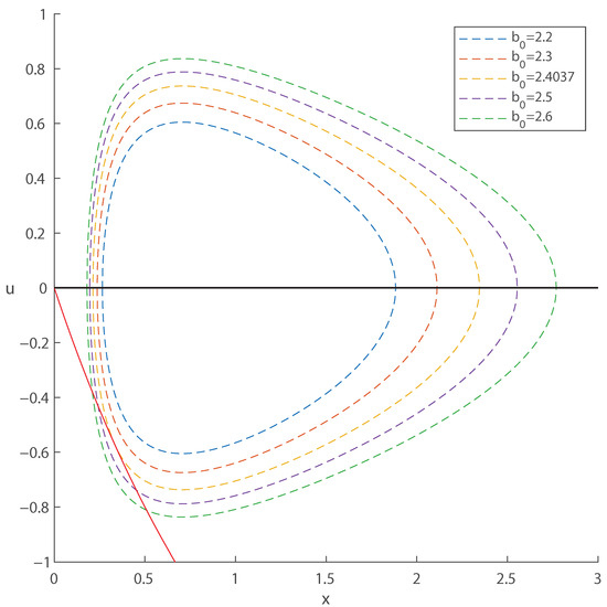
Let $c_0={\displaystyle \frac{1}{2}}$, $s=4$, $c_1=2$. The quartic in Theorem 1 is

$${\displaystyle \frac{1}{2}}{x}^4+18x^3+{\displaystyle \frac{23}{4}}{x}^2-x-1$$

which has a unique positive zero

$$\overline{x}\approx 0.3357.$$

Then, one can substitute that value into

$${\overline{b}}_0={\displaystyle \frac{(1+\frac{1}{2}\overline{x})(1+4\overline{x})}{4\overline{x}}}{e}^{{\displaystyle \frac{2{\overline{x}}^2}{{(1+\frac{1}{2}\overline{x})}^2}}}$$

to obtain ${\overline{b}}_0\approx 2.4037$. A plot at this specific value of ${\overline{b}}_0$, generated using MATLAB 2025a [36], together with neighboring $b_0$ values, is shown in Figure 3.

Figure 3. The relative position of the isoclines determines the non-trivial fixed points. The solid curve represents the isocline $u=-{\displaystyle \frac{c_{1}x}{1+c_{0}x}}$. If there is no intersection, then the origin is the unique fixed point. If there is a single intersection, the system has two fixed points: the origin and an interior fixed point. In the third scenario, when the isoclines intersect at two points, the system admits three fixed points: the origin and two interior fixed points, the Allee threshold and the carrying capacity. The parameter values here are $c_0={\displaystyle \frac{1}{2}}$, $s=4$, $c_1=2$ and $b_0$ as labeled. The diameter of the closed curved increases with $b_0$, with the point of tangency with the line occurring precisely at ${\overline{b}}_0$. This curve is symmetric about the x axis.

In Theorem 1, ${\overline{b}}_0$ is dependent on three parameters. However, it can also be expressed in terms of two parameter ratios, as described in Theorem 2.

Theorem 2. 

The bifurcation value ${\overline{b}}_0$ as defined in Equation (11) can be expressed as a function of the ratios ${\displaystyle \frac{c_1}{c_0}}$ and ${\displaystyle \frac{s}{c_0}}$.

Proof. 

The quartic polynomial may be rewritten as

$${\displaystyle \frac{s}{c_0}}{\left(c_{0}x\right)}^4+{\displaystyle \frac{s}{c_0}}\left({\displaystyle \frac{{c_1}^2}{{c_0}^2}}+2\right){\left(c_{0}x\right)}^3+\left({\displaystyle \frac{{c_1}^2}{{c_0}^2}}-1+{\displaystyle \frac{s}{c_0}}\right){\left(c_{0}x\right)}^2-2\left(c_{0}x\right)-1=0.$$

As a quartic polynomial in $y=c_{0}x$, the coefficients are all functions of ${\displaystyle \frac{c_1}{c_0}}$ and ${\displaystyle \frac{s}{c_0}}$, so that the unique positive root may be expressed as $y^{\ast }=c_0\overline{x}=H\left({\displaystyle \frac{c_1}{c_0}},{\displaystyle \frac{s}{c_0}}\right)$ for some real valued function H.

Then

$$\begin{array}{cc}\hfill {\overline{b}}_0& ={\displaystyle \frac{(1+c_0\overline{x})(1+s\overline{x})}{s\overline{x}}}{e}^{{\displaystyle \frac{{\left(c_1\overline{x}\right)}^2}{2{(1+c_0\overline{x})}^2}}}\hfill \\ & ={\displaystyle \frac{(1+y^{\ast })(1+\frac{s}{c_0}{y}^{\ast })}{\frac{s}{c_0}{y}^{\ast }}}{e}^{{\displaystyle \frac{{\left(\frac{c_1}{c_0}{y}^{\ast }\right)}^2}{2{(1+y^{\ast })}^2}}}\hfill \end{array}$$

and the result follows. □

A plot of the bifurcation point ${\overline{b}}_0$ as a function of $\frac{s}{c_0}$ for different values of $\frac{c_1}{c_0}$, generated using MATLAB 2025a [36], is shown in Figure 4.

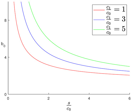
Figure 4. A plot of the bifurcation values ${\overline{b}}_0$ as a function of ${\displaystyle \frac{s}{c_0}}$ for different values of ${\displaystyle \frac{c_1}{c_0}}$. To the lower left of each curve, there is no interior fixed point. An interior fixed point emerges at the bifurcation values, and to the upper right of the curve there are two interior fixed points.

We now describe the curve $e^{{\displaystyle \frac{u^2}{2}}}={\displaystyle \frac{b_{0}sx}{(1+c_{0}x)(1+sx)}}$ more formally, and prove that at ${\overline{b}}_0$ the two curves are tangent. For sufficiently small $b_0$, the curve is empty.

Lemma 1. 

The set of $(x,u)$ that satisfy

$$e^{{\displaystyle \frac{u^2}{2}}}={\displaystyle \frac{b_{0}sx}{(1+c_{0}x)(1+sx)}}$$

is nonempty if and only if

$${\left(\sqrt{{\displaystyle \frac{c_0}{s}}}+1\right)}^2\le b_0.$$

Proof. 

Due to the argument of the exponential, the set is nonempty if and only if

$${\displaystyle \frac{b_{0}sx}{(1+c_{0}x)(1+sx)}}\ge 1.$$

This is equivalent to the quadratic

$$1+(c_0+s-b_{0}s)x+c_{0}s{x}^2\le 0.$$

Since this quadratic is positive at 0 and as $x\to \infty$, it can only obtain negative values if it has two positive real roots. Clearly, if $c_0+s-b_{0}s\ge 0$ this cannot happen, so we assume that the linear term has a negative coefficient. Then since the product of the two roots is ${\displaystyle \frac{1}{c_{0}s}}>0$ and the sum of the two roots is also positive, the set is nonempty if and only if the discriminant of the quadratic is nonnegative.

The discriminant of this quadratic is

$${(c_0+s-b_{0}s)}^2-4c_{0}s=(c_0+s-b_{0}s-2\sqrt{c_{0}s})(c_0+s-b_{0}s+2\sqrt{c_{0}s})$$

and since $c_0+s-b_{0}s<0$ the discriminant is nonnegative if and only if

$$c_0+s-b_{0}s+2\sqrt{c_{0}s}\le 0.$$

This is equivalent to ${(\sqrt{c_0}+\sqrt{s})}^2\le b_{0}s$ or equivalently

$${\left(\sqrt{{\displaystyle \frac{c_0}{s}}}+1\right)}^2\le b_0.$$

Note that this inequality also implies the earlier assumed condition of

$$c_0+s-b_{0}s<0.$$

□

Now we consider $b_0$ so that the set is nonempty. When ${\left(\sqrt{{\displaystyle \frac{c_0}{s}}}+1\right)}^2<b_0$ the isocline describes a closed and mirrored curve $\gamma$ which crosses the u axis at the zeros $0<r_1<r_2$ of

$$1+(c_0+s-b_{0}s)x+c_{0}s{x}^2.$$

It reaches its maximum in the first quadrant at $x=x_M={\displaystyle \frac{-(c_0+s-b_{0}s)}{2c_{0}s}}$ and respectively its minimum in the fourth quadrant at the same value. It represents an increasing curve for positive u on $[r_1,x_M]$ and a decreasing curve thereafter. This is mirrored for negative u, yielding an ellipse-like figure for $\gamma$.

Theorem 3. 

Let ${\overline{b}}_0$ be described as in Theorem 1. Then the curves $e^{{\displaystyle \frac{u^2}{2}}}={\displaystyle \frac{b_{0}sx}{(1+c_{0}x)(1+sx)}}$ and $u=-{\displaystyle \frac{c_{1}x}{1+c_{0}x}}$ are tangent in the $(x,u)$ plane.

Proof. 

We match the derivatives of the two isoclines, yielding

$$\begin{array}{cc}\hfill u{e}^{{\displaystyle \frac{u^2}{2}}}{\displaystyle \frac{du}{dx}}& ={\displaystyle \frac{b_{0}s(1-c_{0}s{x}^2)}{{(1+c_{0}x)}^2{(1+sx)}^2}}\hfill \\ & {\displaystyle \frac{du}{dx}}=-{\displaystyle \frac{c_1(1+c_{0}x)-c_0{c}_{1}x}{{(1+c_{0}x)}^2}}=-{\displaystyle \frac{c_1}{{(1+c_{0}x)}^2}}\hfill \end{array}$$

which after eliminating ${\displaystyle \frac{du}{dx}}$ yields

$$-u{e}^{{\displaystyle \frac{u^2}{2}}}{\displaystyle \frac{c_1}{{(1+c_{0}x)}^2}}={\displaystyle \frac{b_{0}s(1-c_{0}s{x}^2)}{{(1+c_{0}x)}^2{(1+sx)}^2}}.$$

After some cancellation, we obtain

$$-u{e}^{{\displaystyle \frac{u^2}{2}}}{c}_1={\displaystyle \frac{b_{0}s(1-c_{0}s{x}^2)}{{(1+sx)}^2}}.$$

Since at a fixed point we have both

$$\begin{array}{c}\hfill e^{\frac{u^2}{2}}={\displaystyle \frac{b_{0}sx}{(1+c_{0}x)(1+sx)}}\hfill \\ \hfill u=-{\displaystyle \frac{c_{1}x}{1+c_{0}x}}\hfill \end{array}$$

we can eliminate all the u terms yielding

$$\left({\displaystyle \frac{c_{1}x}{1+c_{0}x}}\right)\left({\displaystyle \frac{b_{0}sx}{(1+c_{0}x)(1+sx)}}\right)c_1={\displaystyle \frac{b_{0}s(1-c_{0}s{x}^2)}{{(1+sx)}^2}}.$$

Some further simplifying gives

$${\displaystyle \frac{c_1^2{x}^2}{{(1+c_{0}x)}^2}}={\displaystyle \frac{1-c_{0}s{x}^2}{1+sx}}.$$

Clearing denominators, we obtain

$$c_1^2{x}^2+c_1^{2}s{x}^3=1+2c_{0}x+c_0(c_0-s)x^2-2c_0^{2}s{x}^3-c_0^{3}s{x}^4$$

which simplifies to

$$c_0^{3}s{x}^4+s(c_1^2+2c_0^2)x^3+(c_1^2-c_0^2+s{c}_0)x^2-2c_{0}x-1=0.$$

This is precisely the quartic from Theorem 1. □

3. Stability

In this section, we study the stability of the fixed points of System (5). First, we analyze the trivial fixed point, followed by the remaining fixed points. To do so, we use the linearization principle, which requires analyzing the localization of the eigenvalues of the Jacobian matrix of the mapping $F=(f,g)$ that represents System (5), evaluated at the fixed point. This matrix is given by

$$JF(x,u)=\left[\begin{array}{cc}{\displaystyle \frac{\partial f}{\partial x}}& {\displaystyle \frac{\partial f}{\partial u}}\\ {\displaystyle \frac{\partial g}{\partial x}}& {\displaystyle \frac{\partial g}{\partial u}}\end{array}\right]=\left[\begin{array}{cc}{\displaystyle \frac{b_{0}s{e}^{-\frac{u^2}{2}}x\left(c_{0}x+sx+2\right)}{{\left(c_{0}x+1\right)}^2{(sx+1)}^2}}& -{\displaystyle \frac{b_{0}s{e}^{-\frac{u^2}{2}}u{x}^2}{\left(c_{0}x+1\right)(sx+1)}}\\ -{\displaystyle \frac{c_1{\sigma }^2}{{\left(c_{0}x+1\right)}^2}}& 1-{\sigma }^2\end{array}\right].$$

3.1. Trivial Fixed Point

Since the Jacobian matrix at $(0, 0)$ is given by

$$JF(0, 0)=\left[\begin{array}{cc}0& 0\\ -{\sigma }^2{c}_1& 1-{\sigma }^2\end{array}\right],$$

it follows that the eigenvalues of $JF(0, 0)$ are ${\lambda }_1=0$ and ${\lambda }_2=1-{\sigma }^2$. Hence we have the following result:

Theorem 4. 

The extinction equilibrium $(0,0)$ is locally asymptotically stable if $0<{\sigma }^2<2$ and a saddle if ${\sigma }^2\ge 2$.

Proof. 

Since the eigenvalues of $JF(0,0)$ are 0 and $1-{\sigma }^2$, the result follows immediately when ${\sigma }^2\ne 2$. In the case ${\sigma }^2=2$, we apply the Center Manifold Theorem [37]. Following the techniques employed in [38], one can prove that the origin is a saddle fixed point. □

In the case where $(0, 0)$ is the only fixed point, local stability implies global stability. This will be a consequence of the following Theorem.

Theorem 5. 

Let ${\sigma }^2\in (0,2)$ and assume that $b_0\in (0,{\overline{b}}_0)$. Then

$$\underset{t\to \infty }{lim}x\left(t\right)=0.$$

Proof. 

We recall from the proof of Theorem 1 that for any $b_0\in (0,{\overline{b}}_0)$ that

$$f\left(x\right)={\displaystyle \frac{b_{0}sx{e}^{-\frac{c_1^2{x}^2}{2{(1+c_{0}x)}^2}}}{(1+c_{0}x)(1+sx)}}-1$$

is negative for all $x>0$. Define

$$\rho =\underset{x>0}{sup}{\displaystyle \frac{b_{0}sx{e}^{-\frac{c_1^2{x}^2}{2{(1+c_{0}x)}^2}}}{(1+c_{0}x)(1+sx)}}=1+\underset{x>0}{sup}f\left(x\right)<1.$$

Note also that $\rho >0$. This means for any integer $t>0$ that

$$\begin{array}{cc}\hfill x\left(t\right)& ={\displaystyle \frac{b_{0}s{\left(x(t-1)\right)}^2}{\left(1+c_{0}x(t-1)\right)\left(1+sx(t-1)\right)}}{e}^{-{\displaystyle \frac{1}{2}}{\left(u(t-1)\right)}^2}\hfill \\ & <x(t-1)\rho e^{{\displaystyle \frac{1}{2}}{\left({\displaystyle \frac{c_{1}x(t-1)}{1+c_{0}x(t-1)}}\right)}^2-{\displaystyle \frac{1}{2}}{\left(u(t-1)\right)}^2}\hfill \\ & <x\left(0\right){\rho }^t{e}^{{\displaystyle \frac{1}{2}}\left[{\displaystyle \sum _{k=0}^{t-1}}{\left({\displaystyle \frac{c_{1}x\left(k\right)}{1+c_{0}x\left(k\right)}}\right)}^2-{\left(u\left(k\right)\right)}^2\right].}\hfill \end{array}$$

We split the remainder of the proof into two cases, depending on the value of ${\sigma }^2$.

• Case 1: Suppose ${\sigma }^2<1$. We prove the result in the case $c_1>0$ without loss of generality. We partition the right half plane into two disjoint regions separated by the u isocline:

  1.

  $L=\{(x,u)\in {\mathbb{R}}^{+}\times \mathbb{R}:u<-{\displaystyle \frac{c_{1}x}{1+c_{0}x}}\}$.

  2.

  $H=\{(x,u)\in {\mathbb{R}}^{+}\times \mathbb{R}:u\ge -{\displaystyle \frac{c_{1}x}{1+c_{0}x}}\}$.

  Note that $L\cup H={\mathbb{R}}^{+}\times \mathbb{R}$.
  If $\left(x\left(0\right),u\left(0\right)\right)\in L$, observe first that since the isoclines for the mapping do not intersect for $b_0<\overline{b_0}$, we must have $x\left(1\right)<x\left(0\right)$. Then

  $$\begin{array}{cc}\hfill u\left(1\right)+{\displaystyle \frac{c_{1}x\left(1\right)}{1+c_{0}x\left(1\right)}}& =(1-{\sigma }^2)u\left(0\right)-{\displaystyle \frac{{\sigma }^2{c}_{1}x\left(0\right)}{1+c_{0}x\left(0\right)}}+{\displaystyle \frac{c_{1}x\left(1\right)}{1+c_{0}x\left(1\right)}}\hfill \\ & <-(1-{\sigma }^2){\displaystyle \frac{c_{1}x\left(0\right)}{1+c_{0}x\left(0\right)}}-{\displaystyle \frac{{\sigma }^2{c}_{1}x\left(0\right)}{1+c_{0}x\left(0\right)}}+{\displaystyle \frac{c_{1}x\left(1\right)}{1+c_{0}x\left(1\right)}}\hfill \\ & =-{\displaystyle \frac{c_{1}x\left(0\right)}{1+c_{0}x\left(0\right)}}+{\displaystyle \frac{c_{1}x\left(1\right)}{1+c_{0}x\left(1\right)}}\hfill \\ & <0\hfill \end{array}$$

  where the last inequality follows since $x\left(1\right)<x\left(0\right)$ and ${\displaystyle \frac{c_{1}y}{1+c_{0}y}}$ is strictly increasing in y. Thus, $\left(x\left(1\right),u\left(1\right)\right)\in L$. Inductively, $\left(x\left(t\right),u\left(t\right)\right)\in L$ for all $t\in {\mathbb{Z}}^{+}$. From above, we know

  $$\begin{array}{cc}\hfill x\left(t\right)& <x\left(0\right){\rho }^t{e}^{{\displaystyle \frac{1}{2}}\left[{\displaystyle \sum _{k=0}^{t-1}}{\left({\displaystyle \frac{c_{1}x\left(k\right)}{1+c_{0}x\left(k\right)}}\right)}^2-u{\left(k\right)}^2\right].}\hfill \\ & =x\left(0\right){\rho }^t{e}^{{\displaystyle \frac{1}{2}}\left[{\displaystyle \sum _{k=0}^{t-1}}\left({\displaystyle \frac{c_{1}x\left(k\right)}{1+c_{0}x\left(k\right)}}-u\left(k\right)\right)\left({\displaystyle \frac{c_{1}x\left(k\right)}{1+c_{0}x\left(k\right)}}+u\left(k\right)\right)\right].}\hfill \end{array}$$

  Since $u\left(k\right)<0$ for $\left(x\left(k\right),u\left(k\right)\right)\in L$ and ${\displaystyle \frac{c_{1}x\left(k\right)}{1+c_{0}x\left(k\right)}}+u\left(k\right)<0$, the argument of the exponential is negative. Thus, in this case we have $x\left(t\right)<x\left(0\right){\rho }^t$. Taking limits, the result follows since $\rho \in (0,1)$.
  Finally, let $\left(x\left(0\right),u\left(0\right)\right)\in H$. Observe then that $u\left(1\right)<u\left(0\right)$ as the point $\left(x\left(0\right),u\left(0\right)\right)$ lies above the u isocline. If for some $t\in {\mathbb{Z}}^{+}$ we have $\left(x\left(t\right),u\left(t\right)\right)\in L$, then we may proceed as before. Otherwise, $\left(x\left(t\right),u\left(t\right)\right)\in H$ for all positive integers t. In that case, $u\left(t\right)$ is a monotone decreasing sequence that is bounded below by $-{\displaystyle \frac{c_1}{c_0}}$, so $u\left(t\right)$ converges to a value $u^{\ast }$. Since

  $$u(t+1)-u\left(t\right)=-{\sigma }^2\left(u\left(t\right)+{\displaystyle \frac{c_{1}x\left(t\right)}{1+c_{0}x\left(t\right)}}\right)$$

  and $u(t+1)-u\left(t\right)\to 0$, we have ${\displaystyle \frac{c_{1}x\left(t\right)}{1+c_{0}x\left(t\right)}}+u\left(t\right)\to 0$ as $t\to \infty$, so $x\left(t\right)$ also converges. Since F has a unique fixed point for $b_0<\overline{b_0}$, we have $\left(x\left(t\right),u\left(t\right)\right)\to (0,0)$.
  If instead $c_1<0$, then now ${\displaystyle \frac{c_{1}y}{1+c_{0}y}}$ is decreasing in y instead of increasing, and we reverse the roles of the sets L and H in the proof to obtain a symmetrical argument.
• Case 2: Now consider ${\sigma }^2\ge 1$. It suffices to prove that

  $$\sum _{k=0}^{t-1}{\left({\displaystyle \frac{c_{1}x\left(k\right)}{1+c_{0}x\left(k\right)}}\right)}^2-u{\left(k\right)}^2$$

  can be bounded above independently of t. For brevity, define $a\left(k\right)={\displaystyle \frac{c_{1}x\left(k\right)}{1+c_{0}x\left(k\right)}}$ and $\Delta u\left(k\right)=u(k+1)-u\left(k\right)$. Observe that

  $$\Delta u\left(k\right)=u(k+1)-u\left(k\right)=-{\sigma }^2\left(u\left(k\right)+a\left(k\right)\right)$$

  and that

  $$a\left(k\right)=-{\displaystyle \frac{\Delta u\left(k\right)}{{\sigma }^2}}-u\left(k\right).$$
  Then

  $$\begin{array}{cc}\hfill a{\left(k\right)}^2-u{\left(k\right)}^2& =\left(a\left(k\right)+u\left(k\right)\right)\left(a\left(k\right)-u\left(k\right)\right)\hfill \\ & =-{\displaystyle \frac{1}{{\sigma }^2}}\Delta u\left(k\right)\left(a\left(k\right)-u\left(k\right)\right)\hfill \\ & =-{\displaystyle \frac{1}{{\sigma }^2}}\Delta u\left(k\right)\left(-{\displaystyle \frac{\Delta u\left(k\right)}{{\sigma }^2}}-2u\left(k\right)\right)\hfill \\ & ={\displaystyle \frac{1}{{\sigma }^4}}\Delta u{\left(k\right)}^2+{\displaystyle \frac{2}{{\sigma }^2}}\Delta u\left(k\right)·u\left(k\right)\hfill \\ & ={\displaystyle \frac{1}{{\sigma }^4}}\Delta u{\left(k\right)}^2+{\displaystyle \frac{1}{{\sigma }^2}}\left(u{(k+1)}^2-u{\left(k\right)}^2-\Delta u{\left(k\right)}^2\right)\hfill \\ & =\left({\displaystyle \frac{1}{{\sigma }^4}}-{\displaystyle \frac{1}{{\sigma }^2}}\right)\Delta u{\left(k\right)}^2+{\displaystyle \frac{1}{{\sigma }^2}}u{(k+1)}^2-{\displaystyle \frac{1}{{\sigma }^2}}u{\left(k\right)}^2.\hfill \end{array}$$
  Since ${\displaystyle \frac{1}{{\sigma }^4}}-{\displaystyle \frac{1}{{\sigma }^2}}<0$, this implies

  $$\begin{array}{cc}\hfill \sum _{k=0}^{t-1}{\left({\displaystyle \frac{c_{1}x\left(k\right)}{1+c_{0}x\left(k\right)}}\right)}^2-u{\left(k\right)}^2& =\sum _{k=0}^{t-1}\left({\displaystyle \frac{1}{{\sigma }^4}}-{\displaystyle \frac{1}{{\sigma }^2}}\right)\Delta u{\left(k\right)}^2+{\displaystyle \frac{1}{{\sigma }^2}}u{(k+1)}^2-{\displaystyle \frac{1}{{\sigma }^2}}u{\left(k\right)}^2\hfill \\ & <\sum _{k=0}^{t-1}{\displaystyle \frac{1}{{\sigma }^2}}u{(k+1)}^2-{\displaystyle \frac{1}{{\sigma }^2}}u{\left(k\right)}^2\hfill \\ & ={\displaystyle \frac{1}{{\sigma }^2}}u{\left(t\right)}^2-{\displaystyle \frac{1}{{\sigma }^2}}u{\left(0\right)}^2\hfill \end{array}$$

  as the sum telescopes.
  It remains to bound $u\left(t\right)$. Since $\left|{\displaystyle \frac{c_{1}x\left(t\right)}{1+c_{0}x\left(t\right)}}\right|\le {\displaystyle \frac{|c_1|}{c_0}}$, we have

  $$\left|u\left(t\right)\right|\le |1-{\sigma }^2|·|u(t-1)|+{\displaystyle \frac{{\sigma }^2\left|c_1\right|}{c_0}}.$$
  Then

  $$\left|u\left(t\right)\right|\le {({\sigma }^2-1)}^{t}u\left(0\right)+\left({\displaystyle \frac{{\sigma }^2\left|c_1\right|}{c_0}}\right)\left({\displaystyle \frac{1-{({\sigma }^2-1)}^t}{2-{\sigma }^2}}\right).$$
  Since ${\sigma }^2-1\in (0, 1)$, we have

  $$\left|u\left(t\right)\right|\le u\left(0\right)+{\displaystyle \frac{{\sigma }^2\left|c_1\right|}{c_0(2-{\sigma }^2)}}$$

  which is independent of t. Thus, we may write

  $$x\left(t\right)<x\left(0\right){\rho }^t{e}^c$$

  for some constant c and the result follows as $t\to \infty$ since $0<\rho <1$.

□

Note that the previous theorem implies the following.

Theorem 6 

(Global Stability of the Origin). Let ${\sigma }^2\in (0, 2)$ and assume that $b_0\in (0, {\overline{b}}_0)$. Then the extinction equilibrium $(0, 0)$ is globally asymptotically stable.

Corollary 1. 

Let $0<{\sigma }^2<2$ and suppose that $b_0\le 1$. Then, the equilibrium point $(0, 0)$ of System (5) is globally asymptotically stable.

Proof. 

Clearly $1+c_0\overline{x}\ge 1$, $1+{\displaystyle \frac{1}{s\overline{x}}}\ge 1$, and $e^{{\displaystyle \frac{{\left(c_1\overline{x}\right)}^2}{2{(1+c_0\overline{x})}^2}}}\ge 1$. Thus

$$\begin{array}{cc}\hfill b_0& \le 1\hfill \\ & \le (1+c_0\overline{x})\left(1+{\displaystyle \frac{1}{s\overline{x}}}\right)e^{{\displaystyle \frac{{\left(c_1\overline{x}\right)}^2}{2{(1+c_0\overline{x})}^2}}}\hfill \\ & ={\displaystyle \frac{(1+c_0\overline{x})(1+s\overline{x})}{s\overline{x}}}{e}^{{\displaystyle \frac{{\left(c_1\overline{x}\right)}^2}{2{(1+c_0\overline{x})}^2}}}\hfill \\ & =\overline{b_0}\hfill \end{array}$$

and we apply Theorem 6. □

3.2. Nontrivial Fixed Points

In this subsection, we study the stability of the nontrivial fixed points of System (5). First, we determine a forward invariant set, and later, we address the stability.

3.2.1. Invariant Sets

In what follows, we construct an invariant symmetric set in which the dynamics of System (5) take place, largely following the approach in (Section 4, [9]).

Theorem 7 

(Region of attraction). Let $F=(f, g)$ be the mapping representing System (5) and take $c_1\ne 0$. Then:

1. 

the rectangle $U=\left[0, {\displaystyle \frac{b_0}{c_0}}\right]\times \left[-{\displaystyle \frac{|c_1|}{c_0}}, {\displaystyle \frac{|c_1|}{c_0}}\right]$ is forward invariant under F if $0<{\sigma }^2<1$;

2. 

the rectangle $U=\left[0, {\displaystyle \frac{b_0}{c_0}}\right]\times \left[-{\displaystyle \frac{b_0{\sigma }^2}{c_0(1+b_0)(2-{\sigma }^2)}}\left|c_1\right|,{\displaystyle \frac{b_0{\sigma }^2}{c_0(1+b_0)(2-{\sigma }^2)}}\left|c_1\right|\right]$ is forward invariant under F if $1<{\sigma }^2<2$.

Proof. 

Let $(x, y)\in U$. We will show that $F\left(U\right)\subset U$, i.e., U is invariant under F.

Since $0\le x(t+1)={\displaystyle \frac{b_{0}x\left(t\right)}{1+c_{0}x\left(t\right)}}{\displaystyle \frac{sx\left(t\right)}{1+sx\left(t\right)}}exp\left(-{\displaystyle \frac{u^2\left(t\right)}{2}}\right)\le {\displaystyle \frac{b_0}{c_0}}$, for all t, it follows that the x coordinate of all orbits is bounded by ${\displaystyle \frac{b_0}{c_0}}$.

1.

Let $0<{\sigma }^2<1$. We need to show that $\left|u\right|\le {\displaystyle \frac{|c_1|}{c_0}}$ with $(x ,u)\in U$ implies that $\left|g(x,u)\right|\le {\displaystyle \frac{|c_1|}{c_0}}$. We observe that

$$\begin{array}{ccc}\hfill \left|g\right(x,u\left)\right|& =& \left|(1-{\sigma }^2)u-{\sigma }^2{c}_1{\displaystyle \frac{x}{1+c_{0}x}}\right|\hfill \\ & \le & (1-{\sigma }^2){\displaystyle \frac{|c_1|}{c_0}}+{\sigma }^2\left|c_1\right|\left|{\displaystyle \frac{1}{c_0}}\left(1-{\displaystyle \frac{1}{1+c_{0}x}}\right)\right|\hfill \\ & \le & (1-{\sigma }^2){\displaystyle \frac{|c_1|}{c_0}}+{\sigma }^2\left|c_1\right|{\displaystyle \frac{1}{c_0}}\hfill \\ & =& {\displaystyle \frac{|c_1|}{c_0}},\hfill \end{array}$$

establishing the result.

2.

Let $1<{\sigma }^2<2$. The partial derivatives of $g(x, u)=(1-{\sigma }^2)u-{\displaystyle \frac{{\sigma }^2{c}_{1}x}{1+c_{0}x}}$ are

$$g_u(x, u)=1-{\sigma }^2<0\mathrm{and}{g}_x(x, u)=-{\displaystyle \frac{{\sigma }^2{c}_1}{{(1+c_{0}x)}^2}},$$

with $g_x(x, u)>0$ if $c_1<0$ and $g_x(x, u)<0$ if $c_1>0$. Consequently, g is strictly monotone in each coordinate and there are no critical points in the interior, so the minimum and maximum must occur on the boundary U.

Similarly to the precedent case, using the triangle inequality and the fact that ${\displaystyle \frac{c_{0}x}{1+c_{0}x}}$ is monotone increasing in x, we have

$$\begin{array}{cc}\hfill \left|g\right(x,u\left)\right|& =\left|(1-{\sigma }^2)u-{\sigma }^2{\displaystyle \frac{c_1}{c_0}}{\displaystyle \frac{c_{0}x}{1+c_{0}x}}\right|\hfill \\ & \le |(1-{\sigma }^2)|·|u|+{\sigma }^2{\displaystyle \frac{|c_1|}{c_0}}{\displaystyle \frac{c_{0}x}{1+c_{0}x}}\hfill \\ & \le ({\sigma }^2-1)·\left|u\right|+{\sigma }^2{\displaystyle \frac{|c_1|}{c_0}}{\displaystyle \frac{b_0}{1+b_0}}\hfill \\ & \le ({\sigma }^2-1)\left({\displaystyle \frac{b_0\left|c_1\right|{\sigma }^2}{c_0(1+b_0)(2-{\sigma }^2)}}\right)+{\sigma }^2{\displaystyle \frac{|c_1|}{c_0}}{\displaystyle \frac{b_0}{1+b_0}}\hfill \\ & =\left({\displaystyle \frac{b_0\left|c_1\right|{\sigma }^2}{c_0(1+b_0)(2-{\sigma }^2)}}\right)({\sigma }^2-1+2-{\sigma }^2)\hfill \\ & ={\displaystyle \frac{b_0{\sigma }^2}{c_0(1+b_0)(2-{\sigma }^2)}}\left|c_1\right|,\hfill \end{array}$$

establishing forward invariance.

□

As a direct consequence of the preceding result, the following can be established.

Theorem 8 

(Globally attracting region). The region of attraction U defined in Theorem 7 is globally attracting under F.

Proof. 

We will prove the result for the case $0<{\sigma }^2<1$, as the other case follow in a similar manner.

Let $(x, u)\notin U$. After one iteration, the x bound is satisfied. It thus suffices to consider $(x, u)$ with $0\le x\le {\displaystyle \frac{b_0}{c_0}}$ and $\left|u\right|>{\displaystyle \frac{|c_1|}{c_0}}$. We will prove in this case that $\left|g\right(x, u\left)\right|\le \left|u\right|$. Consequently, if the u coordinates under F do not enter U, then their absolute value must form a bounded monotone sequence which converges. This is a contradiction as there are no period 1 or period 2 points outside of U.

Let us now prove $\left|g\right(x, u\left)\right|\le u$ whenever $\left|u\right|>{\displaystyle \frac{|c_1|}{c_0}}$ and $0\le x\le {\displaystyle \frac{b_0}{c_0}}$. If $u>0$, then we have

$$\begin{array}{cc}\hfill u& >{\displaystyle \frac{\left|c_1\right|}{c_0}}\ge 1·{\displaystyle \frac{b_0}{c_0(1+b_0)}}\left|c_1\right|\ge {\sigma }^2{\displaystyle \frac{x}{(1+c_{0}x)}}\left|c_1\right|.\hfill \end{array}$$

As $(2-{\sigma }^2)u>u$ whenever ${\sigma }^2<1$, we have then

$$(2-{\sigma }^2)u>{\displaystyle \frac{{\sigma }^{2}x}{1+c_{0}x}}\left|c_1\right|.$$

Then

$$\begin{array}{cc}\hfill u+g(x,u)& =(2-{\sigma }^2)u-{\displaystyle \frac{{\sigma }^2{c}_{1}x}{1+c_{0}x}}\hfill \\ & >{\displaystyle \frac{{\sigma }^{2}x}{1+c_{0}x}}\left|c_1\right|-{\displaystyle \frac{{\sigma }^{2}x}{1+c_{0}x}}{c}_1\hfill \\ & ={\displaystyle \frac{{\sigma }^{2}x}{1+c_{0}x}}\left(|c_1|-c_1\right)\hfill \\ & \ge 0.\hfill \end{array}$$

It follows that for $u>0$ we have $g(x,u)\ge -u$.

We must also show $g(x,u)\le u$ whenever $u>0$. Since $g(x,u)=u-{\sigma }^2\left(u+{\displaystyle \frac{c_{1}x}{1+c_{0}x}}\right)$, if $c_1>0$ this is clear. If $c_1<0$, then result also follows from the computation

$$u\ge {\displaystyle \frac{|c_1|}{c_0}}\ge {\displaystyle \frac{x}{1+c_{0}x}}\left|c_1\right|=-{\displaystyle \frac{x}{1+c_{0}x}}{c}_1.$$

In fact,

$$\begin{array}{cc}\hfill -u+g(x,u)& =-{\sigma }^{2}u-{\displaystyle \frac{{\sigma }^2{c}_{1}x}{1+c_{0}x}}\hfill \\ & =-{\sigma }^2(u+{\displaystyle \frac{x}{1+c_{0}x}}{c}_1)\hfill \\ & <0.\hfill \end{array}$$

Thus, $\left|g\right(x,u\left)\right|\le u$ whenever $u>0$.

Now, let $u<0$. Then we have

$$\begin{array}{cc}\hfill u& <-{\displaystyle \frac{\left|c_1\right|}{c_0}}\le -{\displaystyle \frac{\left|c_1\right|}{c_0}}{\displaystyle \frac{b_0}{1+b_0}}\le -{\displaystyle \frac{x}{(1+c_{0}x)}}\left|c_1\right|\le -{\displaystyle \frac{x}{(1+c_{0}x)}}\left|c_1\right|{\displaystyle \frac{{\sigma }^2}{2-{\sigma }^2}}\hfill \end{array}$$

so that

$$(2-{\sigma }^2)u<-{\displaystyle \frac{x|c_1|{\sigma }^2}{1+c_{0}x}}.$$

Then

$$\begin{array}{cc}\hfill u+g(x, u)& =(2-{\sigma }^2)u-{\displaystyle \frac{c_1{\sigma }^{2}x}{1+c_{0}x}}\hfill \\ & <-{\displaystyle \frac{x|c_1|{\sigma }^2}{(1+c_{0}x)}}-{\displaystyle \frac{c_1{\sigma }^{2}x}{1+c_{0}x}}\hfill \\ & =-{\displaystyle \frac{x{\sigma }^2}{(1+c_{0}x)}}\left(|c_1|+c_1\right)\hfill \\ & \le 0.\hfill \end{array}$$

It follows that for $u<0$ we have $g(x, u)<-u$. Further, since $g(x, u)=u-{\sigma }^2\left({\displaystyle \frac{c_{1}x}{1+c_{0}x}}+u\right)$, if $c_1<0$ it is clear that $g(x, u)>u$ whenever $u<0$. If $c_1>0$, then it also follows from the computation

$$u\le -{\displaystyle \frac{|c_1|}{c_0}}=-{\displaystyle \frac{c_1}{c_0}}\le -{\displaystyle \frac{c_{1}x}{1+c_{0}x}}.$$

In fact,

$$\begin{array}{cc}\hfill u-g(x, u)& =u-(1-{\sigma }^2)u+{\displaystyle \frac{{\sigma }^2{c}_{1}x}{1+c_{0}x}}\hfill \\ & ={\sigma }^{2}u+{\displaystyle \frac{{\sigma }^2{c}_{1}x}{1+c_{0}x}}\hfill \\ & ={\sigma }^2(u+{\displaystyle \frac{c_{1}x}{1+c_{0}x}})\hfill \\ & <0.\hfill \end{array}$$

We conclude that $\left|g\right(x, u\left)\right|\le -u$ whenever $u<0$. □

3.2.2. Week Allee Effect

At the non-trivial fixed points $(x^{\ast },u^{\ast })=\left(x^{\ast },-{\displaystyle \frac{c_1{x}^{\ast }}{1+c_0{x}^{\ast }}}\right)$ of the mapping F, the Jacobian matrix is given by

$$JF\left(x^{\ast },-{\displaystyle \frac{c_1{x}^{\ast }}{1+c_0{x}^{\ast }}}\right)=\left[\begin{array}{cc}{\displaystyle \frac{c_0{x}^{\ast }+s{x}^{\ast }+2}{\left(c_0{x}^{\ast }+1\right)\left(s{x}^{\ast }+1\right)}}& {\displaystyle \frac{c_1{\left(x^{\ast }\right)}^2}{c_0{x}^{\ast }+1}}\\ -{\displaystyle \frac{c_1{\sigma }^2}{{\left(c_0{x}^{\ast }+1\right)}^2}}& 1-{\sigma }^2\end{array}\right]$$

(12)

or equivalently

$$JF\left(x^{\ast },u^{\ast }\right)=\left[\begin{array}{cc}{\displaystyle \frac{1}{1+c_0{x}^{\ast }}}+{\displaystyle \frac{1}{1+s{x}^{\ast }}}& -u^{\ast }{x}^{\ast }\\ {\displaystyle \frac{{\sigma }^2{u}^{\ast }}{x^{\ast }(1+c_0{x}^{\ast })}}& 1-{\sigma }^2\end{array}\right].$$

The following result deals with the eigenvalues of the Jacobian matrix when the model is under the presence of the weak Allee effect.

Theorem 9. 

Let ${\overline{b}}_0$ be as in Theorem 1. Then the eigenvalues of the Jacobian matrix evaluated at the unique interior fixed point of Equation (5) are 1 and $\overline{\lambda }={\displaystyle \frac{1}{1+c_0{x}^{\ast }}}+{\displaystyle \frac{1}{1+s{x}^{\ast }}}-{\sigma }^2$.

Proof. 

The eigenvalues of the Jacobian are given by ${\lambda }^2-\mathrm{trace}\left(JF\right)\lambda +det\left(JF\right)=0$, so to show 1 is an eigenvalue it suffices to show that $1-\mathrm{trace}\left(JF\right)+det\left(JF\right)=0$.

Recall from the derivation of ${\overline{b}}_0$ that

$${\displaystyle \frac{c_1^2{\left(x^{\ast }\right)}^2}{{(1+c_0{x}^{\ast })}^2}}={\displaystyle \frac{1-c_{0}s{\left(x^{\ast }\right)}^2}{1+s{x}^{\ast }}}.$$

We then obtain

$$\begin{array}{cc}\hfill 1-\mathrm{trace}\left(JF\right)+det\left(JF\right)& ={\sigma }^2\left(-{\displaystyle \frac{c_0{x}^{\ast }+s{x}^{\ast }+2}{\left(1+c_0{x}^{\ast }\right)(1+s{x}^{\ast })}}+{\displaystyle \frac{c_1^2{\left(x^{\ast }\right)}^2}{{(1+c_0{x}^{\ast })}^3}}+1\right)\hfill \\ & ={\sigma }^2\left(-{\displaystyle \frac{c_0{x}^{\ast }+s{x}^{\ast }+2}{\left(1+c_0{x}^{\ast }\right)(1+s{x}^{\ast })}}+{\displaystyle \frac{1-c_{0}s{\left(x^{\ast }\right)}^2}{(1+c_0{x}^{\ast })(1+s{x}^{\ast })}}+1\right)\hfill \\ & ={\sigma }^2\left(-{\displaystyle \frac{(1+c_0{x}^{\ast })(1+s{x}^{\ast })}{\left(1+c_0{x}^{\ast }\right)(1+s{x}^{\ast })}}+1\right)\hfill \\ & =0.\hfill \end{array}$$

Consequently, 1 is an eigenvalue, and from the trace we obtain as our second eigenvalue

$$\overline{\lambda }={\displaystyle \frac{c_0{x}^{\ast }+s{x}^{\ast }+2}{\left(1+c_0{x}^{\ast }\right)(1+s{x}^{\ast })}}-{\sigma }^2={\displaystyle \frac{1}{1+c_0{x}^{\ast }}}+{\displaystyle \frac{1}{1+s{x}^{\ast }}}-{\sigma }^2.$$

□

Example 2. 

Let $c_0={\displaystyle \frac{1}{2}}$, $s=4$, $c_1=2$. In Example 1 we found $x^{\ast }\approx 0.335743$ and ${\overline{b}}_0\approx 2.4037$. The eigenvalues of $JF\left(x^{\ast },{\displaystyle \frac{x^{\ast }}{1+\frac{1}{2}{x}^{\ast }}}\right)$ are 1 and ${\displaystyle \frac{1}{1+\frac{1}{2}{x}^{\ast }}}+{\displaystyle \frac{1}{1+4x^{\ast }}}-{\sigma }^2\approx 1.28307-{\sigma }^2$. As ${\sigma }^2$ varies, the absolute value of the eigenvalue varies from less than one to greater than one meaning that the fixed point may be locally stable or unstable (in the latter case, a saddle point). To determine stability, we need to use the Center Manifold Theorem which we will do in the sequel.

Corollary 2. 

Let $\overline{\lambda }={\displaystyle \frac{1}{1+c_0{x}^{\ast }}}+{\displaystyle \frac{1}{1+s{x}^{\ast }}}-{\sigma }^2$ to be the non-trivial eigenvalue of Jacobian matrix evaluated at the unique interior fixed point of System (5) as determined in Theorem 9. Then $|\overline{\lambda }|<1$ if and only if ${\sigma }^2\in \left({\displaystyle \frac{1}{1+c_0{x}^{\ast }}}+{\displaystyle \frac{1}{1+s{x}^{\ast }}}-1,{\displaystyle \frac{1}{1+c_0{x}^{\ast }}}+{\displaystyle \frac{1}{1+s{x}^{\ast }}}+1\right)$.

Proof. 

It is clear that $|\overline{\lambda }| < 1$ if and only if

$${\sigma }^2-1<{\displaystyle \frac{1}{1+c_0{x}^{\ast }}}+{\displaystyle \frac{1}{1+s{x}^{\ast }}}<{\sigma }^2+1.$$

(13)

Let ${\sigma }^2\le 1$. Then the left hand side of (13) is fully satisfied and the right side is equivalent to

$${\sigma }^2>{\displaystyle \frac{1}{1+c_0{x}^{\ast }}}+{\displaystyle \frac{1}{1+s{x}^{\ast }}}-1.$$

If instead ${\sigma }^2>1$, then the right hand side of (13) is automatically satisfied and the left hand side becomes ${\sigma }^2<{\displaystyle \frac{1}{1+c_0{x}^{\ast }}}+{\displaystyle \frac{1}{1+s{x}^{\ast }}}+1$. This implies the statement of the corollary. □

Remark 2. 

The conditions enumerated in the preceding theorem are those that can lead the unique positive fixed point to be locally asymptotically stable, a property that must be verified using the Center Manifold Theorem [37]. In cases where $|\overline{\lambda }| > 1$, the fixed point may become unstable—in particular, it can turn into a saddle point. Finally, when $|\overline{\lambda }| = 1$, special attention is required, as both eigenvalues have modulus equal to one, and the linear analysis alone is inconclusive.

We now proceed with the analysis of the local stability of the carrying equilibrium. As mentioned in the previous remark, we will use the Center Manifold Theorem. Let us assume that $|\overline{\lambda }| < 1$. Our approach follows the techniques employed in [38].

By performing the change of variables $y\left(t\right)=x\left(t\right)-x^{\ast }$ and $v\left(t\right)=u\left(t\right)-u^{\ast }$, with $u^{\ast }=-{\displaystyle \frac{c_1{x}^{\ast }}{1+c_0{x}^{\ast }}}$, we shift the positive fixed point of System (5) to the origin. Consequently, System (5) becomes equivalent to:

$$\left[\begin{array}{c}y(t+1)\\ v(t+1)\end{array}\right]=\left[\begin{array}{cc}{\displaystyle \frac{c_0{x}^{\ast }+s{x}^{\ast }+2}{\left(c_0{x}^{\ast }+1\right)\left(s{x}^{\ast }+1\right)}}& {\displaystyle \frac{c_1{\left(x^{\ast }\right)}^2}{c_0{x}^{\ast }+1}}\\ -{\displaystyle \frac{c_1{\sigma }^2}{{\left(c_0{x}^{\ast }+1\right)}^2}}& 1-{\sigma }^2\end{array}\right]\left[\begin{array}{c}y\left(t\right)\\ v\left(t\right)\end{array}\right]+\left[\begin{array}{c}\overline{f}(y\left(t\right),v\left(t\right))\\ \overline{g}(y\left(t\right),v\left(t\right))\end{array}\right],$$

(14)

where

$$\overline{f}(y,v)={\displaystyle \frac{{\overline{b}}_{0}s{\left(x^{\ast }+y\right)}^2{e}^{-\frac{1}{2}{\left(v-\frac{c_1{x}^{\ast }}{c_0{x}^{\ast }+1}\right)}^2}}{\left(c_0\left(x^{\ast }+y\right)+1\right)\left(s\left(x^{\ast }+y\right)+1\right)}}-({\sigma }^2+\overline{\lambda })y-{\displaystyle \frac{c_{1}v{\left(x^{\ast }\right)}^2}{c_0{x}^{\ast }+1}}-x^{\ast }$$

and

$$\overline{g}(y,v)={\displaystyle \frac{c_0{c}_1{\sigma }^2{y}^2}{{\left(c_0{x}^{\ast }+1\right)}^2\left(c_0\left(x^{\ast }+y\right)+1\right)}}.$$

It is clear that

$$\begin{array}{cc}\hfill \left[\begin{array}{cc}{\displaystyle \frac{c_0{x}^{\ast }+s{x}^{\ast }+2}{\left(c_0{x}^{\ast }+1\right)\left(s{x}^{\ast }+1\right)}}& {\displaystyle \frac{c_1{\left(x^{\ast }\right)}^2}{c_0{x}^{\ast }+1}}\\ -{\displaystyle \frac{c_1{\sigma }^2}{{\left(c_0{x}^{\ast }+1\right)}^2}}& 1-{\sigma }^2\end{array}\right]& =\left[\begin{array}{cc}1& -{\displaystyle \frac{c_1{\left(x^{\ast }\right)}^2}{{\sigma }^2(1+c_0{x}^{\ast })}}\\ -{\displaystyle \frac{c_1}{{(1+c_0{x}^{\ast })}^2}}& 1\end{array}\right]\times \left[\begin{array}{cc}1& 0\\ 0& \overline{\lambda }\end{array}\right]\times \left[\begin{array}{cc}{\overline{S}}_{11}& {\overline{S}}_{12}\\ {\overline{S}}_{21}& {\overline{S}}_{22}\end{array}\right],\hfill \end{array}$$

where

$$\left[\begin{array}{cc}{\overline{S}}_{11}& {\overline{S}}_{12}\\ {\overline{S}}_{21}& {\overline{S}}_{22}\end{array}\right]=\left[\begin{array}{cc}{\displaystyle \frac{{\sigma }^2{(c_0{x}^{\ast }+1)}^3}{{\sigma }^2{(c_0{x}^{\ast }+1)}^3-c_1^2{\left(x^{\ast }\right)}^2}}& {\displaystyle \frac{c_1{\left(x^{\ast }\right)}^2{(c_0{x}^{\ast }+1)}^2}{{\sigma }^2{(c_0{x}^{\ast }+1)}^3-c_1^2{\left(x^{\ast }\right)}^2}}\\ {\displaystyle \frac{c_1{\sigma }^2(c_0{x}^{\ast }+1)}{{\sigma }^2{(c_0{x}^{\ast }+1)}^3-c_1^2{\left(x^{\ast }\right)}^2}}& {\displaystyle \frac{{\sigma }^2{(c_0{x}^{\ast }+1)}^3}{{\sigma }^2{(c_0{x}^{\ast }+1)}^3-c_1^2{\left(x^{\ast }\right)}^2}}\end{array}\right].$$

Let $S_{12}=-{\displaystyle \frac{c_1{\left(x^{\ast }\right)}^2}{{\sigma }^2(1+c_0{x}^{\ast })}}$, $S_{21}=-{\displaystyle \frac{c_1}{{(1+c_0{x}^{\ast })}^2}}$. We proceed by performing an additional change of variables $y\left(t\right)=z\left(t\right)+S_{12}w\left(t\right)$ and $v\left(t\right)=S_{21}z\left(t\right)+w\left(t\right)$, yielding the system

$$\left[\begin{array}{c}z(t+1)\\ w(t+1)\end{array}\right]=\left[\begin{array}{cc}1& 0\\ 0& \overline{\lambda }\end{array}\right]\left[\begin{array}{c}z\left(t\right)\\ w\left(t\right)\end{array}\right]+\left[\begin{array}{c}\overline{\overline{f}}(z\left(t\right),w\left(t\right))\\ \overline{\overline{g}}(z\left(t\right),w\left(t\right))\end{array}\right]$$

(15)

where

$$\left[\begin{array}{c}\overline{\overline{f}}(z,w)\\ \overline{\overline{g}}(z,w)\end{array}\right]=\left[\begin{array}{cc}{\overline{S}}_{11}& {\overline{S}}_{12}\\ {\overline{S}}_{21}& {\overline{S}}_{22}\end{array}\right]\left[\begin{array}{c}\overline{f}(z+S_{12}w,S_{21}z+w)\\ \overline{g}(z+S_{12}w,S_{21}z+w)\end{array}\right].$$

Let $w=h\left(z\right)$ where $h\left(z\right)={\alpha }_{1}z+{\alpha }_2{z}^2+{\alpha }_3{z}^3+O\left(z^4\right)$. The function h must satisfy the following equation (center manifold equation)

$$h\left(z+\overline{\overline{f}}(z,h\left(z\right))\right)=\overline{\lambda }h\left(z\right)+\overline{\overline{g}}(z,h\left(z\right)).$$

(16)

From this, it follows that the dynamics on the center manifold is given by the following equation

$$z(t+1)=z\left(t\right)+\overline{\overline{f}}(z\left(t\right),h\left(z\left(t\right)\right))$$

or equivalently

$$\begin{array}{cc}\hfill z(t+1)=& M_c\left(z\left(t\right)\right)\hfill \end{array}$$

(17)

where the mapping $M_c$ on the center manifold is given by

$$M_c\left(z\right)=z+{\overline{S}}_{11}\overline{f}(z+S_{12}h\left(z\right),S_{21}z+h\left(z\right))+{\overline{S}}_{12}\overline{g}(z+S_{12}h\left(z\right),S_{21}z+h\left(z\right)).$$

After simplifying Equation (16), we perform a Taylor expansion and determine the values of the constants ${\alpha }_i$ using the method of undetermined coefficients. At this stage, this task is only feasible with the aid of a computer algebra system, such as Mathematica. The expressions for the constants ${\alpha }_i$ are lengthy and impractical to compute by hand, so we omit them here.

The main feature of Equation (17) is that its dynamics determine the dynamics of system (15). So if $z^{\ast }=0$ is a stable, asymptotically stable, semi-stable or unstable fixed point of Equation (17), then the fixed point $(z^{\ast },w^{\ast })=(0,0)$ of system (15) possesses the corresponding property and so the fixed point $(x^{\ast },u^{\ast })$ of (5).

Before proceeding with a concrete example illustrating our needs, we recall that for one-dimensional mappings, a fixed point $x^{\ast }\in \mathbb{R}$ is said to be semi-stable if there exists an interval $I=(x^{\ast }-\delta ,x^{\ast }+\delta )$ such that $x^{\ast }$ is attracting from one side and repelling from the other side (page 35, [4]). It is said to be semi-stable from the left (respectively, from the right) if it is attracting on $(x^{\ast }-\delta ,x^{\ast })$ (respectively, on $(x^{\ast },x^{\ast }+\delta )$). From this, one can show that a fixed point $x^{\ast }$ of a mapping f is semi-stable from the right (respectively, from the left) if $f^{\prime }\left(x^{\ast }\right)=1$ and $f^{\prime \prime }\left(x^{\ast }\right)<0$ (respectively, $f^{\prime \prime }\left(x^{\ast }\right)>0$).

Now, for two-dimensional mappings, Livadiotis and Elaydi [22] provide a general definition of semi-stability. They define a fixed point ${\mathbf{x}}^{\ast }=(x^{\ast },y^{\ast })$ to be semi-stable if there exists a one-dimensional center manifold $W^c$ that is semi-stable at ${\mathbf{x}}^{\ast }$.

Example 3. 

Let us study the stability of the fixed point given in Example (2). Recall that $c_0=1/2$, $c_1=2$, $s=4$, ${\overline{b}}_0\approx 2.4037$ and $x^{\ast }\approx 0.335743$. By using ${\sigma }^2=4/5$ we found that the function on the center manifold is given by

$$h\left(z\right)\approx -61.1202z^3-4.33567z^2$$

and the mapping of Equation (17) is given by

$$M_c\left(z\right):={\displaystyle \frac{A_1\left(z\right)e^{-A_2\left(z\right)}-A_3\left(z\right)}{A_4\left(z\right)}},$$

where

$$\begin{array}{cc}\hfill A_1\left(z\right)\approx & 7.43989z^6+1.05552z^5+1.04635z^4+0.410303z^3+0.0582329z^2\hfill \\ & +0.0229676z+0.00385561,\hfill \end{array}$$

$$A_2\left(z\right)\approx 1867.84{\left(z^3+0.0709368z^2+0.0239914z+0.00940713\right)}^2,$$

$$\begin{array}{cc}\hfill A_3\left(z\right)\approx & 4.56488z^9+0.971454z^8+0.797465z^7+2.55206z^6+0.386678z^5\hfill \\ & +0.30708z^4+0.193509z^3+0.0207846z^2+0.010423z+0.00326819\hfill \end{array}$$

and

$$\begin{array}{cc}\hfill A_4\left(z\right)\approx & z^6+0.141874z^5+0.14064z^4+0.207708z^3+0.0186492z^2\hfill \\ & +0.0134312z+0.00628991.\hfill \end{array}$$

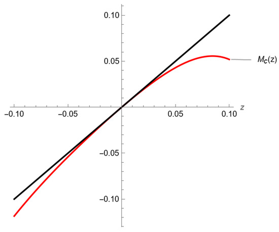
In Figure 5, we represent locally the graph of the function $M_c\left(z\right)$, generated using Mathematica [39].

Figure 5. The mapping $M_c$ from Example 3, restricted to the center manifold and represented in a neighborhood of the origin, along with its tangent line.

We compute $M_c\left(0\right)\approx 0$, $M_c^{\prime }\left(0\right)\approx 1$, and $M_c^{\prime \prime }\left(0\right)\approx -3.7419<0$. It then follows that the fixed point $z^{\ast }=0$ on the center manifold is semi-stable from the right. This conclusion is clearly seen in Figure 5. Consequently, the fixed point $(0, 0)$ of System (15) is semi-stable from the right. Thus, the carrying capacity $(x^{\ast }, u^{\ast })\approx (0.335743,-0.574966)$ of System (5) is semi-stable from the right.

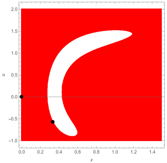
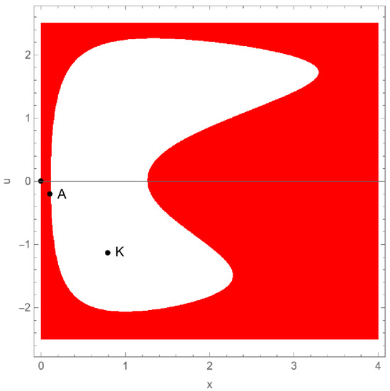
In Figure 6, we represent in the phase space the basins of attraction of both the origin (colored region) and the carrying capacity (non-colored region), generated using Mathematica [39].

Figure 6. The basin of attractions in the phase-space diagram of an example exhibiting a weak Allee effect. The parameter values are $c_0=1/2$, $c_1=2$, $s=4$, and ${\sigma }^2=4/5$. Initial conditions located in the colored region lead trajectories toward the origin; therefore, this region represents a basin of attraction of the origin. Given that ${\overline{b}}_0\approx 2.4037$, the carrying capacity is approximately $(x, u)\approx (0.335743,-0.574966)$. The basin of attraction of this equilibrium corresponds to the non-colored region.

As is clearly seen, the carrying capacity is semi-stable from the right. One can see that there exists a neighborhood U of $(x^{\ast }, u^{\ast })$, and a sectorial region $S\subset U$ (e.g., an angular sector), such that such that for every initial condition $(x_0, u_0)\in S$, the corresponding solution satisfies

$$\underset{t\to \infty }{lim}(x\left(t\right), u\left(t\right))=(x^{\ast }, u^{\ast }),$$

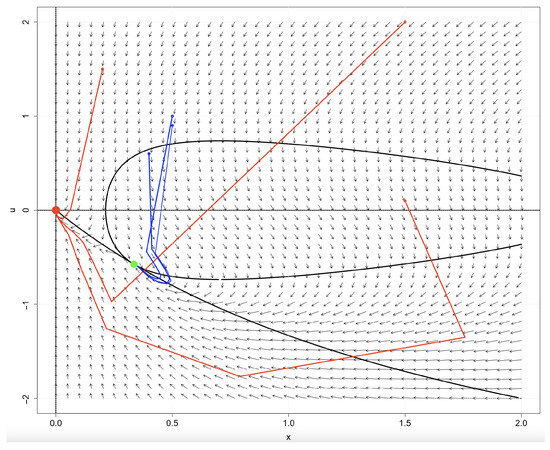
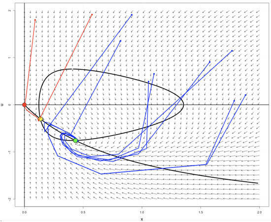
i.e., all trajectories starting in S converge to the carrying capacity, and there are initial conditions $(x_0,u_0)\in U\setminus S$ such that the corresponding trajectories not converge to $(x^{\ast },u^{\ast })$. This observation is clearly illustrated in Figure 7, generated using the software R 4.5.1. [40], which shows the orbits of selected initial points.

Figure 7. Selected orbits corresponding to initial points in the phase space for Example 3. The trajectories in blue converge to the interior equilibrium while the trajectories in red converge to the extinction equilibrium. The black curves represent the isoclines.

3.2.3. Strong Allee Effect

In this subsection, we consider that System (5) is under the influence of a strong Allee effect. This occurs when the parameter satisfies $b_0>{\overline{b}}_0$, where ${\overline{b}}_0$ is defined in Equation (11). In this case, there are two fixed points, which we denote by $\mathbf{A}=(x_A^{\ast },u_A^{\ast })$ and $\mathbf{K}=(x_K^{\ast },u_K^{\ast })$ where $x_A^{\ast }<x_K^{\ast }$. Following the literature, we refer to $\mathbf{A}$ as the Allee threshold and $\mathbf{K}$ as the carrying capacity.

The motivation for this terminology reflects the biological interpretation of the Allee effect: $\mathbf{A}$ marks the critical population threshold below which persistence is not possible, while $\mathbf{K}$ corresponds to the stable carrying capacity of the system. In the evolutionary System (5) under consideration here, $\mathbf{A}$ is indeed always unstable. However, similar to the case of a lone interior fixed point, $\mathbf{K}$ is only stable on a subset of ${\sigma }^2$ values, outside of which both of the nontrivial fixed points are unstable.

Our main result is the following:

Theorem 10. 

Let ${\overline{b}}_0$ be as defined in (11) and assume $b_0>{\overline{b}}_0$. Let $\mathbf{A}=(x_A^{\ast },u_A^{\ast })$ and $\mathbf{K}=(x_K^{\ast },u_K^{\ast })$ denote the Allee threshold point and carrying capacity respectively of System (5). Then for any ${\sigma }^2\in (0,2)$ the Allee threshold $\mathbf{A}$ is unstable. Further, there exists an interval $({\sigma }_{-},{\sigma }_{+})$ such that when ${\sigma }^2\in ({\sigma }_{-},{\sigma }_{+})$ the point $\mathbf{K}$ is locally asymptotically stable. Outside of this interval, the carrying capacity is unstable.

The remainder of this section is devoted to proving Theorem 10.

We recall that the Jacobian evaluated at any nontrivial fixed point of the mapping F associated with System (5) is given by

$$JF(x^{\ast },u^{\ast })=JF\left(x^{\ast },-{\displaystyle \frac{c_1{x}^{\ast }}{1+c_0{x}^{\ast }}}\right)=\left[\begin{array}{cc}{\displaystyle \frac{c_0{x}^{\ast }+s{x}^{\ast }+2}{\left(c_0{x}^{\ast }+1\right)\left(s{x}^{\ast }+1\right)}}& {\displaystyle \frac{c_1{\left(x^{\ast }\right)}^2}{c_0{x}^{\ast }+1}}\\ -{\displaystyle \frac{c_1{\sigma }^2}{{\left(c_0{x}^{\ast }+1\right)}^2}}& 1-{\sigma }^2\end{array}\right].$$

The determinant and the trace of the Jacobian are

$$Det\left(JF\right)={\displaystyle \frac{c_1^2{\sigma }^2{\left(x^{\ast }\right)}^2}{{\left(c_0{x}^{\ast }+1\right)}^3}}-{\displaystyle \frac{\left({\sigma }^2-1\right)\left(c_0{x}^{\ast }+s{x}^{\ast }+2\right)}{\left(c_0{x}^{\ast }+1\right)(s{x}^{\ast }+1)}}$$

and

$$Tr\left(JF\right)={\displaystyle \frac{c_0{x}^{\ast }+s{x}^{\ast }+2}{\left(c_0{x}^{\ast }+1\right)(s{x}^{\ast }+1)}}-{\sigma }^2+1.$$

Following the Jury’s criterion [41], one can determine the necessary and sufficient conditions for the roots of the characteristic polynomial of $JF(x^{\ast }, u^{\ast })$ to lie inside the unit circle. This occurs when $Det\left(JF\right)<1$, $Det\left(JF\right)>-Tr\left(JF\right)-1$ and $Det\left(JF\right)>Tr\left(JF\right)-1$. If at least one of these inequalities is reversed, then the fixed point is unstable.

We split the analysis of each of these three inequalities across the next three theorems.

Theorem 11. 

Let $0<{\sigma }^2\le 2$ and ${\overline{b}}_0$ be as defined in (11) and assume $b_0>{\overline{b}}_0$. Then the following inequality holds

$$Det\left(JF\right)>-Tr\left(JF\right)-1$$

for any nontrivial fixed point $(x^{\ast }, u^{\ast })$ of model (5).

Proof. 

A straightforward computation shows that:

$$\begin{array}{cc}\hfill Det\left(JF\right)+Tr\left(JF\right)+1& ={\displaystyle \frac{c_1^2{\sigma }^2{\left(x^{\ast }\right)}^2}{{(c_0{x}^{\ast }+1)}^3}}+{\displaystyle \frac{(2-{\sigma }^2)(c_0{x}^{\ast }+s{x}^{\ast }+2)}{(c_0{x}^{\ast }+1)(s{x}^{\ast }+1)}}-{\sigma }^2+2\hfill \\ \hfill & ={\displaystyle \frac{c_1^2{\sigma }^2{\left(x^{\ast }\right)}^2}{{(c_0{x}^{\ast }+1)}^3}}+{\displaystyle \frac{2-{\sigma }^2}{c_0{x}^{\ast }+1}}+{\displaystyle \frac{(2-{\sigma }^2)(s{x}^{\ast }+2)}{s{x}^{\ast }+1}}.\hfill \end{array}$$

Since $0<{\sigma }^2\le 2$, we have $2-{\sigma }^2\ge 0$, and all terms on the right-hand side are positive. Therefore,

$$Det\left(JF\right)+Tr\left(JF\right)+1>0,$$

which implies the desired inequality. □

Theorem 12. 

Let $0<{\sigma }^2<2$, and $\overline{x}$ and ${\overline{b}}_0$ be as defined in (11). Then $Det\left(JF\right)<Tr\left(JF\right)-1$ at $\mathbf{A}$ and $Det\left(JF\right)>Tr\left(JF\right)-1$ at $\mathbf{K}$.

Proof. 

We calculate

$$\begin{array}{cc}\hfill Det\left(JF\right)+1-Tr\left(JF\right)& ={\sigma }^2\left({\displaystyle \frac{c_1^2{\left(x^{\ast }\right)}^2}{{\left(c_0{x}^{\ast }+1\right)}^3}}-{\displaystyle \frac{c_0{x}^{\ast }+s{x}^{\ast }+2}{\left(c_0{x}^{\ast }+1\right)(s{x}^{\ast }+1)}}+1\right)\hfill \\ & ={\displaystyle \frac{{\sigma }^2\left(c_0^{3}s{x}^4+s(c_1^2+2c_0^2)x^3+(c_1^2-c_0^2+s{c}_0)x^2-2c_{0}x-1\right)}{{(c_0{x}^{\ast }+1)}^3(s{x}^{\ast }+1)}}\hfill \end{array}$$

where the bracketed portion of the numerator is the quartic from Theorem 1, which is negative when $x^{\ast }<\overline{x}$ and positive when $x^{\ast }>\overline{x}$. The remaining terms are all positive. From Theorem 1, we know $x_A^{\ast }<\overline{x}<x_K^{\ast }$ and the claim follows. □

Theorem 13. 

Let ${\overline{b}}_0$ be as defined in (11) and assume $b_0>{\overline{b}}_0$. Let $(x^{\ast }, u^{\ast })$ denote a nontrivial fixed point of System (5). Define

$${\widehat{x}}_{\ast }={\displaystyle \frac{c_0{x}^{\ast }+s{x}^{\ast }+2}{\left(c_0{x}^{\ast }+1\right)\left(s{x}^{\ast }+1\right)}},$$

$${\overline{x}}_{\ast }={\displaystyle \frac{c_1^2{\left(x^{\ast }\right)}^2}{{(c_0{x}^{\ast }+1)}^3}}$$

and

$${\sigma }_{\ast }={\displaystyle \frac{1-{\widehat{x}}_{\ast }}{{\overline{x}}_{\ast }-{\widehat{x}}_{\ast }}}$$

(where we define ${\sigma }_{\ast }=\infty$ if ${\overline{x}}_{\ast }={\widehat{x}}_{\ast })$.

Then we have the following:

1. 

If ${\sigma }_{\ast }\notin (0,2)$ and ${\widehat{x}}_{\ast }<1$, then $Det\left(JF\right)<1$ for ${\sigma }^2\in (0,2)$.

2. 

If ${\sigma }_{\ast }\in (0,2)$ and ${\widehat{x}}_{\ast }\le 1$, then $Det\left(JF\right)<1$ for ${\sigma }^2\in (0,{\sigma }^{\ast })$ and $Det\left(JF\right)\ge 1$ for ${\sigma }^2\ge {\sigma }^{\ast }$.

3. 

If ${\sigma }_{\ast }\in (0,2)$ and ${\widehat{x}}_{\ast }>1$, then $Det\left(JF\right)<1$ for ${\sigma }^2\in ({\sigma }^{\ast },2)$ and $Det\left(JF\right)\ge 1$ for ${\sigma }^2\le {\sigma }^{\ast }$.

4. 

If ${\sigma }_{\ast }\notin (0,2)$ and ${\widehat{x}}_{\ast }\ge 1$, then $Det\left(JF\right)\ge 1$ for ${\sigma }^2\in (0,2)$.

Proof. 

Observe that ${\overline{x}}_{\ast }$ and $\widehat{x_{\ast }}$ are independent of ${\sigma }^2$, and that

$$Det\left(JF\right)={\widehat{x}}_{\ast }+{\sigma }^2({\overline{x}}_{\ast }-{\widehat{x}}_{\ast }).$$

When viewed as a function of ${\sigma }^2$ alone, $Det\left(JF\right)$ is a line that is completely determined by the points $(0, {\widehat{x}}_{\ast })$ and $({\sigma }_{\ast }, 1)$. The location of these points implies the conclusion of the theorem. □

An illustration of the four cases in Theorem 13, generated using MATLAB [36], is shown in Figure 8. As shown in Theorem 13, the determinant is a straight line. The locations of $({\sigma }_{\ast },1)$ and $(0, {\widehat{x}}_{\ast })$ are shown. In all four plots, $c_0={\displaystyle \frac{1}{2}}$ and $s=4$. In the top plots, $c_1=2$, where in the top left $b_0={\displaystyle \frac{7}{2}}$ and in the top right $b_0=4$. On the bottom two plots, $c_1={\displaystyle \frac{5}{2}}$, and again $b_0={\displaystyle \frac{7}{2}}$ on the left and $b_0=4$ on the right. In each case, the location of $({\sigma }_{\ast },1)$ and $(0, \widehat{x})$ determines how much of the line segment for $Det\left(JF\right)$ lies below 1, as is needed for stability in the Jury conditions. In the plots, the line segment for $Det\left(JF\right)$ is extended beyond the interval $(0, 2)$ to better illustrate the location of $({\sigma }_{\ast }, 1)$, but ${\sigma }^2$ does not actually assume negative values.

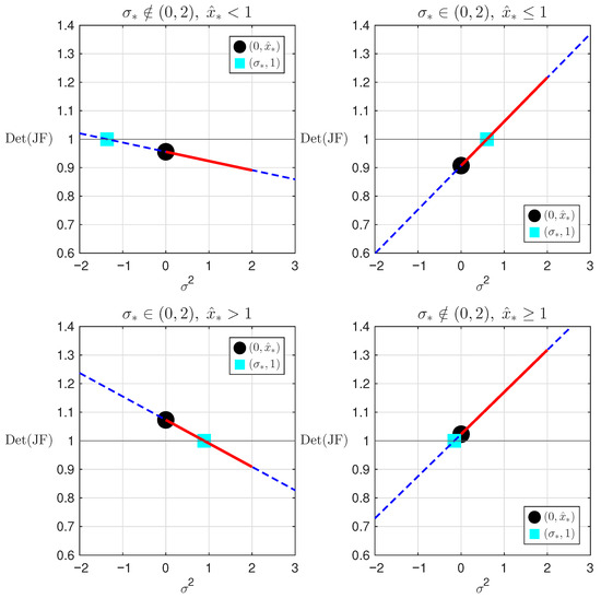
Figure 8. Graphs of $Det\left(JF\right)$ as a function of ${\sigma }^2$ for different parameter values.

We are now prepared to prove Theorem 10.

Proof of Theorem 10. 

From Theorem 1, we know $x_A^{\ast }<\overline{x}$. From Theorem 12, we know that at the fixed point $\mathbf{A}$ we have $Det\left(JF\right(\mathbf{A}\left)\right)<Tr\left(JF\right(\mathbf{A}\left)\right)-1$. Thus, from the Jury conditions, $\mathbf{A}$ is unstable.

For the fixed point $\mathbf{K}$, from Theorem 11, we know $Det\left(JF\right(\mathbf{K})>-Tr(JF\left(\mathbf{K}\right))-1$. From Theorem 12, we know that at the fixed point $\mathbf{K}$ we have $Det\left(JF\right(\mathbf{K}\left)\right)>Tr\left(JF\right(\mathbf{K}\left)\right)-1$. Finally, from Theorem 13, we know there is always an interval $({\sigma }_{-},{\sigma }_{+})$ for which $Det\left(JF\right(\mathbf{K}\left)\right)<1$ is satisfied for all ${\sigma }^2\in ({\sigma }_{-},{\sigma }_{+})$. Thus, from the Jury conditions, $\mathbf{K}$ is locally asymptotically stable provided ${\sigma }^2\in ({\sigma }_{-},{\sigma }_{+})$. □

Example 4. 

To illustrate our ideas, we consider a specific case with the following parameter values:

$$b_0=3.5,c_0=0.5,c_1=2\mathrm{and}s=4.$$

We focus on the cases where the evolutionary speed satisfies ${\sigma }^2\le 2$, since there is no convergence when ${\sigma }^2>2$, as the trajectory diverges and the trait equation becomes unbounded.

The fixed points are: the origin $\mathbf{O}$, the threshold Allee $\mathbf{A}=(0.111506,-0.211236)$, and the carrying capacity $\mathbf{K}=(0.792883,-1.13558)$.

From Theorem 4, we conclude that the origin $\mathbf{O}$ is locally asymptotically stable if $0<{\sigma }^2<2$. Its basin of attraction, generated using Mathematica [39], is shown in red in Figure 9 for ${\sigma }^2=0.9$. The orbit of any initial condition in this region converges to the trivial fixed point $\mathbf{O}$.

Figure 9. Basins of attraction of the origin $\mathbf{O}$ (red) and the carrying capacity $\mathbf{K}$ (white), using the parameter values from Example 4 and ${\sigma }^2=0.9$.

The Jacobian evaluated at the threshold point $\mathbf{A}$ is given by

$$JF\left(\mathbf{A}\right)=\left(\begin{array}{cc}1.63874& 0.0235541\\ -1.79434{\sigma }^2& 1-{\sigma }^2\end{array}\right)$$

whose eigenvalues are

$${\left({\lambda }_{\mathbf{A}}\right)}_{\pm }\left(\sigma \right)={\displaystyle \frac{1}{2}}\left(2.63874-{\sigma }^2\pm \sqrt{{\sigma }^4+1.10843{\sigma }^2+0.407991}\right).$$

It is clear that ${\sigma }^4+1.10843{\sigma }^2+0.407991>0$ for all $\sigma \in \mathbb{R}$, and that the functions ${\left({\lambda }_{\mathbf{A}}\right)}_{+}\left(\sigma \right)$ and ${\left({\lambda }_{\mathbf{A}}\right)}_{-}\left(\sigma \right)$ are increasing on the interval $\sigma \in [-\sqrt{2},0)$ and decreasing on the interval $\sigma \in (0,\sqrt{2}]$ so that $1.60631⪅{\left({\lambda }_{\mathbf{A}}\right)}_{+}\left(\sigma \right)⪅1.63874$ and $-1⪅{\left({\lambda }_{\mathbf{A}}\right)}_{-}\left(\sigma \right)⪅1$ for all $-\sqrt{2}\le \sigma \le \sqrt{2}$. Thus, the threshold point is unstable, more precisely a saddle fixed point.

At the carrying capacity $\mathbf{K}$ we have

$$JF\left(\mathbf{K}\right)=\left(\begin{array}{cc}0.955826& 0.90038\\ -1.02562{\sigma }^2& 1-{\sigma }^2\end{array}\right).$$

The eigenvalues of $JF\left(\mathbf{K}\right)$ are

$${\left({\lambda }_{\mathbf{K}}\right)}_{\pm }\left({\sigma }^2\right)={\displaystyle \frac{1}{2}}\left(1.95583-{\sigma }^2+\sqrt{{\sigma }^4-3.78212{\sigma }^2+0.00195135}\right).$$

For ${\sigma }^2\in (0,2)$ these two quantities are are complex conjugate whose absolute value is given by

$$\left|{\left({\lambda }_{\mathbf{K}}\right)}_{\pm }\left({\sigma }^2\right)\right|={\displaystyle \frac{1}{2}}\sqrt{3.8233-0.129531{\sigma }^2}.$$

Clearly, $|{\left({\lambda }_{\mathbf{K}}\right)}_{\pm }\left({\sigma }^2\right)|<1$ for any ${\sigma }^2\in (0,2)$. One can conclude that the carrying capacity $\mathbf{K}$ is locally asymptotically stable for any ${\sigma }^2\in (0,2)$. Its basin of attraction corresponds to the non-colored region in Figure 9 for ${\sigma }^2=0.9$.

In Figure 10, we show the orbits of several selected points in the phase space, generated using R 4.5.1. [40].

Figure 10. Selected orbits corresponding to initial points in the phase space for Example 4. The trajectories in blue converge to the interior equilibrium while the trajectories in red converge to the extinction equilibrium. The black curves represent the isoclines.

4. The Effect of Evolution

In this section, we analyze the impact of evolutionary processes on species x by comparing the dynamics of the Beverton–Holt type model with an Allee effect, both in the absence and presence of evolutionary dynamics. Specifically, we contrast the behavior of the model

$$x(t+1)={\displaystyle \frac{b_{0}s{x}^2\left(t\right)}{(1+c_{0}x\left(t\right))(1+sx\left(t\right))}}$$

(18)

with that of the evolutionary model described in Equation (5).

First, note that Equation (18) involves a reduced set of parameters, since it excludes the canonical equation of evolution. Consequently, the parameters related to evolutionary dynamics, such as the evolutionary speed and $c_1=c^{\prime }\left(0\right)$, do not appear; only $c_0=c\left(0\right)$ is present.

A direct analysis shows that if $b_0<{\widehat{b}}_0$, where

$${\widehat{b}}_0:={\displaystyle \frac{{(\sqrt{c_0}+\sqrt{s})}^2}{s}},$$

then the origin is the unique equilibrium of Equation (18). When $b_0={\widehat{b}}_0$, the model exhibits a weak Allee effect, with carrying capacity

$$\widehat{x}={\displaystyle \frac{1}{\sqrt{c_0}\sqrt{s}}}.$$

If $b_0>{\widehat{b}}_0$, the system is under the influence of a strong Allee effect, and two positive equilibria emerge:

$${\widehat{x}}_{\pm }={\displaystyle \frac{s(b_0-1)-c_0\pm \sqrt{{(s(b_0-1)-c_0)}^2-4s{c}_0}}{2s{c}_0}}.$$

Importantly, the condition $b_{0}s<{(\sqrt{c_0}+\sqrt{s})}^2$ for any $c_0\in (0,1)$, $s>0$, and $b_0>0$ implies global asymptotic stability of the origin in both models (Equation (5) with evolution and Equation (18) without evolution).

Biologically, the bifurcation points ${\widehat{b}}_0$ (in the non-evolutionary model) and ${\overline{b}}_0$ (in the evolutionary model) mark critical thresholds that separate qualitatively distinct population dynamics.

In both models, three ecological regimes are possible depending on the value of $b_0$: extinction, weak Allee effect, and strong Allee effect. When $b_0<{\widehat{b}}_0$ (or $b_0<{\overline{b}}_0$ in the evolutionary case), extinction is inevitable. At the threshold values $b_0={\widehat{b}}_0$ or $b_0={\overline{b}}_0$, the system undergoes a transcritical bifurcation, and the population may persist through a weak Allee effect. For $b_0$ exceeding the bifurcation point, the system enters a strong Allee effect regime, characterized by an unstable Allee threshold and a stable positive equilibrium.

Notably, one has ${\widehat{b}}_0<{\overline{b}}_0$, which means that the threshold for persistence is higher in the evolutionary model. Biologically, this implies that evolution may increase the demographic or environmental requirements necessary for population survival. While evolution can shape adaptive traits that benefit long-term persistence, it may also introduce constraints that delay recovery or increase extinction risk when reproductive output is low.

This structure reveals that evolution modifies the critical bifurcation point separating extinction and persistence. As a result, evolutionary dynamics may shift the conditions under which weak or strong Allee effects dominate, potentially expanding or restricting the environmental or demographic circumstances that enable population survival.

5. Conclusions

In this work, we investigated the global and evolutionary dynamics of discrete-time population models, with a focus on monotone and non-monotone maps under ecological pressures and evolutionary forces. By extending the classical Beverton-Holt framework (5), we introduced additional biological realism into the population dynamics through trait-based models that account for individual-level variation and its feedback on the population as a whole. Central to our study is the inclusion of a continuous heritable trait v, and the corresponding mean population trait u, whose dynamics are described in Equations (2) and (3).

We further incorporated Allee effects, both through mate limitation and predator saturation [3].

By embedding these into the Beverton-Holt framework [1], we revealed the presence of strong Allee effects, wherein persistence depends critically on initial conditions and trait distributions. Importantly, we showed conditions under which the coupled system (5) admits multiple attractors, including equilibria, cycles, and coexisting attractors.

Our results connect directly with eco-evolutionary models [3,10,11], and complement the epidemiological perspectives of Martcheva [42] and Brauer–Castillo-Chavez [43]. Together, these works underscore the need to unify evolutionary dynamics with epidemiological and ecological models, offering a richer framework for persistence and extinction under feedback-driven forces.

Future directions naturally extend from our system (5). Stochasticity, for example, can be added to either the demographic part (2) or the trait Equation (3), leading to new challenges in persistence and extinction analysis [42,44]. Non-autonomous forcing, whether periodic or almost periodic, will modify equilibria and bifurcation structures [45]. Multi-trait extensions of (3) open paths toward coevolutionary dynamics [10,11,46]. Structured systems combining (1) with age or spatial dispersal [21,38,43] may reveal multi-scale interactions between ecology, evolution, and epidemiology. Finally, numerical approaches adapted to (5) are required to detect global bifurcations and map basins of attraction in higher dimensions [37,41,47].

References

- Beverton, R.J.H.; Holt, S.J. On the dynamics of exploited fish populations. Fish. Investig. 1957, 19, 1–533. [Google Scholar]
- Leslie, P.H. Some further notes on the use of matrices in certain population mathematics. Biometrika 1948, 35, 213–245. [Google Scholar] [CrossRef]
- Elaydi, S.; Cushing, J.M. Discrete Mathematical Models in Population Biology; Springer: Berlin/Heidelberg, Germany, 2025. [Google Scholar]
- Elaydi, S.N. Discrete Chaos, 2nd ed.; Chapman & Hall/CRC: Boca Raton, FL, USA, 2007. [Google Scholar]
- Elaydi, S.N. An Introduction to Difference Equations, 3rd ed.; Springer: New York, NY, USA, 2005. [Google Scholar]
- Lande, R. Natural selection and random genetic drift in phenotypic evolution. Evolution 1976, 30, 314–334. [Google Scholar] [CrossRef]
- Lande, R. A quantitative genetic theory of life history evolution. Ecology 1982, 63, 607–615. [Google Scholar] [CrossRef]
- Abrams, P.A. Modelling the dynamics of life history evolution. Theor. Popul. Biol. 2001, 59, 345–357. [Google Scholar]
- D’Aniello, E.; Elaydi, S.; Kwessi, E.; Luís, R.; Ryals, B. Global Asymptotic Stability and Bifurcation of an Evolutionary Beverton-Holt Model. J. Differ. Equ. Appl. 2025, 1–39. [Google Scholar] [CrossRef]
- Dercole, F.; Rinaldi, S. Analysis of Evolutionary Processes; Princeton University Press: Princeton, NJ, USA, 2008. [Google Scholar]
- Brown, J.S.; Vincent, T.L. Evolutionary Game Theory, Natural Selection, and Darwinian Dynamics; Cambridge University Press: Cambridge, UK, 2005. [Google Scholar]
- Assas, L.; Dennis, B.; Elaydi, S.; Kwessi, E.; Livadiotis, G. A stochastic modified Beverton-Holt model with Allee effects. J. Differ. Equ. Appl. 2016, 22, 37–54. [Google Scholar] [CrossRef]
- Assas, L.; Elaydi, S.; Kwessi, E.; Livadiotis, G.; Ribble, D. Hierarchical competition models with Allee effect. J. Biol. Dyn. 2014, 9, 34–51. [Google Scholar] [CrossRef] [PubMed][Green Version]
- Assas, L.; Elaydi, S.; Kwessi, E.; Livadiotis, G.; Dennis, B. Hierarchical competition models with Allee effect II: The case of immigration. J. Biol. Dyn. 2015, 9, 288–316. [Google Scholar] [CrossRef]
- Courchamp, F.; Berec, L.; Gascoigne, J. Allee Effects in Ecology and Conservation; Oxford University Press: Oxford, UK, 2008. [Google Scholar]
- Cushing, J.M. The Allee effect in age-structured population dynamics. In Mathematical Ecology; Hallam, S.L.T., Gross, L., Eds.; Springer: Berlin, Germany, 1988; pp. 479–505. [Google Scholar]
- Cushing, J.M. Oscillations in age-structured population models with an Allee effect. J. Comput. Appl. Math. 1994, 52, 71–80. [Google Scholar] [CrossRef]
- Cushing, J.M. The evolutionary dynamics of a population model with a strong Allee effect. Math. Biosci. Eng. 2015, 12, 643–660. [Google Scholar] [CrossRef] [PubMed]
- Cushing, J.M. Difference equations as models of evolutionary dynamics. J. Biol. Dyn. 2019, 13, 103–127. [Google Scholar] [CrossRef] [PubMed]
- Elaydi, S.N.; Sacker, R.J. Population models with Allee effect: A new model. J. Biol. Dyn. 2010, 4, 397–408. [Google Scholar] [CrossRef]
- Livadiotis, G.; Assas, L.; Elaydi, S.; Kwessi, E.; Ribble, D. Competition models with Allee effects. J. Differ. Equ. Appl. 2014, 20, 1127–1151. [Google Scholar] [CrossRef]
- Livadiotis, G.; Elaydi, S. General Allee effect in two-species population biology. J. Biol. Dyn. 2012, 6, 959–973. [Google Scholar] [CrossRef]
- Ch-Chaoui, M.; Mokni, K. A discrete evolutionary Beverton–Holt population model. Int. J. Dyn. Control 2023, 11, 1060–1075. [Google Scholar] [CrossRef]
- Mokni, K.; Elaydi, S.; Ch-Chaoui, M.; Eladdadi, A. Discrete evolutionary population models: A new approach. J. Biol. Dyn. 2020, 14, 454–478. [Google Scholar] [CrossRef]
- Allee, W.C. Animal Aggregations: A Study in General Sociology; University of Chicago Press: Chicago, IL, USA, 1931. [Google Scholar] [CrossRef]
- Taylor, C.M. Allee Effects. In Encyclopedia of Theoretical Ecology; Hastings, A., Gross, L.J., Eds.; University of California Press: Berkeley, CA, USA, 2012; pp. 13–19. [Google Scholar] [CrossRef]
- Dennis, B. Allee effects: Population growth, critical density, and the Allee effect. Ecology 1989, 70, 1066–1072. [Google Scholar] [CrossRef]
- Adamson, P.T.; Morozov, A.Y. Bifurcation analysis of the predator–prey model with the Allee effect in the predator population. Math. Biol. 2021, 63, 1–24. [Google Scholar] [CrossRef]
- Ackleh, A.S.; Cushing, J.M.; Salceanu, P.L. On the dynamics of ecolutionary competition models. Nat. Resurce Model. 2015, 28, 380–397. [Google Scholar] [CrossRef]
- Cushing, J.M. An Evolutionary Beverton-Holt Model. In Theory and Applications of Difference Equations and Discrete Dynamical Systems; AlSharawi, E.S., Cushing, J.Z., Eds.; Springer Proceedings in Mathematics and Statistics; Springer: Berlin/Heidelberg, Germany, 2014. [Google Scholar]
- Cushing, J.M. A darwinian Ricker equation. In Progress on Difference Equations and Discrete Dynamical Systems; Baigent, S.E.S., Bhoner, M., Eds.; Springer Proceedings in Mathematics and Statistics; Springer: Cham, Switzerland, 2020; Volume 341, pp. 231–243. [Google Scholar]
- Mokni, K.; Ch-Chaoui, M. Strong Allee Effect and Evolutionary Dynamics in a Single-Species Ricker Population Model. J. Biol. Syst. 2023, 31, 1341–1370. [Google Scholar] [CrossRef]
- Mokni, K.; Ch-Chaoui, M. Exploring persistence, stability, and bifurcations: A Darwinian Ricker–Cushing model. Int. J. Dyn. Control 2025, 13, 34. [Google Scholar] [CrossRef]
- Mokni, K.; Ben, A.H.; Ghosh, B.; Ch-Chaoui, M. Nonlinear dynamics of a Darwinian Ricker system with strong Allee effect and immigration. Math. Comput. Simul. 2025, 229, 789–813. [Google Scholar] [CrossRef]
- Rael, R.C.; Vincent, T.L.; Cushing, J.M. Competitive outcomes changed by evolution. J. Biol. Dyn. 2011, 5, 227–252. [Google Scholar] [CrossRef]
- The MathWorks Inc. MATLAB, R2025a; The MathWorks, Inc.: Natick, MA, USA, 2025; Available online: https://www.mathworks.com (accessed on 1 June 2025).
- Carr, J. Applications of Center Manifold Theory; Springer: New York, NY, USA, 1982. [Google Scholar]
- Luís, R.; Elaydi, S.; Oliveira, H. Stability of a Ricker-type competition model and the competitive exclusion principle. J. Biol. Dyn. 2011, 5, 636–660. [Google Scholar] [CrossRef]
- Wolfram Research Inc. Mathematica, Version 14.3; Wolfram Research: Champaign, IL, USA, 2025; Available online: https://www.wolfram.com/mathematica/ (accessed on 1 June 2025).
- R Core Team. R: A Language and Environment for Statistical Computing; R Foundation for Statistical Computing: Vienna, Austria, 2024; Available online: https://www.R-project.org/ (accessed on 1 June 2025).
- Jury, E. On the roots of a real polynomial inside the unit circle and a stability criterion for linear discrete systems. IFAC Proc. Vol. 1963, 1, 142–153. [Google Scholar] [CrossRef]
- Martcheva, M. An Introduction to Mathematical Epidemiology; Springer: New York, NY, USA, 2015. [Google Scholar]
- Brauer, F.; Castillo-Chavez, C. Mathematical Models in Population Biology and Epidemiology, 2nd ed.; Springer: New York, NY, USA, 2012. [Google Scholar]
- Allen, L.J.S. An Introduction to Stochastic Processes with Applications to Biology; Prentice Hall: Upper Saddle River, NJ, USA, 2003. [Google Scholar]
- D’Aniello, E.; Elaydi, S. The structure of ω-limit sets of asymptotically non-autonomous discrete dynamical systems. DCDS-B 2020, 25, 903–915. [Google Scholar] [CrossRef]
- Hofbauer, J.; Sigmund, K. Evolutionary Games and Population Dynamics; Cambridge University Press: Cambridge, UK, 1998. [Google Scholar]
- Kot, M. Elements of Mathematical Ecology; Cambridge University Press: Cambridge, UK, 2001. [Google Scholar]
Disclaimer/Publisher’s Note: The statements, opinions and data contained in all publications are solely those of the individual author(s) and contributor(s) and not of MDPI and/or the editor(s). MDPI and/or the editor(s) disclaim responsibility for any injury to people or property resulting from any ideas, methods, instructions or products referred to in the content. |
© 2025 by the authors. Licensee MDPI, Basel, Switzerland. This article is an open access article distributed under the terms and conditions of the Creative Commons Attribution (CC BY) license (https://creativecommons.org/licenses/by/4.0/).