Limit Theorem for Kernel Estimate of the Conditional Hazard Function with Weakly Dependent Functional Data

Abstract

This paper examines the asymptotic behavior of the conditional hazard function using kernel-based methods, with particular emphasis on functional weakly dependent data. In particular, we establish the asymptotic normality of the proposed estimator when the covariate follows a functional quasi-associated process. This contribution extends the scope of nonparametric inference under weak dependence within the framework of functional data analysis. The estimator is constructed through kernel smoothing techniques inspired by the classical Nadaraya–Watson approach, and its theoretical properties are rigorously derived under appropriate regularity conditions. To evaluate its practical performance, we carried out an extensive simulation study, where finite-sample outcomes were compared with their asymptotic counterparts. The results showed the robustness and reliability of the estimator across a range of scenarios, thereby confirming the validity of the proposed limit theorem in empirical settings.

1. Introduction

Recent advances in computational technology and data acquisition systems have made it possible to store and process massive datasets that vary over time, including curves and images. These types of observations are commonly referred to as functional data. Effectively analyzing and modeling such data presents both a challenge and an opportunity for statisticians, leading to the development of powerful statistical tools—chief among them, nonparametric estimation methods.

Pioneering contributions by Bosq and Lecoutre [1], Ferraty and Vieu [2], Ferraty, Mas, and Vieu [3], and Laksaci and Mechab [4] laid the foundation for nonparametric estimation in the functional data context. Their works significantly influenced both the theoretical development and the practical implementation of kernel methods, making them key references in the field of nonparametric functional statistics.

Numerous researchers have addressed nonparametric models from both theoretical and practical perspectives. For instance, in the context of kernel estimation, Ferraty and Vieu [5], and Ferraty, Goia, and Vieu [6] investigated regression operators for functional data. Laksaci and Mechab [7] explored the asymptotic behavior of regression functions under weak dependence. Azzi et al. [8] presented functional modal regression for functional data, while Hyndman and Yao [9] proposed estimation techniques and symmetry tests for conditional density functions. Other notable contributions include those of Attaoui, Laksaci, and Ould Said [10], as well as Xu [11] and Abdelhak et al. [12], who investigated single-index models. Daoudi and Mechab [13] focused on estimating the conditional distribution function under quasi-association assumptions.

These contributions, centered on kernel-based methods for conditional models, provided significant insights into the asymptotic properties of estimators related to prediction, conditional distribution functions, and their derivatives, particularly conditional density. Furthermore, Bulinski and Suquet [14] examined random fields with both positive and negative dependence structures, Bouaker et al. [15] studied the consistency of the kernel estimator for conditional density in high-dimensional statistics, and Newman [16] investigated asymptotic independence and limit theorems in related settings.

With regard to the hazard function, several studies addressed its estimation in dependent contexts. Ferraty, Rabhi, and Vieu [17], Laksaci and Mechab [18], and Gagui and Chouaf [19] established asymptotic normality results under $\alpha$-mixing conditions.

The concept of $\alpha$-mixing (or strong mixing) is formalized through mixing coefficients, which quantify the degree of dependence between $\sigma$-algebras generated by collections of random variables that are increasingly separated in their index set (e.g., time, spatial locations, or other ordering dimensions). A stochastic process is said to be $\alpha$-mixing if these coefficients converge to zero as the separation increases. In this sense, $\alpha$-mixing imposes a strong form of asymptotic independence, ensuring that sufficiently distant observations behave nearly as independent random variables.

In contrast, quasi-association introduces a weaker and more flexible dependence structure, and was first introduced in [20] as a particular form of weak dependence. Rather than relying on the decay of mixing coefficients, quasi-association is defined through covariance inequalities involving monotone functions applied to disjoint subsets of variables (see Bulinski and Suquet, 2001 [21]). This framework controls dependence by bounding covariances, without requiring them to vanish completely, thereby accommodating a broader class of dependent random processes.

This distinction makes quasi-association particularly well-suited for the analysis of weakly dependent data, as it retains enough structure to establish central limit theorems while accommodating a broader class of stochastic processes than those encompassed by $\alpha$-mixing. Building on this framework, Kallabis and Neumann [22] derived exponential inequalities under weak dependence assumptions, further extending its theoretical foundations.

More recently, several studies have investigated nonparametric models involving quasi-associated random variables. Attaoui [23], Tabti and Ait Saidi [24], and Douge [25] also contributed to this line of research.

In addition, recent work has increasingly focused on the asymptotic analysis of conditional functional models under weak dependence structures, particularly quasi-association. Daoudi, Mechab, and Chikr Elmezouar [26], as well as Daoudi et al. [27], investigated the asymptotic properties of estimators of conditional hazard functions in single-index models for quasi-associated data. Similarly, Bouzebda, Laksaci, and Mohammedi [28] studied the single-index regression model, while Rassoul et al. [29] examined the MSE of the conditional hazard rate, highlighting its asymptotic behavior under weak dependence. Daoudi et al. [30] demonstrated asymptotic results of a conditional risk function estimator for associated data in high-dimensional statistics.

In this context, further contributions strengthened the theoretical foundation of kernel-based nonparametric estimators. High-dimensional statistics and complex dependence frameworks have also been explored in the literature. For instance, some works considered the asymptotic behavior of regression estimators under quasi-associated functional time series [31]. These works confirm the growing interest in developing robust asymptotic results for conditional models with dependent functional data, providing theoretical tools that support practical applications.

While the asymptotic behavior of hazard function estimators has been studied under independence or classical mixing conditions, much less attention has been given to functional data subject to weak dependence. In particular, the quasi-association structure—common in many real-world settings such as spatial or temporal processes—remains underexplored in the context of nonparametric hazard estimation.

This study addresses this gap by examining the asymptotic characteristics of the conditional hazard function estimator for functional data under quasi-association, with the aim of establishing its asymptotic properties. We begin by introducing the functional model together with the necessary notation and mathematical tools. As a first result, we establish almost complete consistency. Then, we derive asymptotic normality by employing analytical techniques and decomposition strategies. All theoretical developments are supported with rigorous proof.

To validate the theoretical findings, we conduct a numerical study demonstrating the asymptotic normal approximation of the proposed estimator. Specifically, we generate three datasets of different sizes to examine the impact of key parameters such as sample size and bandwidth on estimator performance. Graphical comparisons between theoretical and empirical results illustrate the estimator’s effectiveness and assess the quality of the estimation.

Beyond its theoretical contribution, the proposed estimator also has practical significance. In medical survival analysis, it can be used to model patient lifetimes where spatial or functional dependencies naturally arise. In reliability engineering, it offers a tool for evaluating the failure times of complex systems with dependent components. Moreover, in risk assessment involving spatially correlated data, such as environmental or epidemiological studies, our approach provides a more realistic framework than classical independence-based methods. These applications highlight the relevance of our theoretical results in addressing real-world problems.

The remainder of this paper is structured as follows. Section 2 presents the quasi-associated sequence, outlines the model construction, and introduces the estimator. Section 3 states the necessary assumptions and develops the results concerning almost complete convergence and asymptotic normality of the estimator. Section 4 provides a comprehensive numerical study supporting the theoretical findings and offering asymptotic confidence bounds. The conclusion synthesizes the key findings and highlights potential directions for future research. Finally, detailed proofs of the main results are given in Appendix A.

2. The Model

Let $Z_i={(S_i,T_i)}_{1\le i\le n}$, be an $\mathcal{H}\times \mathbb{R}$-valued measurable and strictly stationary stochastic process defined on a probability space $(\mathsf{\Omega },\mathcal{A},\mathbb{P})$, where $(\mathcal{H},d)$ denotes a semi metric space, where $\mathcal{H}$ is a normed $\Vert .\Vert$ Hilbert space, provided with an inner product $<.,.>$.

In the following, we consider a fixed point $s\in \mathcal{H}$ and denote by ${\mathcal{N}}_s$ a fixed neighborhood of s. In addition, let $\mathcal{S}$ be a fixed compact subset of $\mathbb{R}$, corresponding to the support of the time variable T. The notation s refers to an element of the functional space $\mathcal{H}$, whereas $\mathcal{S}$ denotes a compact subset of $\mathbb{R}$.

The semi metric noted d defined by $d(s,s^{\prime })=\Vert s-s^{\prime }\Vert ,\forall s,s^{\prime }\in \mathcal{H}$. We consider a fixed point s in $\mathcal{H}$, ${\mathcal{N}}_s$ a fixed neighborhood of s and $\mathcal{S}$ be a fixed compact subset of $\mathbb{R}$. We assume the existence of a regular version of the conditional probability distribution of the random variable T given S. Furthermore, for all ${\mathcal{N}}_s$, we suppose that the conditional distribution function of T given $S=s$ denoted by $G^s(·)$ is three times continuously differentiable. We denote its corresponding conditional density function by $g^s(·)$.

In this paper, we investigate the kernel estimation of the conditional hazard function of T given $S=s$, denoted ${\lambda }^s\left(t\right)$, for all $t\in \mathbb{R}$ such that $G^s\left(t\right)<1$, is given by

$${\lambda }^s\left(t\right)={\displaystyle \frac{g^s\left(t\right)}{1-G^s\left(t\right)}}.$$

In our functional context, the kernel estimate of this function is given by

$$\begin{array}{c}\hfill {\widehat{\lambda }}^s\left(t\right)={\displaystyle \frac{{\widehat{g}}^s\left(t\right)}{1-{\widehat{G}}^s\left(t\right)}},\forall t\in \mathbb{R},\end{array}$$

(1)

where ${\widehat{G}}^s(·)$ is the conditional distribution functional estimator, given by

$$\begin{array}{c}\hfill {\widehat{G}}^{·}\left(t\right)={\displaystyle \frac{{\sum }_{i=1}^{n}K\left({\theta }_K^{-1}d\left(·,S_i\right)\right)H\left({\theta }_H^{-1}\left(t-T_i\right)\right)}{{\sum }_{i=1}^{n}K\left({\theta }_K^{-1}d\left(·,S_i\right)\right)}},\forall t\in \mathbb{R}\end{array}$$

(2)

and ${\widehat{g}}^s(·)$ is the conditional density functional estimator, given by

$$\begin{array}{c}\hfill {\widehat{g}}^{·}\left(t\right)={\displaystyle \frac{{\sum }_{i=1}^{n}K\left({\theta }_K^{-1}d\left(·,S_i\right)\right)H^{\prime }\left({\theta }_H^{-1}\left(t-T_i\right)\right)}{{\sum }_{i=1}^{n}K\left({\theta }_K^{-1}d\left(·,S_i\right)\right)}},\forall t\in \mathbb{R}.\end{array}$$

(3)

With K denote a kernel function, H be a given differentiable distribution function with derivative $H^{\prime }$. The quantities ${\theta }_K={\theta }_{K,n}$ and ${\theta }_H={\theta }_{H,n}$ represent sequences of positive bandwidth parameters. Under this framework, the estimator ${\widehat{\lambda }}^s\left(t\right)$ can be expressed as

$${\widehat{\lambda }}^s\left(t\right)={\displaystyle \frac{{\widehat{g}}_N^s\left(t\right)}{{\widehat{G}}_D^s-{\widehat{G}}_N^s\left(t\right)}}.$$

(4)

where

$$\begin{array}{cc}\hfill {\widehat{G}}_D^{·}& ={\displaystyle \frac{1}{n\mathbb{E}\left[K_1(·)\right]}}\sum _{i=1}^n{K}_i(·)\hfill \\ \hfill {\widehat{G}}_N^{·}\left(t\right)& ={\displaystyle \frac{1}{n\mathbb{E}\left[K_1(·)\right]}}\sum _{i=1}^n{K}_i(·)H_i\left(t\right)\hfill \\ \hfill {\widehat{g}}_N^{·}\left(t\right)& ={\displaystyle \frac{1}{n{h}_H\mathbb{E}\left[K_1(·)\right]}}\sum _{i=1}^n{K}_i(·)H_i^{\prime }\left(t\right)\hfill \end{array}$$

(5)

with notational convenience:

$$K_i(·)=K\left({\theta }_K^{-1}d\left(·,S_i\right)\right),\mathrm{and}{H}_i\left(t\right)=H\left({\theta }_H^{-1}\left(t-T_i\right)\right).$$

Our primary objective is to establish both the consistency and the asymptotic normality of the estimator (4) under suitable hypothesis, where the sequence of variables ${\left(S_n\right)}_{n\in \mathbb{N}}$ verify the quasi-association as defined by Bulinski and Suquet [14].

Definition 1.

Let $I_1$ and $I_2$ be disjoint subsets of $\mathbb{N}$, i.e., $I_1\cap I_2=⌀$. For all Lipschitz functions

$$f_1:{\mathbb{R}}^{|I_1|d}\to \mathbb{R},f_2:{\mathbb{R}}^{|I_2|d}\to \mathbb{R},$$

the sequence ${\left(S_n\right)}_{n\in \mathbb{N}}$, with $S_n\in {\mathbb{R}}^d$, is said to be quasi-associated if

$$\begin{array}{c}\hfill Cov\left(f_1(S_{\tau },\tau \in I_1),f_2(S_{\kappa },\kappa \in I_2)\right)\le Lip\left(f_1\right)Lip\left(f_2\right)\sum _{\tau \in I_1}\sum _{\kappa \in I_2}\sum _{u=1}^d\sum _{v=1}^d|Cov(S_{\tau }^u,S_{\kappa }^v)|,\end{array}$$

where

$$Lip\left(f_1\right)=\underset{s\ne t}{sup}{\displaystyle \frac{|f_1\left(s\right)-f_1\left(t\right)|}{\parallel s-t\parallel }},\parallel (s_1,\dots ,s_n)\parallel =|s_1|+\cdots +|s_n|.$$

Here, $S_{\tau }^u$ denotes the u-th component of $S_{\tau }$, i.e., $S_{\tau }^u:=⟨S_{\tau },e_u⟩$, with ${\left(e_u\right)}_{u\ge 1}$ an orthonormal basis.

Finally, the pair ${{\rm Y}}_l=\{(S_{\tau },h_{\tau }),\tau \in \mathbb{N}\}$ is referred to as a stationary quasi-associated process.

3. Main Results

3.1. Assumptions

In the sequel, when no confusion will likely to arise, we will denote by $\alpha$ and ${\alpha }^{\prime }$ strictly positive constants, and by ${\chi }_u$ the covariance coefficient defined as

$$\begin{array}{c}\hfill {\chi }_u=su{p}_{v\ge u}\sum _{|i-j|\ge v}{\chi }_{i,j}\end{array}$$

where

$$\begin{array}{c}\hfill {\chi }_{i,j}=\sum _{u\ge 1}\sum _{v\ge 1}|Cov(S_i^u,S_j^v)|+\sum _{u\ge 1}|Cov(S_i^u,T_j)|+\sum _{v\ge 1}|Cov(T_i,S_j^v)|+|Cov(T_i,T_j)|.\end{array}$$

$S_i^u$ denotes The $uth$ component of $S_i$, where $S_i^u:=<S_i,e_u>$.

For $\rho >0$, let $B(s,\rho ):=\{s^{\prime }\in \mathcal{H}/d(s,s^{\prime })<\rho \}$ be a small ball, s is its center and $\rho$ is its radius.

To achieve the desired goal, we begin by stating the following required assumptions.

($H_1$)

$\mathbb{P}(S\in B(s,{\theta }_K))={\varphi }_s\left({\theta }_K\right)>0$, and ${\varphi }_s(·)$ is a differentiable at 0.

Moreover, $\exists {\beta }_s(·)$ such that $\forall u\in [-1,1]:$

${\displaystyle \underset{{\theta }_K\to 0}{lim}\frac{{\varphi }_s\left(u{\theta }_K\right)}{{\varphi }_s\left({\theta }_K\right)}={\beta }_s\left(u\right).}$

($H_2$)

Assume that the Hölder continuity condition holds for both functions $G^s\left(t\right)$ and $g^s\left(t\right)$.

$$\begin{array}{cc}\hfill \left|G^{s_1}\left(t_1\right)-G^{s_2}\left(t_2\right)\right|& \le \gamma \left(d^{{\gamma }_1}(s_1,s_2)+{|t_1-t_2|}^{{\gamma }_2}\right)\hfill \\ \hfill \left|g^{s_1}\left(t_1\right)-g^{s_2}\left(t_2\right)\right|& \le {\gamma }^{\prime }\left(d^{{\gamma }_1}(s_1,s_2)+{|t_1-t_2|}^{{\gamma }_2}\right)\hfill \end{array}$$

for all $(s_1,s_2)\in {\mathcal{N}}_s^2$ and $(t_1,t_2)\in {\mathcal{S}}^2$, with constants $\gamma >0$, ${\gamma }^{\prime }>0$, and $\mathcal{S}$ be a subset of $\mathbb{R}$ ($\mathcal{S}$ compact).

($H_3$)

$H^{\prime }$ is even, bounded, and Lipschitz continuous, and it satisfies

$${\int }_{\mathbb{R}}{H}^{\prime }\left(z\right)dz=1,{\int }_{\mathbb{R}}{\left|z\right|}^{{\gamma }_2}{H}^{\prime }\left(z\right)dz<\infty ,\mathrm{and}{\int }_{\mathbb{R}}{\left(H^{\prime }\left(z\right)\right)}^{2}dz<\infty .$$

($H_4$)

For a differentiable, Lipschitz continuous and bounded kernel K, $\exists \eta$ and ${\eta }^{\prime }$ so that

$$\begin{array}{c}\hfill \eta {\mathbb{I}}_{[0,1]}(·)<K(·)<{\eta }^{\prime }{\mathbb{I}}_{[0,1]}(·)\end{array}$$

with

$$-\infty <\eta <K^{\prime }\left(z\right)<{\eta }^{\prime }<0\mathrm{for}0\le z\le 1.$$

($H_5$)

The random pairs $(S_{\kappa },T_{\kappa }),\kappa \in \mathbb{N}$ form a quasi-associated sequence with covariance coefficient ${\chi }_u$, $u\in \mathbb{N}$ satisfying the following:

$$\begin{array}{c}\hfill \exists a>0,\exists \kappa >0,\mathrm{such}\mathrm{that}{\chi }_u\le \kappa e^{-au}.\end{array}$$

($H_6$)

$$\begin{array}{cc}\hfill {\displaystyle 0<\underset{i\ne j}{sup}\mathbb{P}\left[(S_i,S_j)\in B(s,{\theta }_K)\times B(s,{\theta }_K)\right]}& =\underset{i\ne j}{max}\left\{\mathbb{P}\left(d\left(s,S_i\right)<{\theta }_K\right),\mathbb{P}\left(d\left(s,S_j\right)<{\theta }_K\right)\right\}\hfill \\ \hfill & =O\left({\varphi }_s^2\left({\theta }_K\right)\right).\hfill \end{array}$$

($H_7$)

The bandwidths ${\theta }_K$ and ${\theta }_H$ satisfy

i-

$$\underset{n\to \infty }{lim}{\displaystyle \frac{1}{n{\theta }_H{\varphi }_s\left({\theta }_K\right)}}=0,\underset{n\to \infty }{lim}{\displaystyle \frac{{log}^{5}n}{n{\theta }_H{\varphi }_s\left({\theta }_K\right)}}=0.$$

ii-

$$\underset{n\to \infty }{lim}n{\theta }_H^5{\varphi }_s\left({\theta }_K\right)=0,\underset{n\to \infty }{lim}n{\theta }_H^2{\theta }_K{\varphi }_s\left({\theta }_K\right)=0.$$

iii-

$$\underset{n\to \infty }{lim}\left({\theta }_H^2+{\theta }_K\right)\sqrt{n{\varphi }_s\left({\theta }_K\right)}=0.$$

($H_8$)

For $m\in \{0,2\}$, the functions

$${\mathsf{\Phi }}_l(·)=\mathbb{E}\left[{\displaystyle \frac{{\partial }^m{g}^S\left(t\right)}{\partial t^m}}-{\displaystyle \frac{{\partial }^m{g}^s\left(t\right)}{\partial t^m}}|d(s,S)=·\right]$$

and

$$\Psi (·)=\mathbb{E}\left[{\displaystyle \frac{{\partial }^m{G}^S\left(t\right)}{\partial t^m}}-{\displaystyle \frac{{\partial }^m{G}^s\left(t\right)}{\partial t^m}}|d(s,S)=·\right]$$

are differentiable at 0.

3.2. Comments on the Assumptions

We classify the assumptions into standard ones commonly used in the nonparametric functional literature and those that are specific or new in the context of quasi-associated functional data:

($H_1$)

Specific to this paper. This assumption specifies conditions governing the probability that S lies within a neighborhood of s, along with the limiting behavior of the corresponding probability ratio as the neighborhood size approaches zero. These conditions are essential for the asymptotic analysis under quasi-association.

($H_2$)

Standard. The Hölder continuity imposed on the conditional distribution $G^s\left(t\right)$ and its density $g^s\left(t\right)$ is a classical regularity condition ensuring smoothness and enabling uniform convergence arguments.

($H_3$)

Standard. Conditions on the kernel H (even, bounded, with bounded Lipschitz derivative) are standard in kernel estimation to ensure proper convergence of the estimator.

($H_4$)

Standard. Properties of the kernel K (bounded, differentiable, indicator bounds) are classical technical assumptions required for Taylor expansions and bias control.

($H_5$)

Specific to this paper. The quasi-association assumption on the sequence $\left\{(S_{\kappa },T_{\kappa })\right\}$ generalizes independence or classical mixing conditions, allowing us to treat weak spatial dependence in functional data.

($H_6$)

Specific to this paper. This condition characterizes the asymptotic behavior of the joint probability of two functional covariates in neighborhoods of s, controlling covariance terms in the asymptotic expansions under quasi-association.

($H_7$)

Standard. Bandwidth conditions for ${\theta }_K$ and ${\theta }_H$ are classical in nonparametric functional estimation to balance bias and variance.

($H_8$)

Specific to this paper. This assumption concerns the differentiability at 0 of certain conditional expectation functions. It is required for precise control of higher-order terms in the asymptotic analysis under quasi-association.

3.3. The Almost Consistency

Our goal is to derive the almost complete convergence (a.co.) of ${\widehat{\lambda }}^s\left(t\right)$ to ${\lambda }^s\left(t\right)$, and this result is formalized in the following theorem.

Theorem 1.

Under the conditions ($H_1$)–($H_8$), we have

$$\begin{array}{c}\hfill \left|\widehat{{\lambda }^s}\left(t\right)-{\lambda }^s\left(t\right)\right|=O\left({\theta }_H^2+{\theta }_K\right)+O_{\mathrm{a}.\mathrm{co}.}\left(\sqrt{{\displaystyle \frac{logn}{n{\theta }_H{\varphi }_s\left({\theta }_K\right)}}}\right)\mathit{as}n\to \infty .\end{array}$$

3.4. Asymptotic Normality

Theorem 2.

Under ($H_1$)–($H_7$), we infer

$$\sqrt{n{\theta }_H{\varphi }_s\left({\theta }_K\right)}\left({\widehat{\lambda }}^s\left(t\right)-{\lambda }^s\left(t\right)\right)\stackrel{\mathcal{D}}{\to }\mathcal{N}\left(0,{\sigma }_{\widehat{\lambda }}^2\right),\forall s\in \mathcal{A};n\to \infty ,$$

where

$$\begin{array}{cc}\hfill \mathcal{A}=& \left\{s\in \mathcal{H},g^s\left(t\right)\left(1-G^s\left(t\right)\right)\ne 0\right\},\hfill \end{array}$$

with

$${\sigma }_{\widehat{\lambda }}^2={\displaystyle \frac{{\omega }_2{\lambda }^s\left(t\right)}{{\omega }_1^2\left(1-G^s\left(t\right)\right)}}\int {\left(H^{\prime }\left(u\right)\right)}^{2}du.$$

$${\omega }_{\tau }=K^{\tau }\left(1\right)-{\int }_0^1{\left(K^{\tau }\right)}^{\prime }\left(u\right){\beta }_s\left(u\right)du,\mathit{for}\tau =1,2.$$

The complete proofs of Theorems 1 and 2 are given in Appendix A.

4. Application and Numerical Study

4.1. Confidence Bounds

Constructing reliable confidence bounds is a key aspect of statistical analysis, as they characterize the variability and reliability of model estimators. Proper interpretation of these bounds enables more informed and robust conclusions about the underlying estimator. In the context of survival and hazard function estimation, confidence bounds are particularly valuable since they provide a quantitative assessment of the uncertainty surrounding the estimated conditional hazard function, thereby guiding both theoretical analysis and practical decision-making. Moreover, confidence bounds serve as a diagnostic tool: narrow bounds suggest stable and precise estimators, while wider bounds highlight regions where the estimator is less reliable due to limited data or high variability.

As an application of the result established in Theorem 2, we construct confidence bounds for ${\lambda }^s\left(t\right)$ at the confidence level $1-\alpha$. To this end, we must first estimate the unknown components of the asymptotic variance as follows: these include the conditional density, the conditional survival function, and kernel-based quantities that appear in the variance expression. Consistent estimation of these components is essential, since any bias or misspecification would directly affect the coverage probability of the resulting bounds. Once these quantities are estimated, the asymptotic normality result in Theorem 2 allows us to approximate the distribution of the estimator and derive pointwise confidence intervals for ${\lambda }^s\left(t\right)$ across the range of t. This methodology not only validates the theoretical properties of the proposed estimator but also ensures its applicability in empirical studies where inference on the conditional hazard function is required.

$${\widehat{\omega }}_q=:{\displaystyle \frac{1}{n{\widehat{\varphi }}_s\left({\theta }_K\right)}}\sum _{\tau =1}^n{K}_{\tau }^q,q=1,2;$$

$${\widehat{\varphi }}_s\left({\theta }_K\right)={\displaystyle \frac{\#\left\{\tau :\left|d\left(S_{\tau },s\right)\right|\le {\theta }_K\right\}}{n}},$$

where $\#\left(A\right)$ represents the cardinality of the set A. Also, ${\sigma }_{\widehat{\lambda }}^2$ is estimated by

$$\widehat{{\sigma }_{\widehat{\lambda }}^2}=:{\displaystyle \frac{\widehat{{\omega }_2}{\widehat{\lambda }}^s\left(t\right)}{{\widehat{\omega }}_1^2}}\int {\left(H^{\prime }\left(u\right)\right)}^{2}du.$$

(6)

Corollary 1.

When the assumptions of Theorem 2 hold, we set

$$\sqrt{n{\theta }_H{\widehat{\varphi }}_s\left({\theta }_K\right)}\left({\widehat{\lambda }}^s\left(t\right)-{\lambda }^s\left(t\right)\right)\stackrel{d}{⟶}N\left(0,\widehat{{\sigma }_{\widehat{\lambda }}^2}\right),n\to \infty .$$

(7)

Moreover, the confidence bounds will be,

$$\left[{\widehat{\lambda }}^s\left(t\right)-Z_{1-{\displaystyle \frac{\alpha }{2}}}{\left({\displaystyle \frac{\widehat{{\sigma }_{\widehat{\lambda }}^2}}{n{\theta }_H{\widehat{\varphi }}_s\left({\theta }_K\right)}}\right)}^{1/2},{\widehat{\lambda }}^s\left(t\right)+Z_{1-{\displaystyle \frac{\alpha }{2}}}{\left({\displaystyle \frac{\widehat{{\sigma }_{\widehat{\lambda }}^2}}{n{\theta }_H{\widehat{\varphi }}_s\left({\theta }_K\right)}}\right)}^{1/2}\right],$$

where $Z_{1-{\displaystyle \frac{\alpha }{2}}}$ is the quantile $1-{\displaystyle \frac{\alpha }{2}}$ of $\mathcal{N}(0,1)$.

4.2. Numerical Study

In this part, we conduct a numerical study using R software to illustrate and validate the theoretical results through graphical representations. The aim of this simulation is to assess the finite-sample performance of the proposed estimator and to highlight the extent to which the asymptotic properties established in the theoretical framework are reflected in practice. By generating controlled data under specific dependence structures and censoring mechanisms, we are able to visualize the behavior of the conditional density and hazard estimators, compare them with their theoretical counterparts, and evaluate their accuracy across different sample sizes. This numerical experiment also provides insights into the rate of convergence, the influence of the smoothing parameters, and the robustness of the estimator under varying conditions.

This simulation is based on the following points: We describe the data-generating process and the dependence structure imposed, specify the choice of kernel functions and bandwidths, outline the implementation of the random censoring mechanism, and finally present the graphical outputs and error metrics that allow for a systematic comparison between theoretical and empirical curves. The numerical results obtained will not only complement the theoretical findings but also serve as practical evidence of the efficiency and reliability of the proposed estimation methodology.

• Define our model by choosing functional covariate as

  $$S_{\kappa }\left(u\right)=cos\left(W_{\kappa }u\right)+sin\left(W_{\kappa }+u\right)+0.7\left(W_{\kappa }u\right),u\in [0,+\pi ]\mathrm{for}\kappa =1,\dots ,n$$
  The choice of the model $S_{\kappa }\left(u\right)$ is motivated by both theoretical and practical considerations. First, it adequately reflects the main characteristics of real functional data, in particular smoothness and variability, which are essential features in many applied contexts. Second, its structure makes it sufficiently flexible to mimic realistic scenarios while remaining simple enough to allow rigorous analysis within the framework of our simulation study.
  The process $\left(W_{\kappa }\right)$ satisfies a specific dependence structure, namely a quasi-associated sequence, which is generated as a non-strong mixing auto-regressive process of order 1.
  The choice of the model is constructed by setting the auto-regressive coefficient $\rho =0.1$ and modeling the innovation term as a binomial distribution $\mathrm{Binom}(10,0.25)$ [17]. We use 100 discretization points of u to obtain the curves $S_{\kappa }$ shown below in Figure 1, Figure 2 and Figure 3, corresponding to different sample sizes.
  

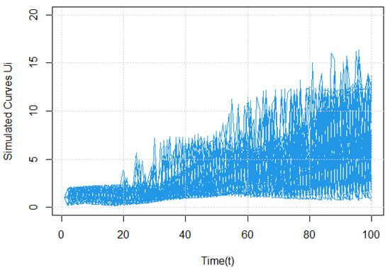  Figure 1. Simulated sample paths $S_{\kappa =1,\dots ,n}$ of the quasi-associated AR(1) process with $n=50$.
  

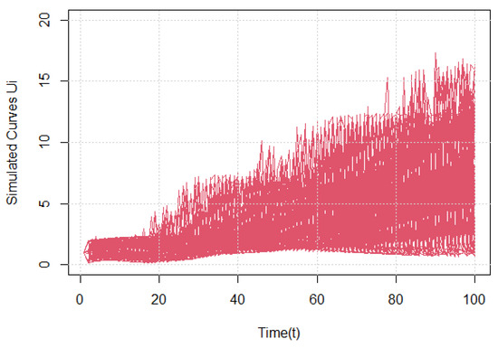  Figure 2. Simulated sample paths $S_{\kappa =1,\dots ,n}$ of the quasi-associated AR(1) process with $n=200$.
  

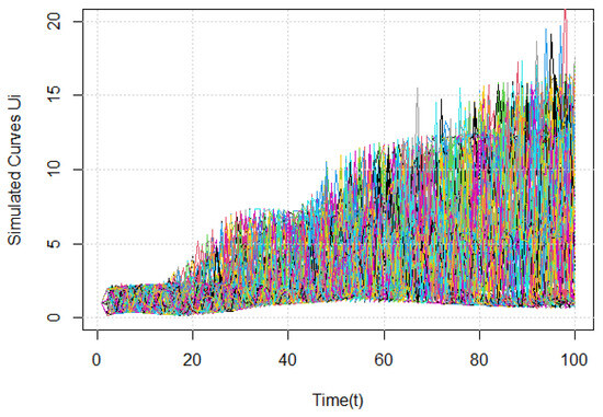  Figure 3. Simulated sample paths $S_{\kappa =1,\dots ,n}$ of the quasi-associated AR(1) process with $n=1000$.
  The real variable is defined as $T=m\left(S\right)+ϵ$. Where m is the nonlinear regression operator,

  $$m\left(S\right)={\displaystyle \frac{1}{5}}\times exp\left\{2-{\displaystyle \frac{1}{{\left({\int }_0^{\pi }{S}^{\prime }\left(u\right)du\right)}^2}}\right\}$$

  and $ϵ$ is distributed as standard normal distribution. It is clear that the explicit form of the conditional density given by

  $$g^s\left(t\right)={\displaystyle \frac{1}{\sqrt{2\pi }}}{\mathrm{e}}^{-{\displaystyle \frac{1}{2}}{\left(t-m\left(s\right)\right)}^2}.$$
  In the next, we select the distance in $\mathcal{H}$ as

  $$d\left(s_1,s_2\right)={\left({\int }_0^{\pi }{\left(s_1^{\prime }\left(u\right)-s_2^{\prime }\left(u\right)\right)}^{2}du\right)}^{1/2}\forall s_1,s_2\in \mathcal{H}.$$
  Also

  $$K\left(s\right)={\displaystyle \frac{15}{16}}{\left(1-s^2\right)}^2,s\in [-1,1];H\left(s\right)={\int }_{-\infty }^{s}K\left(u\right)du.$$
• A bandwidth selection algorithm: The smoothness of the estimators (2) and (3) is controlled by the smoothing parameter ${\theta }_K$ and the regularity of the cumulative distribution function. Therefore, choosing these parameters plays a critical role in the computational process.
  An optimal selection leads to effective estimation with a small mean squared error, which, for the conditional hazard function, is given by

  $$MSE\left(\widehat{\lambda }\right)={\displaystyle \frac{1}{n}}\sum _{i=1}^n{\left({\widehat{\lambda }}^s\left(t_i\right)-{\lambda }^s\left(t_i\right)\right)}^2.$$
  Let $H(.)$ be a distribution function on $\mathbb{R}$ and $H_{\theta }\left(s\right)=H(s/\theta )$. Note that as $\theta \to 0$.

  $$\mathbb{E}\left\{H_{\theta }\left(t-T_i\right)|S_i=s\right\}=G^s\left(t\right)+O\left({\theta }^2\right).$$
  This result shows that $G^s\left(t\right)$ can be interpreted as the regression of $H_{\lambda }(t-T_i)$ on $S_i$. Consequently, we adopt this regression framework for our estimation problem. By combining this approach with the normal reference rule [7], we obtain a practical algorithm for selecting the bandwidth parameters:

  i

  Compute the bandwidth ${\theta }_H$ using the normal reference rule.

  ii

  Given ${\theta }_H$, apply cross-validation (as proposed by [1]) to determine the optimal value of ${\theta }_K$ (using the function fregre.np.cv in the fda.usc R package (R version 4.4.1)).

  Cross-validation for bandwidth selection:
  From a theoretical perspective, the cross-validation selector ${\theta }_K^{*}$ is asymptotically optimal, in the sense that it converges to the bandwidth minimizing the (MSE). This ensures that the method adapts automatically to the underlying smoothness of the conditional hazard function, while remaining consistent with the dependence structure of the data.
  The choice of the bandwidth parameter ${\theta }_K$ governs the trade-off between bias and variance. To determine an optimal value of ${\theta }_K$, we employ the cross-validation method, which provides a data-driven selection procedure.
  In the study of [32], the authors compared the cross-validation procedure suggested by [33,34]. They concluded that the optimal bandwidth is the cross-validation criterion of [2], is the one adopted in this application.
  The idea is to minimize a prediction error criterion based on leave-one-out estimation. More precisely, if ${\widehat{g}}^s\left(t\right)$ denotes the conditional density functional estimator computed without the $ith$ observation, the cross-validation criterion is defined by

  $$CV\left({\theta }_K\right)={\displaystyle \frac{1}{n}}\sum _{i=1}^n{\left(T_i-{\widehat{g}}_{-i}^{{\theta }_K}\left(t_i\right)\right)}^2,$$

  where $T_i$ denotes the observed response. The bandwidth ${\theta }_K^{*}$ is then obtained as

  $${\theta }_K^{*}=arg\underset{{\theta }_K>0}{min}CV\left({\theta }_K\right).$$
  In practice, cross-validation provides a robust and reliable alternative to ad hoc choices, and its integration into our estimation procedure guarantees a principled balance between accuracy and stability.
  Now, we calculate the estimates of both the conditional distribution and the conditional density functions, and compare them with their theoretical counterparts on the same graphs (Figure 4 and Figure 5).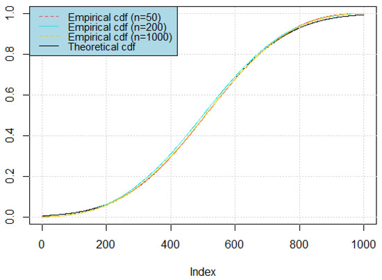
  

  Figure 4. Estimated conditional distribution functions under the quasi-associated AR(1) process for different sample sizes.
  

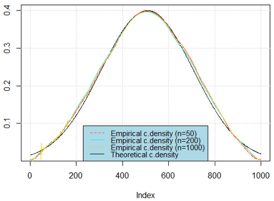  Figure 5. Estimated conditional density functions under the quasi-associated AR(1) process for different sample sizes.
  It is apparent that our estimations exhibit high accuracy when optimal bandwidths are selected. To assess the performance of each model more rigorously, we compute the mean squared error, as shown in Table 1.
  Table 1. MSE of kernel estimators $\widehat{g}$ and $\widehat{G}$ under a quasi-associated AR(1) process ($\rho =0.1$, Binomial$(10,0.25)$ innovations) for sample sizes $n=50,200,1000$.

  Mean Square Error	n = 50	n = 200	n = 1000
  MSE($\widehat{g}$)	$1.11645\times {10}^{-04}$	$8.028238\times {10}^{-05}$	$7.623378\times {10}^{-05}$
  MSE($\widehat{G}$)	$1.017427\times {10}^{-04}$	$3.718499\times {10}^{-05}$	$3.076726\times {10}^{-05}$

  For the next step in achieving the desired objective and firmly establishing the normal approximation of ${\widehat{\lambda }}^s\left(t\right)$ with high effectiveness, we selected the sample that produced an estimate with the smallest MSE (sample size $n=1000$), and followed the subsequent steps:
  • We compute the conditional hazard function estimator using (1), the asymptotic variance $\widehat{{\sigma }_{\widehat{\lambda }}^2}$ defined in (6), and the empirical estimate ${\widehat{\varphi }}_s\left({\theta }_K\right)$.
  • Under the condition:

    $$\underset{n\to \infty }{lim}\sqrt{n{\theta }_H{\varphi }_s\left({\theta }_K\right)}{N}_B^{\lambda }(s,t)=0,$$

    we can ignore the bias term $N_B^{\lambda }(s,t)$ and compute the quantity referred to in (7), namely Quantile Normalized Hazard (QNH), as

    $$\sqrt{{\displaystyle \frac{n{\theta }_H{\widehat{\varphi }}_s\left({\theta }_K\right)}{\widehat{{\sigma }_{\widehat{\lambda }}^2}}}}\left({\widehat{\lambda }}^s\left(t\right)-{\lambda }^s\left(t\right)\right).$$
  • Plot a histogram of QNH and compare it with the standard normal density. (Figure 6).
    

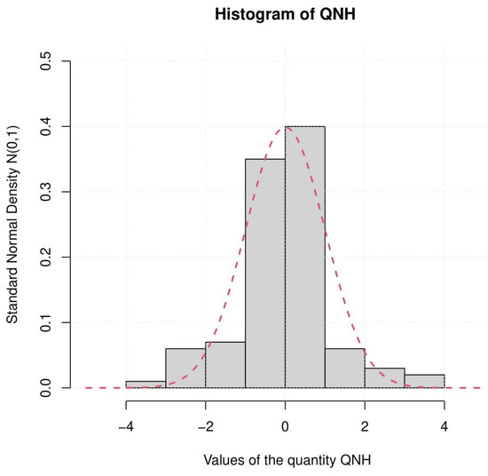    Figure 6. Normal approximation of the conditional hazard function estimator.
  • Finally building a confidence bounds (see Figure 7).
    

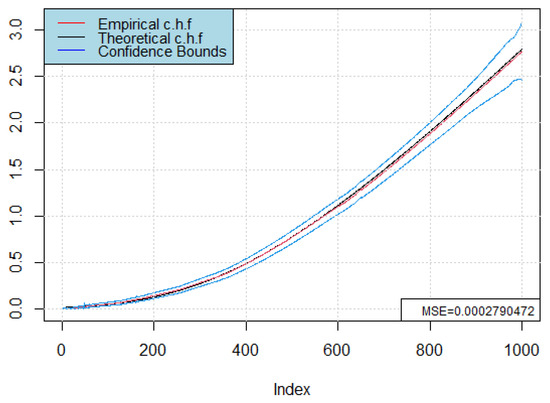    Figure 7. Empirical and theoretical conditional hazard function estimation with confidence bounds.

To complement the graphical evidence and provide a quantitative validation of the asymptotic normality of the QNH statistic, we applied the Kolmogorov–Smirnov (KS) goodness-of-fit test. Specifically, we tested the standardized QNH values against the standard normal distribution for different sample sizes. The results are reported in Table 2.

Table 2. Kolmogorov–Smirnov test results for the QNH statistic under different sample sizes.

Sample Size (n)	KS Statistic	p-Value
50	0.134	0.306
200	0.053	0.604
1000	0.028	0.421

The p-values are all larger than the usual threshold of $0.05$, which means that the null hypothesis of normality cannot be rejected. These results quantitatively confirm that the empirical distribution of the QNH statistic is consistent with the standard normal law, thereby supporting the asymptotic normality established in our main theorem.

5. Conclusions and Some Perspectives

Due to the complexity of the conditional hazard function estimator ${\widehat{\lambda }}^s\left(t\right)$ obtained via the kernel approach, we first decomposed it into three parts, as shown in (A1). The first part corresponds to the numerator of the density estimator, ${\widehat{g}}_N^s\left(t\right)$, which is the dominant component governing the asymptotic properties. We showed that the denominator converges in probability to $1-G^s\left(t\right)$, while the remaining two parts capture the bias arising from ${\widehat{C}}_N^s\left(t\right)$ and ${\widehat{g}}_N^s\left(t\right)$.

From a practical perspective, we conducted a simulation study to validate the theoretical findings. Despite the inherent challenges of bandwidth selection, the proposed estimator exhibited strong performance with low mean squared error. More importantly, the QNH statistic empirically confirmed the asymptotic normality established in the main theorem, thereby demonstrating that the finite-sample results are consistent with the theoretical limit law. These findings highlight both the reliability of the method and its contribution to the broader literature on nonparametric functional estimation.

A potential direction for future work is to examine the sensitivity of the estimator to kernel choice and bandwidth selection procedures. Exploring data-driven or adaptive bandwidth strategies may enhance finite-sample performance. Additionally, investigating the behavior of the estimator in high-dimensional or complex data settings could broaden its practical utility.

This study enhances both the theoretical and empirical comprehension of the asymptotic characteristics of the proposed estimator, laying the foundation for future developments and applications in areas where estimating conditional functional parameters is essential.

References

- Bosq, D.; Lecoutre, J.B. Théorie de L’estimation Fonctionnelle; Economica: Paris, France, 1987. [Google Scholar]
- Ferraty, F.; Vieu, P. Nonparametric Functional Data Analysis: Theory and Practice; Springer Series in Statistics; Springer: Berlin/Heidelberg, Germany, 2006; Available online: https://ideas.repec.org/a/eee/csdana/v51y2007i9p4751-4752.html (accessed on 5 July 2025).
- Ferraty, F.; Mas, A.; Vieu, P. Nonparametric regression on functional data: Inference and practical aspects. Aust. N. Z. J. Stat. 2007, 49, 267–286. [Google Scholar] [CrossRef]
- Lakcasi, A.; Mechab, B. Conditional hazard estimate for functional random fields. J. Stat. Theory Pract. 2014, 8, 192–220. [Google Scholar] [CrossRef]
- Ferraty, F.; Vieu, P. Nonparametric models for functional data, with application in regression, time series prediction and curve discrimination. J. Nonparametric Stat. 2004, 16, 111–125. [Google Scholar] [CrossRef]
- Ferraty, F.; Goia, A.; Vieu, P. Régression non-paramétrique pour des variables aléatoires fonctionnelles mélangeantes. Comptes Rendus Math. 2002, 334, 217–220. [Google Scholar] [CrossRef]
- Mechab, W.; Lakcasi, A. Nonparametric relative regression for associated random variables. Metron 2016, 74, 75–97. [Google Scholar] [CrossRef]
- Azzi, A.; Belguerna, A.; Laksaci, A.; Rachdi, M. The scalar-on-function modal regression for functional time series data. J. Nonparametric Stat. 2023, 36, 503–526. [Google Scholar] [CrossRef]
- Hyndman, R.J.; Yao, Q. Nonparametric estimation and symmetry tests for conditional density functions. J. Nonparametric Stat. 2002, 14, 259–278. [Google Scholar] [CrossRef]
- Attaoui, S.; Laksaci, A.; Ould Said, E. A note on the conditional density estimate in the single functional index model. Stat. Probab. Lett. 2011, 81, 45–53. [Google Scholar] [CrossRef]
- Ling, N.; Xu, Q. Asymptotic normality of conditional density estimation in the single index model for functional time series data. Stat. Probab. Lett. 2012, 82, 2235–2243. [Google Scholar] [CrossRef]
- Abdelhak, K.; Belguerna, A.; Laala, Z. Local Linear Estimator of the Conditional Hazard Function for Index Model in Case of Missing at Random Data. Appl. Appl. Math. Int. J. (AAM) 2022, 17, 33–53. [Google Scholar]
- Daoudi, H.; Mechab, B. Asymptotic Normality of the Kernel Estimate of Conditional Distribution Function for the quasi-associated data. Pak. J. Stat. Oper. Res. 2019, 15, 999–1015. [Google Scholar] [CrossRef]
- Bulinski, A.; Suquet, C. Asymptotical behaviour of some functionals of positively and negatively dependent random fields. Fundam. I Prikl. Mat. 1998, 4, 479–492. [Google Scholar]
- Bouaker, I.; Belguerna, A.; Daoudi, H. The Consistency of the Kernel Estimation of the Function Conditional Density for Quasi-Associated Data in High-Dimensional Statistics. J. Sci. Arts 2022, 22, 247–256. [Google Scholar] [CrossRef]
- Newman, C.M. Asymptotic independence and limit theorems for positively and negatively dependent random variables. Inequalities Stat. Probab. 1984, 5, 127–140. [Google Scholar]
- Ferraty, F.; Rabhi, A.; Vieu, P. Estimation non-paramétrique de la fonction de hasard avec variable explicative fonctionnelle. Rev. Roum. Math. Pures Appl. 2008, 53, 1–18. [Google Scholar]
- Laksaci, A.; Mechab, B. Estimation non-paramétrique de la fonction de hasard avec variable explicative fonctionnelle: Cas des données spatiales. Rev. Roum. Math. Pures Appl. 2010, 55, 35–51. [Google Scholar]
- Gagui, A.; Chouaf, A. On the nonparametric estimation of the conditional hazard estimator in a single functional index. Stat. Transit. New Ser. 2022, 23, 89–105. [Google Scholar] [CrossRef]
- Doukhan, P.; Louhichi, S. A new weak dependence condition and applications to moment inequalities. Stoch. Process. Their Appl. 1999, 84, 313–342. [Google Scholar] [CrossRef]
- Bulinski, A.; Suquet, C. Approximation for quasi-associated random fields. Stat. Probab. Lett. 2001, 54, 215–226. [Google Scholar] [CrossRef]
- Kallabis, R.S.; Neumann, M.H. An exponential inequality under weak dependence. Bernoulli 2006, 12, 333–350. [Google Scholar] [CrossRef]
- Attaoui, S. Sur L’estimation Semi Paramètrique Robuste Pour Statistique Fonctionnelle. Ph.D. Thesis, Université du Littoral Côte d’Opale Lille, France & Université Djillali Liabès, Sidi Bel-Abbès, Algeria, 2012. Available online: https://theses.hal.science/tel-00871026/ (accessed on 2 July 2025).
- Hadjila, T.; Ahmed, A.S. Estimation and simulation of conditional hazard function in the quasi-associated framework when the observations are linked via a functional single-index structure. Commun. Stat.-Theory Methods 2017, 47, 816–838. [Google Scholar] [CrossRef]
- Douge, L. Thèorèmes limites pour des variables quasi-associées hilbertiennes. Ann. L’ISUP 2010, 4, 51–60. [Google Scholar]
- Hamza, D.; Mechab, B.; Zouaoui, C.E. Asymptotic normality of a conditional hazard function estimate in the single index for quasi-associated data. Commun. Stat.-Theory Methods 2020, 49, 513–530. [Google Scholar] [CrossRef]
- Daoudi, H.; Elmezouar, Z.C.; Alshahrani, F. Asymptotic Results of Some Conditional Nonparametric Functional Parameters in High Dimensional Associated Data. Mathematics 2023, 11, 4290. [Google Scholar] [CrossRef]
- Bouzebda, S.; Laksaci, A.; Mohammedi, M. Single Index Regression Model for Functional Quasi-Associated Times Series Data. Revstat-Stat. J. 2023, 20, 605–631. [Google Scholar] [CrossRef]
- Rassoul, A.; Belguerna, A.; Daoudi, H.; Elmezouar, Z.C.; Alshahrani, F. On the Exact Asymptotic Error of the Kernel Estimator of the Conditional Hazard Function for Quasi-Associated Functional Variables. Mathematics 2025, 13, 2172. [Google Scholar] [CrossRef]
- Attaoui, S.; Benouda, O.; Bouzebda, S.; Laksaci, A. Limit theorems for kernel regression estimator for quasi-associated functional censored time series within single index structure. Mathematics 2025, 13, 886. [Google Scholar] [CrossRef]
- Doob, J.L. Stochastic Processes; Wiley: New York, NY, USA, 1953; pp. 228–231. [Google Scholar]
- Chikr-Elmezouar, Z.; Laksaci, A.; Almanjahie, I.M.; Alshahrani, F. Nonparametric Estimation of Dynamic Value-at-Risk: Multifunctional GARCH Model Case. Mathematics 2025, 13, 1961. [Google Scholar] [CrossRef]
- Iglesias-Pérez, M.C. Strong representation of a conditional quantile function estimator with truncated and censored data. Stat. Probab. Lett. 2003, 65, 79–91. [Google Scholar] [CrossRef]
- Yuan, M. GACV for quantile smoothing splines. Comput. Stat. Data Anal. 2006, 50, 813–829. [Google Scholar] [CrossRef]
Disclaimer/Publisher’s Note: The statements, opinions and data contained in all publications are solely those of the individual author(s) and contributor(s) and not of MDPI and/or the editor(s). MDPI and/or the editor(s) disclaim responsibility for any injury to people or property resulting from any ideas, methods, instructions or products referred to in the content. |
© 2025 by the authors. Licensee MDPI, Basel, Switzerland. This article is an open access article distributed under the terms and conditions of the Creative Commons Attribution (CC BY) license (https://creativecommons.org/licenses/by/4.0/).