Larger Size Subspace Codes with Low Communication Overhead

Abstract

Köetter and Kschischang proposed a coding algorithm for network error correction based on subspace codes, which, however, has a high communication overhead (100%). This paper improves upon their coding algorithm and presents a coding algorithm for network error correction with lower communication overhead, which is similar to the communication overhead of classical random network coding. In particular, we utilize the inherent symmetry in subspace codes to optimize the construction process, leading to a more efficient algorithm. At the same time, this paper also studies the construction problem of constant dimension subspace codes, utilizing parallel construction and multilevel construction. By exploiting the symmetry in these methods, we generalize previous results and derive new lower bounds for constant dimension subspace codes.

1. Introduction

Let q be a prime power and ${\mathbb{F}}_q$ be the finite field with q elements which is the field of scalars; the projective space of order n over ${\mathbb{F}}_q$, denoted as ${\mathcal{P}}_q\left(n\right)$, is the set of all subspaces of the vector space ${\mathbb{F}}_q^n$. Projective geometry possesses a natural symmetry, which can influence how subspaces are selected and constructed. Let $k,n$ denote two positive integers with $k\le n$ and let ${\mathcal{G}}_q(n,k)$ be the family of all k-dimensional subspaces in ${\mathbb{F}}_q^n$. For any $\mathcal{U},\mathcal{V}\in {\mathcal{G}}_q(n,k)$, the subspace distance of $\mathcal{U}$ and $\mathcal{V}$ is defined as follows:

$$\begin{array}{ccc}\hfill d_S(\mathcal{U},\mathcal{V})& =& dim(\mathcal{U}+\mathcal{V})-dim(\mathcal{U}\cap \mathcal{V})\hfill \\ & =& dim\left(\mathcal{U}\right)+dim\left(\mathcal{V}\right)-2dim(\mathcal{U}\cap \mathcal{V}).\hfill \end{array}$$

A nonempty subset $\mathcal{C}\subseteq {\mathcal{G}}_q(n,k)$ is called a constant dimension subspace code with parameters ${(n,M,d,k)}_q$, if $\left|\mathcal{C}\right|=M$, and $d_S\left(\mathcal{C}\right)=min\{d_S(\mathcal{U},\mathcal{V}):\mathcal{U},\mathcal{V}\in \mathcal{C},\mathcal{U}\ne \mathcal{V}\}\ge d$.

Constant dimension subspace codes are considered to control errors in random linear network coding which are analogous with the well-known $(n,k)$-code, a k-dimensional subspaces of $F_{q^n}$. As a code, the family of all k-dimensional subspace of ${\mathbb{F}}_{q^n}$ is taken and a code-word is a subspace. The determination of bounds for maximal possible size $A_q(n,d,k)$ of an ${(n,M,d,k)}_q$ constant dimension subspace code is one of the main problems. An online table for lower and upper bounds of $A_q(n,d,k)$ can be found at: https://arxiv.org/abs/1601.02864 (accessed on 1 December 2017) (see [1]).

The rank metric code $\mathcal{M}$ is a subset of the matrix space ${\mathbb{F}}_q^{m\times n}$ endowed with the rank metric $d_R(A,B)=rank(A-B)$. It is well known that the number of codewords in $\mathcal{M}$ is upper bounded by

$$q^{max\{m,n\}\times \left(min\right\{m,n\}-d+1)}$$

(see Refs. [2,3]). A code attaining this bound is referred to as a maximum rank-distance (MRD) code. Lifted MRD codes, parallel construction and multilevel construction are effective techniques for constructing constant dimension subspace codes, with a great deal of results on the construction of constant dimension subspace codes presented in the literature (see [4,5,6,7,8,9,10,11,12,13]).

(1) In [14], Etzion and Silberstein introduced the generalized lifted rank metric codes, referred to as lifted Ferrers diagram rank metric codes. They demonstrated the application of the union of these lifted codes in constructing some constant dimension subspace codes with significantly larger sizes.

(2) In [7], Xianmang He et al. remedied the linkage construction and presented a new construction known as the parallel linkage construction. Many new lower bounds on $A_q(n,d,k)$ were proved from the parallel linkage construction.

(3) In [15], Fagang Li proposed the multilevel linkage construction as an effective improvement on the linkage construction. By combining the multilevel construction and linkage construction, he was able to obtain new lower bounds of constant dimension subspace codes for small parameters.

(4) In [16], Shuangqing Liu et al. introduced a family of new codes called rank metric codes with given ranks, which represent a generalization of both the parallel construction and the classic multilevel construction. Furthermore, many constant dimension subspace codes have been identified with larger size than those of previously best known codes.

In view of the above results, we integrate the parallel and multilevel construction to propose an enhanced version of constant dimension subspace codes in this paper. The aim of this study is to improve the bounds of the previously best known size of the construction for constant dimension subspace codes. In Section 2, we present the essential results that underpin our main results, which are subsequently detailed in Section 3 and Section 4. The sizes of some constant dimension subspace codes are larger than the previously best known bounds in [1]. In Section 5, we offer our concluding remarks.

2. Preliminaries

This section first presents Köetter’s network coding scheme, including the encoding algorithm for the source and the decoding algorithm for the sink. It then introduces some definitions and conclusions related to the construction of constant dimension subspace codes. For more details, please refer to [2,14,17,18].

2.1. Encoding Algorithm for the Source

In the same way as the components of the codewords of traditional Reed–Solomon codes can be obtained by evaluating a regular message polynomial, the basis of the transmission vector space of Köetter and Kschischang [19] is obtained by evaluating a linearized message polynomial. Please refer to Algorithm 1 for specific encoding algorithms. Let ${\mathbb{F}}_q$ be a finite field, and $\mathbb{F}={\mathbb{F}}_{q^m}$ be a finite extension of ${\mathbb{F}}_q$. We can view $\mathbb{F}$ as an m-dimensional vector space over ${\mathbb{F}}_q$.

Firstly, let $A=\{{\alpha }_1,\cdots ,{\alpha }_l\}\subset \mathbb{F}$ be a set of linearly independent elements in the vector space $\mathbb{F}$, then the elements in A span an l-dimensional vector space $⟨A⟩\subseteq \mathbb{F}$ over ${\mathbb{F}}_q$. Using the direct sum, we define an $(l+m)$-dimensional vector space over ${\mathbb{F}}_q$ as follows:

$$W=⟨A⟩\oplus \mathbb{F}=\left\{\right(\alpha ,\beta ):\alpha \in ⟨A⟩,\beta \in \mathbb{F}\}.$$

All the information packets transmitted in the network are vectors in W. Let $P\left(W\right)$ denote all the subspaces of W, and let $P(W,l)$ denote all the subspaces of W with dimension l. The linear space transmitted in the network of this section is the subspace of W generated by the messages U.

Then, let $U=(u_0,u_1,\cdots ,u_{k-1})\in {\mathbb{F}}^k$ be a set of message symbols, which can be viewed as k symbols over $\mathbb{F}$ or as $mk$ symbols over ${\mathbb{F}}_q$. Let $f\left(x\right)={\sum }_{i=0}^{k-1}{u}_i{x}^{q^i}\in {\mathbb{F}}^k\left[x\right]$, where ${\mathbb{F}}^k\left[x\right]$ is the set of linear polynomials of degree at most $q^{k-1}$ over $\mathbb{F}$ and $f\left(x\right)$ is a linear polynomial with the original source message U as its coefficients.

Finally, let ${\beta }_i=f\left({\alpha }_i\right)$, then each pair $({\alpha }_i,{\beta }_i),i=1,\cdots ,l$ can be considered as a vector in W. Since $\{{\alpha }_1,\cdots ,{\alpha }_l\}$ is a linearly independent set, the set $\{({\alpha }_1,{\beta }_1),\cdots ,({\alpha }_l,{\beta }_l)\}$ is also a linearly independent set, and the space generated by this set, denoted as V, is an l-dimensional subspace of W.

Algorithm 1 Encoding steps

1: Input: A set of message symbols u and a linearly independent set $A=\{{\alpha }_1,\cdots ,{\alpha }_l\}$   2: Output: An l-dimensional subspace V in W   3: Define the linear polynomial $f\left(x\right)={\sum }_{i=0}^{k-1}{u}_i{x}^{q^i}\in {\mathbb{F}}^k\left[x\right]$   4: Compute $\beta =\{{\beta }_i=f\left({\alpha }_i\right),i=1,\cdots ,l\}$   5: $V=⟨\left(\begin{array}{cc}{\alpha }_1& {\beta }_1\\ {\alpha }_2& {\beta }_2\\ ⋮& ⋮\\ {\alpha }_l& {\beta }_l\end{array}\right)⟩$

The mapping from the message polynomial $f\left(x\right)={\sum }_{i=0}^{k-1}{u}_i{x}^{q^i}\in {\mathbb{F}}^k\left[x\right]$ to the linear space $V\in P(W,|A\left|\right)$ is denoted as $e{v}_A$. It has been proven in [19] that this mapping is a injective, and the codewords under this mapping form a metric space that satisfies $d\ge 2(l-k+1)$.

Lemma 1

([19]). Let $\mathcal{C}$ be the image set of the mapping $e{v}_A:{\mathbb{F}}^k\left[x\right]\to P(W,|A\left|\right),f\left(x\right)\mapsto V$, where $P(W,|A\left|\right)$ is the set of all $\left|A\right|$-dimensional subspaces in W, and satisfies $l=\left|A\right|\ge k$. Then, $\mathcal{C}$ is a subspace code with parameters $[l+m,l,mk,d=2(l-k+1\left)\right]$.

2.2. Decoding Algorithm for the Sink

Let $V\in \mathcal{C}$ be transmitted over a network, which defines the number of nodes, links, and their connections in this network. Its output is $R=V\oplus E$, where $E\in P\left(W\right)$ is the space spanned by the pollution vector, and ⊕ denotes the sum of spaces. The expression $V\oplus E$ is defined as $\{v+e:v\in V,e\in E\}$, assuming that E and V intersect trivially.

Let the dimension of the space R received by the destination be $r=l+t$, where r is the maximum flow of the network and $\dim (R\cap V)=l$. In this case, $d(R,V)=t$, where t is the dimension of the error space $\dim \left(E\right)=t$. From the proof in [19], it is known that when the received space $R=V\oplus E$ and $2t<d$, the minimum distance decoding for C can retrieve the space V, thereby obtaining the original source message U.

Lemma 2

([19]). The communication overhead of the network error-correcting coding system by Kötter is 100%.

2.3. Constant Dimension Subspace Codes

For a constant dimension subspace code $\mathcal{C}\subseteq {\mathcal{G}}_q(n,k)$, each codeword U of $\mathcal{C}$ can be represented by a $k\times n$ generator matrix whose k rows form a basis for U. The Gaussian elimination algorithm gives a unique generator matrix in reduced row echelon form denoted by $E\left(U\right)$. A binary row vector $v\left(U\right)$ of length n and weight k is called the identifying vector of U, where the k ones of $v\left(U\right)$ are exactly the pivots of $E\left(U\right)$. The Ferrers tableau of U, denoted by $\mathcal{F}\left(U\right)$, is acquired by removing the columns which contain the pivots of $E\left(X\right)$ and the zeroes from each row of $E\left(X\right)$ to the left of the pivots. The Ferrers diagram ${\mathcal{F}}_U$ of U, which only depends on the identifying vector $v\left(U\right)$, arises from $\mathcal{F}\left(U\right)$ by replacing the entries of $\mathcal{F}\left(U\right)$ with dots.

Example 1.

Let U be a $three$-dimensional subspace of ${\mathcal{G}}_2(8,3)$ with the following generator matrix in reduced row echelon form:

$$E\left(U\right)=\left(\begin{array}{cccccccc}1& 0& 0& 0& 0& 1& 0& 0\\ 0& 0& 1& 0& 1& 0& 0& 1\\ 0& 0& 0& 1& 1& 0& 0& 0\end{array}\right).$$

Then, the identifying vector of U is $v\left(U\right)=\left(10110000\right)$ and the corresponding Ferrers tableaus $\mathcal{F}\left(U\right)$ is

$$\begin{array}{ccccc}0& 0& 1& 0& 0\\ & 1& 0& 0& 1\\ & 1& 0& 0& 0\end{array},$$

and the corresponding Ferrers diagram ${\mathcal{F}}_U$ of U is

$$\begin{array}{ccccc}•& •& •& •& •\\ & •& •& •& •\\ & •& •& •& •\end{array}.$$

Let $\mathcal{F}$ be a $k\times n$ Ferrers diagram. A linear rank metric code ${\mathcal{C}}_{\mathcal{F}}\subseteq {\mathbb{F}}_q^{k\times n}$ is called a $Ferrers$ $diagram$ $rank$ $metric$ $code$ if every matrix $M\in {\mathcal{C}}_{\mathcal{F}}$ has shape $\mathcal{F}$, that is, all entries of M not in $\mathcal{F}$ are zeroes. A Ferrers diagram rank metric code is called an $[\mathcal{F},\rho ,d]$-code if rank$\left(M\right)\ge d$ for an arbitrary nonzero codeword $M\in {\mathcal{C}}_{\mathcal{F}}$ and dim$\left({\mathcal{C}}_{\mathcal{F}}\right)=\rho$.

2.4. Related Works

T. Etzion et al. [14] show that the Hamming distance can be applied to the lower bound of the subspace distance. It plays an important role in obtaining the desired subspace distance. The specific instructions are as follows. For any $U,V\in {\mathcal{G}}_q(n,k)$, then

$$d_S(U,V)\ge d_H(v\left(U\right),v\left(V\right)),$$

(1)

where $d_H(v\left(U\right),v\left(V\right))$ denotes the Hamming distance between $v\left(U\right)$ and $v\left(V\right)$.

Lemma 3.

Let ${\mathcal{C}}_{\mathcal{F}}\subseteq {\mathbb{F}}_q^{k\times n}$ be an $[\mathcal{F},\rho ,d]$-code. Then, the upper bound of the cardinality of ${\mathcal{C}}_{\mathcal{F}}$ is $q^{mi{n}_i\left\{t_i\right\}}$, where $t_i$ is the number of dots in $\mathcal{F}$, which are neither contained in the first i rows nor contained in the last $d-1-i$ columns for $0\le i\le d-1$.

An $[\mathcal{F},\rho ,d]$-code is called an $optimal$ $Ferrers$ $diagram$ $rank$ $metric$ $code$ if it attains the upper bound of $q^{mi{n}_i\left\{t_i\right\}}$. The existence of an optimal Ferrers diagram rank metric code has been proven but is still considered as widely open (see [17,20,21,22]). The following lemma is a criterion for checking the existence of an optimal Ferrers diagram rank metric code.

Lemma 4.

Let $\mathcal{F}$ be a $k\times n$ $(k\ge n)$ Ferrers diagram and ${ϵ}_i$ be the number of dots in the i-th column of $\mathcal{F}$. If each of the rightmost $d-1$ columns of $\mathcal{F}$ has at least n dots, then there exists an optimal $[\mathcal{F},{\sum }_{i=1}^{n-d+1}{ϵ}_i,d]$ code for any prime power q.

For a Ferrers diagram $\mathcal{F}$ of size $k\ge n$, one can transpose it to obtain a Ferrers diagram ${\mathcal{F}}^T$ of size $n\ge k$, where the rightmost column of $\mathcal{F}$ is the first row of ${\mathcal{F}}^T$ and so on. Thus, if there exists an optimal Ferrers diagram rank metric code for $\mathcal{F}$, then so does an optimal Ferrers diagram rank metric code for ${\mathcal{F}}^T$.

T. Etzion et al. [14] also provided the relevant theorem for a lifted constant dimension subspace code.

Lemma 5.

Let ${\mathcal{C}}_{\mathcal{F}}\subseteq {\mathbb{F}}_q^{k\times (n-k)}$ be an $[\mathcal{F},\rho ,d]$ Ferrers diagram rank metric code. Then, the lifted constant dimension subspace code ${\tilde{\mathcal{C}}}_{\mathcal{F}}$ defined by

$${\tilde{\mathcal{C}}}_{\mathcal{F}}=\{U\in {\mathcal{G}}_q(n,k):\mathcal{F}\left(U\right)\in {\mathcal{C}}_{\mathcal{F}},{\mathcal{F}}_U=\mathcal{F}\}$$

(2)

is an ${(n,q^{\rho },2d,k)}_q$ constant dimension subspace code.

Lemma 6.

Let Λ be an index set and $S=\{v_i\in {\mathbb{F}}_2^n:w_H\left(v_i\right)=k,i\in \Lambda \}$ be the set of identifying vectors with $d_H\left(S\right)=min\{d_H(v_i,v_j):i\in \Lambda \}=2d$, where $w_H(·)$ is the Hamming weight. For each $v\in S$, let ${\mathcal{C}}_v\subseteq {\mathcal{G}}_q(n,k)$ be an $(n,|{\mathcal{C}}_v{|,2d,k)}_q$ constant dimension subspace code; then, $\mathcal{C}={\cup }_{v\in S}{\mathcal{C}}_v$ is an ${(n,|\mathcal{C}|,2d,k)}_q$ constant dimension subspace code with cardinality ${\sum }_{v\in S}\left|{\mathcal{C}}_v\right|.$

Lemma 7.

For a matrix $M\in {\mathbb{F}}_q^{k\times n}$, the row space of M over ${\mathbb{F}}_q$ is denoted by $rs\left(M\right)$. A set $\mathcal{M}\subseteq {\mathbb{F}}_q^{k\times n}$ of $k\times n$ matrices over ${\mathbb{F}}_q$ is called an $SC$-$representation$ of a constant dimension subspace code in ${\mathcal{G}}_q(n,k)$ if the following conditions are satisfied.

(a) 

For each $M\in \mathcal{M}$, $rank\left(M\right)=k$.

(b) 

For any two distinct matrices $M_1,M_2\in \mathcal{M},rs\left(M_1\right)\ne rs\left(M_2\right)$, where $rs\left(M_1\right)$ is an ${\mathbb{F}}_q$-subspace of ${\mathbb{F}}_q^n$ generalized by all row vectors of $M_1$.

X. He et al. [7] remedied the linkage construction and presented a new construction known as the parallel linkage construction. Many new lower bounds on $A_q(n,d,k)$ were proved from the parallel linkage construction.

Lemma 8.

Let $\mathcal{U}$ and $\mathcal{V}$ be SC-representations of two, ${(m,N_1,2d,k)}_q$ and ${(n,N_2,2d,k)}_q$, constant dimension subspace codes, respectively. Let $\mathcal{P}\subseteq {\mathbb{F}}_q^{k\times n}$ be a code with rank distance d and $N_3$ elements. Let $\mathcal{Q}\subseteq {\mathbb{F}}_q^{k\times m}$ be a code with rank distance d and $N_4$ elements such that the rank of each element in $\mathcal{Q}$ is at most $k-d$. Consider the set defined by $\mathcal{C}={\mathcal{C}}_1\cup {\mathcal{C}}_2$, where

$${\mathcal{C}}_1=\{rs\left(U\right|P):U\in \mathcal{U},P\in \mathcal{P}\},$$

(3)

$${\mathcal{C}}_2=\{rs\left(Q\right|V):Q\in \mathcal{Q},V\in \mathcal{V}\}.$$

(4)

Then, $\mathcal{C}$ is an ${(m+n,N_1{N}_3+N_2{N}_4,2d,k)}_q$ constant dimension subspace code.

F. Li [15] proposed the multilevel linkage construction as an effective improvement on the linkage construction.

Lemma 9.

Let $m,n,k,d$ be integers with $m,n\ge k$ and $k\ge 2d$. Let $\mathcal{U}$ and $\mathcal{V}$ be SC-representations of two, ${(m,N_1,2d,k)}_q$ and ${(n,N_2,2d,k)}_q$, constant dimension subspace codes, respectively. Let $\mathcal{P}\subseteq {\mathbb{F}}_q^{k\times n}$ be a code with rank distance d and $N_3$ elements. Let Λ be an index set and $S=\{v_i\in {\mathbb{F}}_2^{m+n}:w_H\left(v_i\right)=k,i\in \Lambda \}$ be the set of identifying vectors with $d_H\left(S\right)=2d$ such that the Hamming weight of each $v_i=(v_i^1,v_i^2)\in S$ satisfy $w_H\left(v_i^1\right),w_H\left(v_i^2\right)\ge d$, where $v_i^1\in {\mathbb{F}}_2^m$ and $v_i^2\in {\mathbb{F}}_2^n$. Let ${\mathcal{C}}_{v_i}\subseteq {\mathbb{F}}_q^{k\times (m+n-k)}$ be a Ferrers diagram rank metric code with $d_R\left({\mathcal{C}}_{v_i}\right)=d$. Consider the constant dimension subspace code defined by

$$\mathcal{C}={\mathcal{C}}_1\cup {\mathcal{C}}_2\cup \left({\cup }_{v_i\in S}{\tilde{\mathcal{C}}}_{v_i}\right),$$

where ${\mathcal{C}}_1$ is the same as Equation (3), ${\mathcal{C}}_2=\{rs\left(0_{k\times m}\right|V):V\in \mathcal{V}\}$, and ${\tilde{\mathcal{C}}}_{v_i}$ is the lifted code of ${\mathcal{C}}_{v_i}$. Then, $\mathcal{C}$ is an ${(m+n,|\mathcal{C}|,2d,k)}_q$ constant dimension subspace code with $\left|\mathcal{C}\right|=N_1{N}_3+N_2+{\sum }_{v_i\in S}\left|{\mathcal{C}}_{v_i}\right|$.

Let $\mathcal{M}\subseteq {\mathbb{F}}_q^{k\times n}$; the $rankdistribution$ of $\mathcal{M}$ is defined by

$$A_i\left(\mathcal{M}\right)=\left|\{M\in \mathcal{M}:rank\left(M\right)=i\}\right|.$$

The rank distribution of an MRD code is completely determined by its parameters. The following results can be referred to in Corollary 26 in [18] or Theorem 5.6 in [2]. The Delsarte Theorem is essential to calculating the final result in this paper.

Lemma 10.

Let $\mathcal{M}\subseteq {\mathbb{F}}_q^{k\times n}(n\ge k)$ be an MRD code with rank distance d; then, its rank distribution is given by

$$A_r\left(\mathcal{M}\right)={\left({\displaystyle \genfrac{}{}{0pt}{}{k}{r}}\right)}_q\sum _{i=0}^{r-d}{(-1)}^i{q}^{\left({\displaystyle \genfrac{}{}{0pt}{}{i}{2}}\right)}{\left({\displaystyle \genfrac{}{}{0pt}{}{r}{i}}\right)}_q({\displaystyle \frac{q^{n(k-d+1)}}{q^{n(k+i-r)}}}-1).$$

3. Subspace Codes with Low Communication Overhead

In this section, we assume that the source and the destination share a public random number generator. Let ${\mathbb{F}}_q$ be a finite field, and let $\mathbb{F}={\mathbb{F}}_{q^m}$ and ${\mathbb{F}}_{q^l}$ be finite extensions of ${\mathbb{F}}_q$, satisfying $l|m$, i.e., ${\mathbb{F}}_{q^l}\subseteq \mathbb{F}$. We can view $\mathbb{F}$ and ${\mathbb{F}}_{q^l}$ as m-dimensional and l-dimensional vector spaces over ${\mathbb{F}}_q$, respectively.

As a preparatory step for the source coding algorithm, the source first selects a set of linearly independent vectors $g_1,\cdots ,g_l$ in the finite field ${\mathbb{F}}_q$.

Let

$$G=\left(\begin{array}{cccc}{g}_{11}& g_{12}& \cdots & g_{1l}\\ g_{21}& g_{22}& \cdots & g_{2l}\\ ⋮& ⋮& \ddots & ⋮\\ g_{l1}& g_{l2}& \cdots & g_{ll}\end{array}\right)=\left(\begin{array}{c}{g}_1\\ g_2\\ ⋮\\ g_l\end{array}\right).$$

The vector space $(g_1,\cdots ,g_l)$ that spans over ${\mathbb{F}}_q$ is given by $⟨G⟩={\mathbb{F}}_q^l$, where G is the set of vectors composed of $(g_1,\dots ,g_l)$. It is obvious that $⟨G⟩$ is the entire space ${\mathbb{F}}_q^l$. We define an $(l+m)$-dimensional vector space over ${\mathbb{F}}_q$ using the direct sum:

$$W=⟨G⟩\oplus \mathbb{F}=\left\{\right(\alpha ,\beta ):\alpha \in ⟨G⟩,\beta \in \mathbb{F}\}.$$

All the information packets transmitted in the network are vectors in W. Let $P\left(W\right)$ denote all the subspaces of W, and let $P(W,l)$ denote all the subspaces of W with dimension l. The linear space transmitted in the network of this section is the subspace of W generated by the messages U.

3.1. Encoding Algorithm for the Source

The source generates a vector space $V\in P(W,l)$ from the original source message U through the following steps:

Step 1: First, select a permutation matrix P of size $n\times n$ over the finite field ${\mathbb{F}}_q$.

Step 2: Generate the matrix A as follows:

$$A=\left(E_l\right|O_{l\times (n-l)})P=\left(\begin{array}{cccc}{a}_{11}& a_{12}& \cdots & a_{1m}\\ a_{21}& a_{22}& \cdots & a_{2m}\\ ⋮& ⋮& \ddots & ⋮\\ a_{l1}& a_{l2}& \cdots & a_{lm}\end{array}\right)=\left(\begin{array}{c}{a}_1\\ a_2\\ ⋮\\ a_l\end{array}\right),$$

where $E_l$ is is the unit matrix of order l, and $O_{l\times (n-l)}$ is the zero matrix with size $l\times (n-l)$. Obviously, $a_1,\dots ,a_l$ must be a set of linearly independent vectors.

Step 3: Generate a set of vectors $d_1,\dots ,d_l$ with length m from matrices G and A as follows:

$$D=\left(\begin{array}{c}{d}_1\\ d_2\\ ⋮\\ d_l\end{array}\right)=GA=\left(\begin{array}{cccc}{g}_{11}& g_{12}& \cdots & g_{1l}\\ g_{21}& g_{22}& \cdots & g_{2l}\\ ⋮& ⋮& \ddots & ⋮\\ g_{l1}& g_{l2}& \cdots & g_{ll}\end{array}\right)\left(\begin{array}{cccc}{a}_{11}& a_{12}& \cdots & a_{1m}\\ a_{21}& a_{22}& \cdots & a_{2m}\\ ⋮& ⋮& \ddots & ⋮\\ a_{l1}& a_{l2}& \cdots & a_{lm}\end{array}\right).$$

Let the mapping from $g_i$ to $d_i$ be denoted as $\varphi :g\left(z\right)=zA$; then, this mapping is injective.

Step 4: Let $f\left(x\right)={\sum }_{i=0}^{k-1}{u}_i{x}^{q^i}\in {\mathbb{F}}^k\left[x\right]$ be a linear polynomial with the original source message $U=(u_0,u_1,\cdots ,u_{k-1})\in {\mathbb{F}}^k$ as its coefficient.

Step 5: Let ${\beta }_i=f\left(d_i\right)={\sum }_{i=0}^{k-1}{u}_i{d}^{q^i}$; then, each pair $(g_i,{\beta }_i),i=1,\cdots ,l$ can be considered as a vector in W. The set $\{(g_1,{\beta }_1),\cdots ,(g_l,{\beta }_l)\}$ is a linearly independent set, and the space generated by this set, denoted as V, is a subspace of dimensions l of W. The space V is the vector space that the source ultimately needs to transmit over the network.

Let the mapping from $d_1,\dots ,d_l$ to the linear space $V\in P(W,|A\left|\right)$ be denoted as $\psi :f\left(x\right)={\sum }_{i=0}^{k-1}{u}_i{x}^{q^i}$. Let $e{v}_A$ be a new mapping defined by the functions $\varphi$ and $\psi$ that map the original source message $U=(u_0,u_1,\cdots ,u_{k-1})$ to the vector space $V\in P(W,|A\left|\right)$. Obviously, the mapping $e{v}_A$ can be constructed by the function $H\left(z\right)=f\left(g\right(z\left)\right)$, where $f\left(x\right)\in {\mathbb{F}}^k\left[x\right]$ and z is a vector of length l over ${\mathbb{F}}_q$.

The following is a case study that analyzes the specific process of subspace codes in network transmission through a designed network. Let $q=2$, $m=4$, $k=2$, and $l=3$. The finite field $\mathbb{F}={\mathbb{F}}_2^4$ is generated by the fourth-degree polynomial $g\left(x\right)=x^4+x^3+1$ over ${\mathbb{F}}_2$. Let $u=(9,14)\in {\mathbb{F}}^2$ be a set of information symbols containing two symbols in ${\mathbb{F}}_2$. The analysis is conducted in two aspects: encoding steps and transmission steps.

3.1.1. Encoding Steps

• Let the linear polynomial corresponding to the information symbols $u=(9,14)$ be $f\left(x\right)=9x+14x^2$.
• Let $G=\{1,\alpha ,{\alpha }^2\}=\{1,2,4\}$ be a linearly independent set of elements in the vector space $\mathbb{F}$ with the appropriate matrix $A=\left(E_l\right|O_{l\times (n-l)})$; then, $D=\{1,2,4\}$.
• $\beta =\{{\beta }_i=f\left(d_i\right)\}=\{7,10,4\}$.

Thus, the linear space V is given as follows: $V=⟨\left(\begin{array}{cc}1& 7\\ 2& 10\\ 4& 4\end{array}\right)⟩.$

The elements in V are expanded over ${\mathbb{F}}_2$, with the least significant bit placed in the leftmost position. For example, $1=100$, $4=001$, $7=1110$, etc. Therefore, the subspace codeword actually transmitted is as follows: $V=⟨\left(\begin{array}{cc}100& 1110\\ 010& 0101\\ 001& 0010\end{array}\right)⟩.$

3.1.2. Transmission Steps

A communication network is set up as shown in Figure 1. Assume that any node in the network can perform network coding and that the error probability on each network link is 0. The encoder-generated codeword is a subspace, and in fact, only the row vectors of the generator matrix of this codeword are transmitted. Each row of the generator matrix is treated as a packet and the source transmits one packet on each outgoing link. The transmitted codeword V contains three packets: $p_1=\left(1001110\right),p_2=\left(0100101\right),p_3=\left(0010010\right)$.

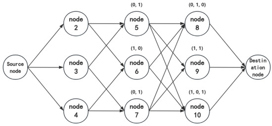
Figure 1. Communication network.

Now let us analyze how packets are transmitted in the network and received by the sink. Assume that transmission occurs one bit at a time.

Step 1: The source sends the packets $p_1$, $p_2$, and $p_3$ to intermediate nodes 2, 3, and 4, respectively.

Step 2: Node 2 forwards the received packet $p_1$ to nodes 5 and 6; node 3 forwards the received packet $p_2$ to nodes 5 and 7; and node 4 forwards the received packet $p_3$ to nodes 6 and 7.

Step 3: The local encoding kernels for nodes 5, 6, and 7 are $(0,1)$, $(1,0)$, and $(0,1)$, respectively. Therefore, node 5 will receive the packets $p_1$ and $p_2$ and, after encoding, obtain the new packet $p_5=(p_1,p_2)·{(0,1)}^T=p_2$, which it sends to nodes 8, 9, and 10. Node 6 will obtain $p_6=(p_1,p_3)·{(1,0)}^T=p_1$ and send it to nodes 8 and 10. Node 7 will obtain $p_7=(p_2,p_3)·{(0,1)}^T=p_3$ and send it to nodes 8, 9, and 10.

Step 4: The local encoding kernels for nodes 8, 9, and 10 are $(0,1,0)$, $(1,1)$, and $(1,0,1)$, respectively. Thus, node 8 will obtain $p_8=(p_2,p_1,p_3)·{(0,1,0)}^T=p_1$ and send it to the sink node; node 9 will obtain $p_9=(p_2,p_3)·{(1,1)}^T=p_2+p_3$ and send it to the sink node; and node 10 will obtain $p_{10}=(p_2,p_1,p_3)·{(1,0,1)}^T=p_2+p_3$ and send it to the sink node. The three packets received by the sink node form the following matrix: $M=\left(\begin{array}{cc}100& 1110\\ 011& 0111\\ 011& 0111\end{array}\right).$

The matrix M formed by the packets received at the sink represents the generating matrix of the received codeword U, where $U=⟨M⟩$. The basis of the received codeword U can be directly found as $\left\{\right(1001110),(0110111\left)\right\}$. Using the decoding algorithm, we can recover the original information $u=(9,14)$.

Lemma 11.

The mapping $\varphi :g\left(z\right)=zA$ is injective.

Proof. 

Using proof by contradiction, assume there exists another vector y of length l, where $y=(y_1,\cdots ,y_l)$ and $z=(z_1,\cdots ,z_l)\in {\mathbb{F}}_q$, such that $yA=zA$. Then, we have

$$y_1{a}_1+\cdots +y_l{a}_l=z_1{a}_1+\cdots +z_l{a}_l.$$

The above equation can be converted into $(y_1-z_1)a_1+\cdots +(y_l-z_l)a_l=0.$ Since $a_1,\dots ,a_l$ is a set of linearly independent vectors, the above equation holds if and only if $y_i=z_i$ for $i=1,\cdots ,l$.  □

Lemma 12.

Let $l\ge k$, then the mapping $e{v}_A:H\left(z\right)=f\left(g\left(z\right)\right)$ is injective.

Proof. 

Since we have already proven that the mapping $\varphi :g\left(z\right)=zA$ is injective, we only need to show that the mapping $\psi$ is also injective.

Using proof by contradiction, assume there exists another linear polynomial $h\left(x\right)$, $f\left(x\right),h\left(x\right)\in {\mathbb{F}}^K\left[X\right]$ such that $H^{\prime }\left(g_i\right)=h\left(g\left(g_i\right)\right)={\beta }_i,i=1,\cdots ,k$. Let $K\left(z\right)=H\left(z\right)-H^{\prime }\left(z\right)=f\left(g\left(z\right)\right)-h\left(g\left(z\right)\right)$. Clearly, $K\left(g_i\right)=0$ for $i=1,\cdots ,k$. Since $g_1,\cdots ,g_l$ are linearly independent and $K\left(z\right)$ is a polynomial of a degree less than $k-1$, the assumption holds if and only if $K\left(z\right)\equiv 0$, that is, $f\left(x\right)\equiv h\left(x\right)$.  □

Lemma 13.

Let $\{(g_1,{\beta }_1),\cdots ,(g_l,{\beta }_l)\}\subseteq W$ be a set of r linearly independent vectors that satisfy ${\beta }_i=H\left(g_i\right)$, where $H\left(z\right)=f\left(g\right(z\left)\right)$. Then, $(g_1,\cdots ,g_l)$ are also linearly independent.

Proof. 

Using proof by contradiction, assume there exists a set of coefficients ${\gamma }_1,\cdots ,{\gamma }_r\in {\mathbb{F}}_q$ such that ${\sum }_{i=1}^r{\gamma }_i{g}_i=0$. The above equation can be rearranged as follows:

$$\sum _{i=1}^r{\gamma }_i(g_i,{\beta }_i)=(\sum _{i=1}^r{\gamma }_i{g}_i,\sum _{i=1}^r{\gamma }_{i}H(g_i))=(0,H(\sum _{i=1}^r{\gamma }_i{g}_i))=(0,0).$$

Given that $(g_1,{\beta }_1),\cdots ,(g_r,{\beta }_r)$ are linearly independent, the assumption holds if and only if ${\gamma }_1,\cdots ,{\gamma }_r=0$.  □

Theorem 1.

Let C be the message space obtained from the mapping $e{v}_A$ that satisfies $l\ge k$. Then, under the subspace metric, it holds that $d\ge 2(l-k+1)$.

Proof. 

Assume $f_1\left(x\right)$ and $f_2\left(x\right)$ are two distinct linear polynomials in ${\mathbb{F}}^k\left[x\right]$ such that $f(g\left(z\right))=H_1\left(z\right)=H_2\left(z\right)=f_2\left(g\left(z\right)\right)$. The corresponding vector spaces under the mapping $e{v}_A$ are $V_1=e{v}_A\left(H_1\right)$ and $V_2=e{v}_A\left(H_2\right)$. Assume the dimension of the space $V_1\cap V_2$ is r, meaning there exist r linearly independent vectors $(g_1^{\prime },{\beta }_1^{\prime }),\cdots ,(g_r^{\prime },{\beta }_r^{\prime })$ in $V_1\cap V_2$, such that $H_1\left(g_i^{\prime }\right)=H_2\left(g_i^{\prime }\right)={\beta }_i^{\prime },i=1,\cdots ,r.$ By Lemma 13, $(g_1^{\prime },\cdots ,g_r^{\prime })$ is also a set of linearly independent vectors, thus they span an r-dimensional linear space, denoted as B. In the space B, all vectors $b\in B$ satisfy $H_1\left(b\right)=H_2\left(b\right)=0$. If $r\ge k$, then the polynomials $H_1\left(z\right)$ and $H_2\left(z\right)$ would have more than k common roots, and since they are both polynomials of a degree less than k, then we have $H_1\left(z\right)\equiv H_2\left(z\right)$, which contradicts our assumption. Therefore, $r<k-1$, leading to

$$d(V_1,V_2)=dim\left(V_1\right)+dim\left(V_2\right)-2dim(V_1\cap V_2)=2(l-r)>2(l-m+1).$$

□

3.2. Decoding Algorithm for the Sink

Let the vector space received by the destination be $R=V\oplus E$, where $E\in P\left(W\right)$ is the space spanned by the pollution vector, and ⊕ denotes the sum of spaces. The expression $V\oplus E$ is defined as $\{v+e:v\in V,e\in E\}$, where E and V intersect trivially. Let the dimension of the space R received by the destination be $r=l+t$, where r is the maximum flow of the network and $\dim (R\cap V)=l$. In this case, $d(R,V)=t$, where t is the dimension of the error space $\dim \left(E\right)=t$.

The following theorem is a special case of Theorem 2 in [19].

Theorem 2.

Let C be the set of vector spaces to be transmitted, and let $V\in C$ be the vector space to be transmitted. Let $R=V\oplus E$ be the vector space received by the receiver, where $\mathit{dim}\left(E\right)=t$. If $2t<d\left(C\right)$, then the minimum distance decoding on C can recover the original source message U from the received vector space R.

Proof. 

For the space C, we have $d(V,R)\le t$. Assume $T\ne V$ is another vector space in C. Then, we have $d(V,T)\le d(V,R)+d(R,T)$, which implies $d(R,T)\ge d\left(C\right)-d(V,R)\ge d\left(C\right)-t.$ If $2t<d\left(C\right)$ holds, then $d(R,T)>d(R,V)$, meaning that minimum distance decoding can recover the space V.

Given the vector space V, let $(g_1^{\prime },{\beta }_1^{\prime }),\cdots ,(g_l^{\prime },{\beta }_l^{\prime })$ be a basis for the space V. Then, we have ${\beta }_i^{\prime }=H\left(g_i^{\prime }\right)=f\left(g\left(g_i^{\prime }\right)\right)i=1,2,\cdots ,l.$ The receiver selects the first k equations ${\beta }_i^{\prime }=H\left(g_i^{\prime }\right)$, where $i=1,2,\cdots ,k$, and rewrites them as follows:

$$(u_0,\cdots ,u_{k-1})\left(\begin{array}{cccc}{a}_1^{\prime }& a_2^{\prime }& \cdots & a_k^{\prime }\\ a_1^{\prime q}& a_2^{\prime q}& \cdots & a_k^{\prime q}\\ ⋮& ⋮& \ddots & ⋮\\ a_1^{\prime q^{k-1}}& a_2^{\prime q^{k-1}}& \cdots & a_k^{\prime q^{k-1}}\end{array}\right)=({\beta }_1,\cdots ,{\beta }_k),$$

where

$$A^{\prime }=\left(\begin{array}{c}{a}_1^{\prime }\\ a_2^{\prime }\\ ⋮\\ a_k^{\prime }\end{array}\right)=G^{\prime }A=\left(\begin{array}{cccc}{g}_{11}^{\prime }& g_{12}^{\prime }& \cdots & g_{1l}^{\prime }\\ g_{21}^{\prime }& g_{22}^{\prime }& \cdots & g_{2l}^{\prime }\\ ⋮& ⋮& \ddots & ⋮\\ g_{k1}^{\prime }& g_{k2}^{\prime }& \cdots & g_{kl}^{\prime }\end{array}\right)\left(\begin{array}{cccc}{a}_{11}& a_{12}& \cdots & a_{1m}\\ a_{21}& a_{22}& \cdots & a_{2m}\\ ⋮& ⋮& \ddots & ⋮\\ a_{l1}& a_{l2}& \cdots & a_{lm}\end{array}\right).$$

Then, the original source message U can be solved as follows:

$$(u_0,\cdots ,u_{k-1})=({\beta }_1^{\prime },\cdots ,{\beta }_k^{\prime }){\left(\begin{array}{cccc}{a}_1^{\prime }& a_2^{\prime }& \cdots & a_k^{\prime }\\ a_1^{\prime q}& a_2^{\prime q}& \cdots & a_k^{\prime q}\\ ⋮& ⋮& \ddots & ⋮\\ a_1^{\prime q^{k-1}}& a_2^{\prime q^{k-1}}& \cdots & a_k^{\prime q^{k-1}}\end{array}\right)}^{-1}.$$

□

Corollary 1.

The communication overhead of the above network error correction coding system is ${\displaystyle \frac{k}{m}}$.

Proof. 

In the source encoding algorithm, the communication overhead introduced by the $k\times k$ matrix G is given by ${\displaystyle \frac{k}{m}}$. The matrix G can completely be an $m\times m$ identity matrix. □

4. Subspace Codes with Larger Size

In this section, we combine the parallel construction and multilevel construction to propose an improved version. As a consequence, we improve the bounds of the previously best known construction for constant dimension subspace codes in [1].

Theorem 3.

Let $m,n,k$ be integers with $m,n\ge k$ and Λ be an index set. Let

$$S=\{v_i=(v_i^1,0_n)\in {\mathbb{F}}_2^{m+n}:v_i^1\in {\mathbb{F}}_2^m,w_H\left(v_i^1\right)=k,i\in \Lambda \}$$

be the set of identifying vectors with $d_H\left(S\right)=2d$, where $0_n$ is the zero vector with length n. Let ${\mathcal{C}}_{v_i}\subseteq {\mathbb{F}}_q^{k\times (m+n-k)}$ be a Ferrers diagram rank metric code with $d_R\left({\mathcal{C}}_{v_i}\right)=d$ and ${\tilde{\mathcal{C}}}_{v_i}$ be the lifted code of ${\mathcal{C}}_{v_i}$. Consider the constant dimension subspace code defined by

$$\mathcal{C}=\left({\cup }_{v_i\in S}{\tilde{\mathcal{C}}}_{v_i}\right)\cup {\mathcal{C}}_2,$$

where ${\mathcal{C}}_2$ is the same as in Equation (4). Then, $\mathcal{C}$ is an ${(m+n,|\mathcal{C}|,2d,k)}_q$ constant dimension subspace code with $\left|\mathcal{C}\right|={\sum }_{v_i\in S}\left|{\mathcal{C}}_{v_i}\right|+N_2{N}_4$.

Proof. 

It is clear that ${\tilde{\mathcal{C}}}_{v_i}$ and ${\mathcal{C}}_2$, $v_i\in S$, are pairwise disjoint. According to Equation (4) and the definition of $\mathcal{C}$, it is easy to verify that

$$\left|\mathcal{C}\right|=\sum _{v_i\in S}\left|{\mathcal{C}}_{v_i}\right|+N_2{N}_4.$$

Now we determine the minimum distance of $\mathcal{C}$ in the following four cases.

Case 1: Let $\mathcal{X}$ and ${\mathcal{X}}^{\prime }$ be two subspaces in ${\tilde{\mathcal{C}}}_{v_i}$, $v_i\in S.$ Since $d_R\left({\mathcal{C}}_{v_i}\right)=d$ and Equation (2), $d_S(\mathcal{X},{\mathcal{X}}^{\prime })\ge d_S\left({\tilde{\mathcal{C}}}_{v_i}\right)=2d.$

Case 2: For two distinct vectors $v_i$ and $v_j$ in S, let ${\mathcal{X}}_i\in {\tilde{\mathcal{C}}}_{v_i}$ and ${\mathcal{X}}_j\in {\tilde{\mathcal{C}}}_{v_j}$. By Equation (1), $d_S({\mathcal{X}}_i,{\mathcal{X}}_j)\ge d_H(v_i,v_j)\ge d_H\left(S\right)=2d.$

Case 3: Let $\mathcal{Y}$ and ${\mathcal{Y}}^{\prime }$ be two subspaces in ${\mathcal{C}}_2$. Then,

$$\mathcal{Y}\cap {\mathcal{Y}}^{\prime }=\{x\left(Q\right|V)=y\left(Q^{\prime }\right|V^{\prime }):x,y\in {\mathbb{F}}_q^k\}.$$

• If $V\ne V^{\prime }$, it is easy to check that $dim(\mathcal{Y}\cap {\mathcal{Y}}^{\prime })⩽dim\left(\{xV=y{V}^{\prime }:x,y\in {\mathbb{F}}_q^k\}\right).$ Then,

  $$\begin{array}{ccc}\hfill d_S(\mathcal{Y},{\mathcal{Y}}^{\prime })& =& dim\left(\mathcal{Y}\right)+dim\left({\mathcal{Y}}^{\prime }\right)-2dim(\mathcal{Y}\cap {\mathcal{Y}}^{\prime })\hfill \\ & =& 2k-2dim(\mathcal{Y}\cap {\mathcal{Y}}^{\prime })\hfill \\ & \ge & 2k-2dim\left(\{xV=y{V}^{\prime }:x,y\in {\mathbb{F}}_q^k\}\right)\hfill \\ & =& d_S(V,V^{\prime }))\hfill \\ & \ge & 2d.\hfill \end{array}$$
• If $V=V^{\prime }$, then $x=y$ by $rank\left(V\right)=rank\left(V^{\prime }\right)=k$ and $xV=y{V}^{\prime }$. Hence,

  $$\begin{array}{ccc}\hfill d_S(\mathcal{Y},{\mathcal{Y}}^{\prime })& =& dim\left(\mathcal{Y}\right)+dim\left({\mathcal{Y}}^{\prime }\right)-2dim(\mathcal{Y}\cap {\mathcal{Y}}^{\prime })\hfill \\ & =& 2k-2dim(\mathcal{Y}\cap {\mathcal{Y}}^{\prime })\hfill \\ & \ge & 2k-2dim\left(\{x:x(Q-Q^{\prime })=0\}\right)\hfill \\ & =& 2k-2(k-d_R\left(\mathcal{Q}\right))\hfill \\ & =& 2d_R\left(\mathcal{Q}\right)\hfill \\ & =& 2d.\hfill \end{array}$$

Case 4: Let $\mathcal{X}\in {\tilde{\mathcal{C}}}_{v_i}$, $v_i\in S$, and $\mathcal{Y}\in {\mathcal{C}}_2$. Let $v=(v^1,0_n)$ and $w=(w^1,w^2)$ be identifying vectors corresponding to $\mathcal{X}$ and $\mathcal{Y}$, respectively, where $v^1,w^1\in {\mathbb{F}}_2^m,$ $w^2\in {\mathbb{F}}_2^n,$ $w_H\left(v_i^1\right)=k,$ and $w_H\left(w^1\right)\le k-d$. By Equation (1), we have $d_S(\mathcal{X},\mathcal{Y})\ge d_H(v,w)=d_H(v^1,w^1)+d_H(0_n,w^2)\ge 2d$.

In summary, the minimum distance of $\mathcal{C}$ is $2d.$ This completes the proof.  □

According to the above theorem, we can draw the following corollary.

Corollary 2.

Let $m,n$ be integers with $m,n\ge k$. Then,

$$A_q(m+n,2d,k)\ge \sum _{v_i\in S}\left|{\mathcal{C}}_{v_i}\right|+A_q(n,2d,k)\sum _{i=d}^{k-d}{A}_i\left(\mathcal{Q}\right).$$

(5)

Proof. 

Using Theorem 3, $\left({\cup }_{v_i\in S}{\tilde{\mathcal{C}}}_{v_i}\right)$ is an $(m+n,{\sum }_{v_i\in S}|{\mathcal{C}}_{v_i}|,2d,k)$ constant dimension subspace code, and ${\mathcal{C}}_2$ is an $(m+n,N_2{N}_4,2d,k)$ constant dimension subspace code. Let $\mathcal{Q}$ be an MRD code with rank distance d and $N_4$ elements, such that the rank of each matrix in $\mathcal{Q}$ is at most $k-d$. By the Delsarte theorem, $N_4={\sum }_{i=d}^{k-d}{A}_i\left(\mathcal{Q}\right)$. It is clear that the maximal size of ${\mathcal{C}}_2$ is $A_q(m+n,2d,k){\sum }_{i=d}^{k-d}{A}_i\left(\mathcal{Q}\right)$. Using the above theorem, the conclusion holds.  □

Below, we will provide two examples to demonstrate that our results are better.

Example 2.

Assume $m=11$, $n=k=6,$ and $d=q=3$. Let $S=\{v_1,v_2,\cdots ,v_6\}$ be the set of identifying vectors, which are listed in Table 1. By the Delsarte theorem, $A_3\left(\mathcal{Q}\right)=6001706480$. It is clear that

$$\sum _{v_i\in S}\left|{\mathcal{C}}_{v_i}\right|=3^{44}+3^{35}+3^{30}+3^{28}+3^{26}+3^{32}=984823018058689462368.$$

Table 1. Construction for $A_q(17,6,6)$.

Identifying Vector	Dimension of ${\mathcal{C}}_{{\mathit{v}}_{\mathit{i}}}$
$v_1=11111100000000000$	44
$v_2=11100011100000000$	35
$v_3=11010010011000000$	30
$v_4=10101001011000000$	28
$v_5=01100100111000000$	26
$v_6=00011111100000000$	32

By Equation (5),

$$A_3(17,6,6)\ge 1\times 6001706480+984823018058689462368$$

$$=984823018064691168848,$$

which exceeds the current best bound

984822786754900790910

in [1,16].

Remark 1.

The dimensions of ${\mathcal{C}}_{v_i}$ in Table 1 and Table 2 can be directly calculated using Lemma 4.

Table 2. Construction for $A_q(19,6,7)$.

Identifying Vector	Dimension of ${\mathcal{C}}_{{\mathit{v}}_{\mathit{i}}}$
$v_1=1111111000000000000$	60
$v_2=1111000111000000000$	51
$v_3=1110100100110000000$	46
$v_4=1101010010110000000$	43
$v_5=1011001001110000000$	41
$v_6=1100011101100000000$	42
$v_7=1010110011100000000$	39
$v_8=1001110101010000000$	40
$v_9=0110101011010000000$	42
$v_{10}=0101101110100000000$	45
$v_{11}=0011011110010000000$	43

Example 3.

Assume $m=12$, $n=k=7,$ and $d=q=3$. Let $S=\{v_1,v_2,\cdots ,v_{11}\}$ be the set of identifying vectors, which are listed in Table 2. By the Delsarte theorem, $A_3\left(\mathcal{Q}\right)+A_4\left(\mathcal{Q}\right)=261445886738756720$. It is clear that

$$\begin{array}{ccc}\hfill \sum _{v_i\in S}\left|{\mathcal{C}}_{v_i}\right|& =& 3^{60}+3^{51}+3^{46}+3^{45}+2\times 3^{43}+2\times 3^{42}+3^{41}+3^{40}+3^{39}\hfill \\ & =& 42393324714465235316741103663.\hfill \end{array}$$

By Equation (5),

$$\begin{array}{ccc}\hfill A_3(19,6,7)& \ge & 1\times 261445886738756720+42393324714465235316741103663\hfill \\ & =& 42393324714726681203479860383,\hfill \end{array}$$

which exceeds the current best bound

42393314923753431509633199312

in [1,16].

5. Concluding Remarks

Constant dimensional subspace codes have a wide range of applications in various fields. Firstly, in wireless communication systems, they can improve the reliability and efficiency of data transmission, especially in the presence of interference and channel fading. By using subspace coding, lost data packets can be recovered, achieving higher transmission rates and lower error rates. Secondly, in network coding, constant dimensional subspace codes effectively handle packet loss and errors by treating data packets as elements in a vector space, enabling efficient data transmission and reconstruction, particularly in multicast and broadcast scenarios. Additionally, in distributed storage systems, subspace codes are used for data redundancy and recovery, allowing the original data to be restored even when some nodes fail, thus enhancing the system’s fault tolerance. In video streaming, constant dimensional subspace codes improve video quality and smoothness, ensuring continuous playback and clarity even when network bandwidth is limited or unstable. Finally, they can also be applied to data encryption and secure transmission; by encoding data as vectors in a subspace, only the receiver with the correct decoding information can recover the original data, thereby enhancing the security of data transmission.

In this paper, we reduced the communication overhead and obtained new lower bounds of the sizes of subspace codes. This construction gives improved bounds for the multilevel linkage construction. According to the data in reference [1] and Equation (5), which provides comprehensive tables of the presently best known lower and upper bounds for subspace codes, we have notably improved the following lower bounds: $A_q(17,6,6)$ and $A_q(19,6,7)$, as documented in Table 3 and Table 4.

Table 3. Lower bounds of $A_q(17,6,6)$.

q	Equation (5)	[1]
3	984823018064691168848	984822786754900790910
4	309486210089194138552123420	309486208859711440279978012
5	5684344820716977244375290410195	5684344819746911650655807988320
7	1528670101188870484807672481001 7579645	1528670101186569613376915016421 4433946
8	5444517911380320370316793807633 319610744	5444517911379062785232939689634 331511160
9	9697737322941557126573600537437 89321161535	9697737322941127916903699209530 64514284572

Table 4. Lower bounds of $A_q(19,6,7)$.

q	Equation (5)	[1]
3	423933247147266812034798603838	42393314923753431509633199312
4	1329233072776798788024295404136 019520	1329233067625263639191456833419 327040
5	8673621822509285457208515781285 75941829500	8673621821060351257920028346898 55238704500
7	5080218733297397625123354811270 57486121808258752736	5080218733289856707616639748135 37143982278408961152
8	1532495552284263948692953091957 982846502719126805062144	1532495552283913956149369445210 953425471736128141435392
9	1797010304552916417581803530629 242083183641588801122451340	1797010304552837624964875592565 293397244462194049577733380

References

- Heinlein, D.; Kiermaier, M.; Kurz, S.; Wassermann, A. Tables of Subspace Codes. Available online: https://arxiv.org/abs/1601.02864 (accessed on 1 December 2017).
- Delsarte, P. Bilinear forms over a finite field with applications to coding theory. J. Combin. Theory Ser. A 1985, 25, 226–241. [Google Scholar] [CrossRef]
- Gabidulin, È.M. Theory of codes with maximum rank distance. Probl. Inf. Transm. 1985, 21, 3–16. [Google Scholar]
- Chen, H.; He, X.; Weng, J.; Xu, L. New Constructions of Subspace Codes Using Subsets of MRD codes in Several Blocks. IEEE Trans. Inform. Theory 2020, 66, 5317–5321. [Google Scholar] [CrossRef]
- Etzion, T.; Silberstein, N. Codes and designs related to lifted MRD codes. IEEE Trans. Inform. Theory 2013, 59, 1004–1017. [Google Scholar] [CrossRef]
- Gluesing-Luerssen, H.; Troha, C. Construction of subspace codes through linkage. Adv. Math. Commun. 2016, 10, 525–540. [Google Scholar] [CrossRef]
- He, X. Construction of constant dimension code from two parallel versions of linkage construction. IEEE Commun. Lett. 2020, 24, 2392–2395. [Google Scholar] [CrossRef]
- He, X.; Chen, Y.; Zhang, Z. Improving the Linkage Construction with Echelon-Ferrers for Constant-Dimension Codes. IEEE Commun. Lett. 2020, 24, 1875–1879. [Google Scholar] [CrossRef]
- Niu, Y.; Yue, Q.; Huang, D. New constant dimension subspace codes from generalized inserting construction. IEEE Commun. Lett. 2021, 25, 1066–1069. [Google Scholar] [CrossRef]
- Niu, Y.; Yue, Q.; Huang, D. New constant dimension subspace codes from parallel linkage con struction and multilevel construction. Cryptogr. Commun. 2022, 14, 201–214. [Google Scholar] [CrossRef]
- Niu, Y.; Yue, Q.; Huang, D. Construction of constant dimension codes via improved inserting construction. Appl. Algebra Eng. Commun. Comput. 2023, 34, 1045–1062. [Google Scholar] [CrossRef]
- Xu, L.; Chen, H. New constant-dimension subspace codes from maximum rank distance codes. IEEE Trans. Inform. Theory 2018, 64, 6315–6319. [Google Scholar] [CrossRef]
- Heinlein, D.; Kurz, S. Coset construction for subspace codes. IEEE Trans. Inform. Theory 2017, 63, 7651–7660. [Google Scholar] [CrossRef]
- Etzion, T.; Silberstein, N. Error-correcting codes in projective spaces via rank-metric codes and ferrers diagrams. IEEE Trans. Inform. Theory 2009, 55, 2909–2919. [Google Scholar] [CrossRef]
- Li, F. Construction of constant dimension subspace codes by modifying linkage construction. IEEE Trans. Inform. Theory 2020, 66, 2760–2764. [Google Scholar] [CrossRef]
- Liu, S.; Chang, Y.; Feng, T. Parallel multilevel constructions for constant dimension codes. IEEE Trans. Inform. Theory 2020, 66, 6884–6897. [Google Scholar] [CrossRef]
- Antrobus, J.; Gluesing-Luerssen, H. Maximal Ferrers diagram codes: Constructions and genericity considerations. IEEE Trans. Inform. Theory 2019, 65, 6204–6223. [Google Scholar] [CrossRef]
- Cruz, J.; Gorla, E.; Lopez, H.; Ravagnani, A. Weight distribution of rank-metric codes. Des. Codes Cryptogr. 2018, 86, 1–16. [Google Scholar] [CrossRef]
- Köetter, R.; Kschisdlang, F.R. Coding for Errors and Erasures in Random Network Coding. IEEE Trans. Inform. Theory 2020, 54, 3579–3591. [Google Scholar]
- Etzion, T.; Gorla, E.; Ravagnani, A.; Wachter, A. Optimal Ferrers diagram rank-metric codes. IEEE Trans. Inform. Theory 2016, 62, 1616–1630. [Google Scholar] [CrossRef]
- Liu, S.; Chang, Y.; Feng, T. Constructions for optimal Ferrers diagram rank-metric codes. IEEE Trans. Inform. Theory 2019, 65, 4115–4130. [Google Scholar] [CrossRef]
- Zhang, T.; Ge, G. Constructions of optimal Ferrers diagram rank metric codes. Des. Codes Cryptogr. 2019, 87, 107–121. [Google Scholar] [CrossRef]
Disclaimer/Publisher’s Note: The statements, opinions and data contained in all publications are solely those of the individual author(s) and contributor(s) and not of MDPI and/or the editor(s). MDPI and/or the editor(s) disclaim responsibility for any injury to people or property resulting from any ideas, methods, instructions or products referred to in the content. |
© 2025 by the authors. Licensee MDPI, Basel, Switzerland. This article is an open access article distributed under the terms and conditions of the Creative Commons Attribution (CC BY) license (https://creativecommons.org/licenses/by/4.0/).