Dynamic Task Allocation for Collaborative Data Collection: A Vehicle–Drone Approach

Abstract

In recent years, unmanned aerial vehicles (UAVs, also known as drones) have gained widespread application in fields such as data collection and inspection, owing to their lightweight design and high mobility. However, due to limitations in battery life, UAVs are often unable to independently complete large-scale data collection tasks. To address this limitation, vehicle–drone collaborative data collection has emerged as an effective solution. Existing research, however, primarily focuses on collaborative work in static task scenarios, overlooking the complexities of dynamic environments. In dynamic scenarios, tasks may arrive during the execution of both the vehicle and UAV, and each drone has different positions and remaining endurance, creating an asymmetric state. This introduces new challenges for path planning. To tackle this challenge, we propose a 0–1 integer programming model aimed at minimizing the total task completion time. Additionally, we introduce an efficient dynamic solving algorithm, referred to as Greedy and Adaptive Memory Process-based Dynamic Algorithm (GAMPDA). This algorithm first generates an initial global data collection plan based on the initial task nodes and dynamically adjusts the current data collection scheme using a greedy approach as new task nodes arrive during execution. Through comparative experiments, it was demonstrated that GAMPDA outperforms SCAN and LKH in terms of time cost, vehicle travel distance, and drone flight distance and approaches the ideal results. GAMPDA significantly enhances task completion efficiency in dynamic scenarios, providing an effective solution for collaborative data collection tasks in such environments.

1. Introduction

The advancements in Internet of Things (IoT) technology have catalyzed the development of numerous innovative platforms and applications [1,2,3,4]. One of the widely used Internet of Things (IoT) platforms is the unmanned aerial vehicle (UAV). With the continuous development of drone technology, drones have become widely used in various fields due to their efficiency, flexibility, and low cost. They have become indispensable tools in areas such as wireless sensor networks [5], logistics delivery [6,7], sensing and inspection [8,9,10], edge computing [11], and data collection [12,13].

Drones have shown great potential in enhancing work efficiency and real-time data acquisition due to their ability to quickly capture aerial perspectives. However, when performing large-scale tasks, drones still face limitations, particularly in terms of endurance [14,15]. To address these challenges, recent research has focused on the collaboration between drones and other platforms, with vehicles serving as mobile bases for drones offering a promising solution [16,17,18]. Vehicles cannot only provide continuous power and communication support but also enhance the data processing capabilities of drones. Through this collaborative approach, vehicles and drones can effectively extend the operational range, improve task efficiency, and overcome the endurance limitations of drones [19].

Despite the progress made in research on the collaborative operation of vehicles and drones, some studies still focus on the coordination between a vehicle and a single drone [20,21,22], neglecting the collaborative effects of multiple drones during task execution. A single drone has limited flexibility and robustness during operations, so this type of research faces significant limitations in practical applications. In recent years, some studies have begun to focus on the collaborative operations between vehicle and multi-drones [23,24,25], but these have mostly focused on scenarios involving static tasks [26,27,28]. In real-world applications, however, task requirements are often dynamic. For example, in disaster relief scenarios, task demands are highly variable. After an earthquake, the situation in the disaster area can change rapidly; new tasks, such as locating trapped individuals, may suddenly arise, while originally planned tasks may be delayed or canceled. Most existing research tends to assume that task requirements are static, meaning tasks are fully defined from the outset and executed according to a pre-established plan. This static assumption fails to address the unforeseen circumstances and evolving task demands that are common in real-world applications.

Therefore, this paper focuses on the issue of collaborative data collection between vehicle and multi-drones in scenarios where tasks arrive dynamically. Building on traditional path planning and task scheduling methods for static task scenarios, we further consider the dynamic arrival of tasks—meaning tasks can arrive during the execution of the vehicle and drones missions and require real-time responses. To address this challenge, we propose a dynamic solution algorithm, referred to as Greedy and Adaptive Memory Process-based Dynamic Algorithm (GAMPDA). The algorithm consists of two parts: first, it solves the initial global data collection plan based on the initial task nodes; second, it adjusts the current data collection plan during task execution to accommodate newly arrived tasks. The main contributions of this paper are as follows:

• A model for vehicle–multi-drone collaborative data collection in dynamic scenarios was proposed. A mathematical model was established, modeling the problem as a 0–1 integer programming problem.
• For dynamic task arrival scenarios with multiple batches of new tasks, GAMPDA was proposed. GAMPDA consists of two core components: (1) solving the initial global data collection plan; (2) adjusting the current data collection plan for dynamic task arrivals.

The remainder of this paper is organized as follows. Section 2 reviews the related work on vehicle–multi-drone collaboration issues. Section 3 presents the model for the vehicle–drone collaborative data collection problem. Section 4 proposes the GAMPDA algorithm. Section 5 presents the experimental comparison results. Finally, Section 6 provides a conclusion to this paper.

2. Related Work

In existing studies, the collaborative operation between vehicles and drones has received widespread attention. This collaborative model fully harnesses the flexibility and efficiency of drones, as well as their ability to overcome geographical barriers, effectively expanding the operational range of the drones [29,30].

The collaborative operation model between vehicles and drones was first proposed by Murray et al. [20] in 2015. They introduced the flying sidekick traveling salesman problem (FSTSP), in which both vehicles and drones jointly serve customers. They formulated a 0–1 integer programming model to minimize task completion time. Study [31] further explored scenarios where a drone can take off and return during the vehicle’s travel, proposing two heuristic algorithms to solve this problem. Ha et al. [22], building upon the FSTSP, focused on minimizing operational costs by considering both total transportation costs and the cost of truck waiting time for drones and proposed a greedy random adaptive search algorithm for solving this problem. David Sacramento et al. [32], also based on the FSTSP, took delivery time constraints into account and introduced an adaptive large neighborhood search metaheuristic algorithm for solving the problem. Liu et al. [33] developed a mixed-integer programming model aimed at solving the collaborative routing problem between vehicles and drones. To better address real-world complexities, study [34] considered the impact of weather conditions on drone speed and energy consumption. Study [35] examined the impact of vehicle speed uncertainty in real traffic systems on route planning. Although these studies have considered the collaborative operation between vehicles and drones, most of them focus on the scenario of cooperation between a vehicle and a single drone, which presents certain limitations. For example, if a drone malfunctions during the task, the operation cannot continue, thereby affecting the overall system reliability.

In recent years, with increasing demands for efficiency and robustness, the collaborative operation between vehicles and multiple drones has gradually become a research hotspot. Building upon study [20], study [36] proposed the multiple flying sidekicks traveling salesman problem (MFSTSP), which is modeled as a mixed-integer linear programming problem and solved using heuristic algorithms. Arishi et al. [37] approached this problem using machine learning methods, where, in the first phase, they applied a constrained K-means clustering algorithm to cluster delivery locations, and in the second phase, they employed a deep reinforcement learning model to determine the optimal path. Moshref-Javadi et al. [38], based on the MFSTSP, allowed vehicles to stop at customer locations and designed an efficient hybrid tabu search-simulated annealing algorithm to minimize customer waiting time. Study [24] considered the case where multiple drones have different performance characteristics (e.g., speed and endurance), introducing the heterogeneous drone–truck routing problem (HDTRP), and used a logic-based Benders decomposition method to solve the problem, aiming to obtain more accurate solutions. Studies [39,40] focused on the planning of drone flight routes at fixed vehicle docking points, solving problems where vehicle stops are predetermined. Although these studies have explored the collaborative operation between a vehicle and multiple drones, most have concentrated on static task scenarios, where task requirements are fully determined at the outset and executed according to a pre-set plan. However, in real-world applications, task demands often change dynamically, and static assumptions are insufficient to handle sudden situations and fluctuations in task requirements. Therefore, achieving efficient and flexible collaboration in dynamic environments remains a significant challenge that needs to be addressed.

Although most research has focused on static task scenarios, some studies have gradually started to address the challenges in dynamic scenarios. Wu et al. [41] considered three types of dynamic situations—fixed no-fly zones, cooperative drones, and non-cooperative drones—and designed three strategies to re-plan the flight paths of drones. IC Lin et al. [42] designed a profit maximization model influenced by time windows and customer satisfaction. Although this model takes dynamically arriving tasks into account, it cannot guarantee the completion of all tasks within the specified time. Dayarian et al. [43] proposed a method that requires vehicles to complete initial tasks while drones handle newly arrived tasks. However, this approach limits the potential for collaboration between vehicles and drones. J. Han et al. [44] developed a two-stage optimization model to handle dynamically changing tasks during task execution, allowing drones to launch and recover at a warehouse. Despite the growing focus on dynamic scenarios in the aforementioned studies, their research mainly concentrates on delivery tasks, which typically involve dispatching new orders from a warehouse, presenting certain limitations. In data collection scenarios, new tasks can be directly sent to vehicles from a data center, after which the control system on the vehicle schedules drones to complete these newly arrived tasks.

3. System Model

In our scenario, multiple task nodes are distributed across the target area, and drones equipped with sensors are required to visit all task nodes to complete the data collection task. Vehicles, carrying multiple drones, depart from the data center and release the drones at designated parking nodes to execute their tasks. After following the pre-planned flight routes to visit the task nodes, the drones return to the vehicles to replace their batteries. The drones then continue executing the assigned tasks until all task nodes near the current parking node are visited. Subsequently, the vehicle moves to the next parking node, repeating this process until all task nodes in the region are visited, after which the vehicle returns to the data center. Throughout this process, the vehicle functions solely as a mobile base station for the drones and does not participate in the task node visits. Notably, in scenarios with dynamic task arrivals, new task nodes are randomly added to the target area during task execution. In such cases, the subsequent data collection plans must account for the access to these newly added task nodes. The entire process is illustrated in Figure 1. For simplicity, we have made the following assumptions.

• Each data collection node in the target area must be visited exactly once. This ensures that all data are collected completely and without redundancy.
• The time for drone battery replacement on the vehicle is considered negligible. This implies that the battery replacement process is instantaneous and does not impact the overall system efficiency.
• Both the drones and the vehicle move at a constant speed during task execution.
• The dwell time of a drone at a data collection node is zero, meaning that the data collection process is instantaneous.
• Drones can only be launched and retrieved when the vehicle is stationed at designated parking nodes.
• Every data collection node is covered by at least one candidate parking node, ensuring that drones can access all data collection nodes.
• The primary responsibility of the vehicle is to carry the drones and move to different parking nodes. It does not directly participate in visiting data collection nodes.
• The vehicle has unlimited endurance, meaning that its operational capacity is not affected by fuel or battery limitations.
• The vehicle and the drone can communicate directly with each other, without relying on a base station.

In this study, the target area is defined as a connected graph $G=(N,E)$, where the node set N includes a data center node $n_0$, which serves as the base for the departure and return of the vehicles, an initial task node set $C=\{c_1,c_2,c_3,\dots ,c_{\left|C\right|}\}$ that needs to be visited, and a candidate parking node set $A=\{a_1,a_2,a_3,\dots ,a_{\left|A\right|}\}$. A specific algorithm is applied to select the actual set of parking nodes from the candidate parking node set, denoted as $P=\{p_1,p_2,p_3,\dots ,p_{\left|P\right|}\}$. Here, $\left|C\right|$, $\left|A\right|$, and $\left|P\right|$ represent the numbers of initial task nodes, candidate parking nodes, and parking nodes, respectively. E denotes the set of edges in the graph. Let $d_{n_i,n_j}$ represent the straight-line distance between nodes $n_i$ and $n_j$, encompassing all possible distances from the data center node to parking nodes, between parking nodes, from parking nodes to task nodes, and between task nodes. The drone set $U=\{u_1,u_2,\dots ,u_{\left|U\right|}\}$ represents the drones involved in the tasks, where $\left|U\right|$ denotes the number of drones. Let $v_{uav}$ and $d_{uav}$ denote the speed and maximum endurance of the drones, respectively, and $v_{truck}$ denote the speed of the vehicle. The relevant notation and their meanings are summarized in

Table 1. Notation and terminology.

Notation	Definition
N	all node sets
C	an initial set of task nodes
A	a set of candidate parking nodes
P	a set of parking nodes
U	a set of drones
$d_{uav}$	the maximum flight distance of the drone
$v_{uav}$	drone flight speed
$v_{truck}$	vehicle travel speed
$C_{p_i}$	a set of task nodes assigned to the parking node $p_i$
$R_{p_i}$	a set of flight paths of the drone at the parking node $p_i$
$r_{truck}$	a set of nodes for the vehicle’s travel route
$r_{p_i}^j$	the j-th drone flight path at parking point $p_i$
$l\left(r\right)$	the length of the route r
$d_{n_1,n_2}$	the distance between nodes $n_1$ and $n_2$
t	the time cost of a data acquisition solution

.

In this study, the vehicle’s route is described as an ordered sequence of departure nodes, parking nodes, and return nodes. When the vehicle departs from the data center, both the departure and return nodes are the data center $n_0$. If a new task node is added during the mission, necessitating a re-evaluation of the data collection plan, the departure node of the vehicle’s route is the vehicle’s current location, while the return node remains the data center $n_0$. Thus, the set of nodes in the vehicle’s route can be denoted as $r_{truck}=\{n_{truck},p_i,\dots ,p_j,n_0\}$, where $n_{truck}$ represents the vehicle’s current location, which can be either the data center or a node within the target area. The decision variable $x_{i,j}=\{0,1\}$ is defined such that $x_{i,j}=1$ if the drone or vehicle moves from node i to node j in a route; otherwise, $x_{i,j}=0$. Based on this decision variable, the total length of the vehicle’s route is expressed as shown in Equation (1), and the time taken by the vehicle on its route is expressed in Equation (2):

$$l\left(r_{truck}\right)=\sum _{i\in r_{truck}}\sum _{j\in r_{truck}}{d}_{i,j}{x}_{i,j}$$

(1)

$$t_{truck}={\displaystyle \frac{l\left(r_{truck}\right)}{v_{truck}}}$$

(2)

When the vehicle stops at a parking node, multiple drones are deployed to visit the task nodes assigned to that parking node. It is crucial to efficiently partition these task nodes into several drone flight routes and evenly distribute these routes among the drones. This ensures that all task nodes at the parking node are visited in the shortest possible time when multiple drones perform tasks in parallel. A drone’s flight route can be described as an ordered sequence of departure nodes, task nodes, and return nodes. When a drone takes off from a vehicle’s parking node for data collection, both the departure and return nodes of the drone’s flight route are the vehicle’s parking node. If new task nodes arrive dynamically while the drone is collecting data, and these nodes are within the area of the parking node, the current flight route of the drone must be adjusted based on its real-time location and remaining endurance. In this case, the departure node of the drone’s route is its current location, and the return node remains the parking node.

We define the decision variable $y_{i,j}=\{0,1\}$ such that $y_{i,j}=1$ if task node $c_j$ is assigned to parking node $p_i$; otherwise, $y_{i,j}=0$. Therefore, the set of task nodes assigned to a parking node $p_i$ is expressed as shown in Equation (3):

$$C_{p_i}=\left\{c_j\left|c_j\in C,y_{i,j}=1\right.\right\}$$

(3)

We define the decision variable $s_{j,k}=\{0,1\}$ such that $s_{j,k}=1$ if task node $c_k$ at parking node $p_i$ is assigned to the j-th drone flight route; otherwise, $s_{j,k}=0$. The set of nodes in a drone flight route includes not only the task nodes but also the departure and return nodes. After completing a route, the drone needs to return to the vehicle for recharging, making the return node the parking node $p_i$. The departure node can be either the parking node $p_i$ or the drone’s current location, denoted as $n_{uav}$. Therefore, the set of nodes in the j-th drone flight route $r_{p_i}^j$ at parking node $p_i$ is expressed as shown in Equation (4), and the length of a drone’s flight route is given by Equation (5):

$$r_{p_i}^j=\left\{c_k\left|c_k\in C_{p_i},s_{j,k}=1\right.\right\}\bigcup \{p_i,n_{uav}\}$$

(4)

$$l\left(r_{p_i}^j\right)=\sum _{k\in r_{p_i}^j}\sum _{m\in r_{p_i}^j}{d}_{k,m}{x}_{k,m}$$

(5)

Let $R_{p_i}$ represent the set of drone flight routes at parking node $p_i$. We define the decision variable $z_{k,j}=\{0,1\}$ such that $z_{k,j}=1$ if the j-th drone flight route at parking node $p_i$ is assigned to drone k; otherwise, $z_{k,j}=0$. Consequently, the set of drone flight routes assigned to drone k at parking node $p_i$ is expressed in Equation (6):

$$R_{p_i}^k=\left\{r_{p_i}^j\left|r_{p_i}^j\in R_{p_i},z_{k,j}=1\right.\right\}$$

(6)

The total flight distance for drone k at parking node $p_i$ is given by Equation (7), and the total time spent by drone k at parking node $p_i$ visiting task nodes is represented by Equation (8). Thus, the vehicle’s docking time at parking node $p_i$ is given by Equation (9):

$$l_{u_k}=\sum _{r_{p_i}^j\in R_{p_i}^k}l\left(r_{p_i}^j\right)$$

(7)

$$t_{u_k}={\displaystyle \frac{l_{u_k}}{v_{uav}}}$$

(8)

$$t_{p_i}=max(t_{u_j},\forall u_j\in U)$$

(9)

The primary objective of this study is to efficiently plan the routes of both the vehicle and the drones to ensure rapid task completion, aiming to minimize the total task completion time. In scenarios without dynamically arriving tasks, the task completion time is defined as the time required for the vehicle carrying the drones to depart from the data center, sequentially stop at predetermined parking nodes, and deploy drones to visit the task nodes assigned to each parking node. After all task nodes at a parking node have been visited, the vehicle moves to the next parking node. This process continues until all task nodes in the area have been visited and the vehicle returns to the data center. In scenarios with dynamically arriving tasks, when a new batch of task nodes arrives, it is necessary to re-evaluate the data collection plan based on the current positions of the vehicle and drones, as well as the remaining task nodes in the target area. The objective is to minimize the total task completion time under these new conditions. The objective function of this study is to minimize the completion time of a global data collection plan, as shown in Equation (10):

$$min\left(t\right)=t_{truck}+\sum _{p_i\in P}{t}_{p_i}$$

(10)

$$l\left(r_{p_i}^j\right)\le d_{uav}\forall p_i\in P,\forall r_{p_i}^j\in R_{p_i}$$

(11)

$$\sum _{i\in P}\sum _{j\in C}{y}_{i,j}=\left|C\right|$$

(12)

$$\sum _{j\in C_{p_i}}\sum _{k\in R_{p_i}}{s}_{j,k}=\left|C_{p_i}\right|\forall p_i\in P$$

(13)

$$d_{i,j}\le {\displaystyle \frac{d_{uav}}{2}}\forall i\in C,\exists j\in A$$

(14)

The model constraints are as follows. Equation (11) ensures that the length of each drone flight route does not exceed the drone’s maximum flight distance. This constraint guarantees that the drone can return to the vehicle for battery replacement after completing the task nodes on its route. Equation (12) specifies that each task node must be assigned to exactly one parking node. Equation (13) requires that task nodes within the area covered by each parking node must be assigned to exactly one drone flight route. Equations (12) and (13) together ensure that each task node is visited exactly once by a drone, maintaining the integrity and non-redundancy of data collection. Equation (14) states that each task node must be covered by at least one candidate parking node. This ensures that all task nodes can be accessed by drones.

4. Algorithm

In the previous section, we provided a detailed model of the research problem. This section introduces the proposed GAMPDA. As illustrated in Figure 2, GAMPDA consists of two core components: (1) solving the initial global data collection plan: this component solves an initial global data collection plan based on the initial task nodes; (2) adjusting the current data collection plan for dynamic task arrivals: this component addresses the need to update and adjust the current plan to respond to the arrival of new task nodes during the plan execution phase. The following sections will provide a detailed explanation of these two components.

4.1. Solving the Initial Global Data Collection Plan

4.1.1. Selecting the Parking Nodes and Allocating the Task Nodes

The selection of parking nodes and the allocation of task nodes are critical steps in the algorithm. The algorithm begins by selecting a subset of candidate parking nodes to serve as actual parking nodes, following two key principles: (1) the selected parking nodes must cover all task nodes; (2) the distance between each parking node and its covered task nodes should be minimized to ensure comprehensive and efficient data collection. Based on these principles, the algorithm employs a greedy strategy for selecting parking nodes. It calculates the average distance between each candidate parking node and the task nodes it covers. For a candidate parking node $a_i$, the set of task nodes it covers is defined as shown in Equation (15):

$$C_{a_i}=\left\{c_j\left|c_j\in C,d_{a_i,c_j}<{\displaystyle \frac{d_{uav}}{2}}\right.\right\}$$

(15)

Here, $d_{a_i,c_i}$ represents the distance between candidate parking node $a_i$ and task node $c_j$, and $d_{uav}$ is the maximum flight distance of the drone. The average distance between a candidate parking node and its covered task nodes is defined as shown in Equation (16):

$$d_{avg}(a_i,C_{a_i})={\displaystyle \frac{{\displaystyle \sum _{c_j\in C_{a_i}}}{d}_{a_i,c_j}}{\left|C_{a_i}\right|}}$$

(16)

Next, the candidate parking node with the smallest average distance is selected as a parking node. This selected candidate parking node is then removed from the set of candidate parking nodes, and the task nodes it covers are removed from the set of task nodes. The average distance between each remaining candidate parking node and its covered task nodes is recalculated. This process is repeated until the set of task nodes is empty. Finally, each task node is assigned to the nearest parking node. The pseudocode for the selection of parking nodes and the allocation of task nodes is provided in Algorithm 1.

Algorithm 1 selecting the parking nodes and allocating the task nodes

Input:  the initial set of task nodes C, the set of candidate parking nodes A; Output:  the set of parking nodes P, the set of task nodes assigned to each parking node $C_P$;  1: $P=\left\{\right\}$, $C_P=\left\{\right\}$;  2: while$C\ne ⌀$do  3:    for $a_i\in A$ do  4:      calculate $C_{a_i}$ and $d_{avg}(a_i,C_{a_i})$;  5:      candidate parking nodes are sorted according to $d_{avg}(a_i,C_{a_i})$;  6:      select $d_{avg}(a_i,C_{a_i})$ minimum candidate parking nodes $a_i$ and $C_{a_i}$;  7:      $A=A/a_i$, $C=C/C_{a_i}$, $P=P\bigcup \left\{a_i\right\}$;  8:    end for  9: end while 10: for$C_{p_i}\in C_P$do 11:    $C_{p_i}=\left\{\right\}$; 12: end for 13: for$c_i\in C$do 14:    find the closest parking node $p_j$ to $c_i$; 15:    $C_{p_j}=C_{p_j}\bigcup \left\{c_i\right\}$; 16: end for 17: return P, $C_P$;

4.1.2. Solving the Vehicle Route

The vehicle route is typically solved using the traveling salesman problem (TSP) model from graph theory. The TSP involves a salesman who must travel from a starting city, visit each city exactly once, and return to the starting city, with the objective of minimizing the total travel distance. In the initial global data collection plan, the vehicle departs from the data center, visits all the parking nodes, and finally returns to the data center, aiming to minimize the total travel distance.

In this study, we use the Ant Colony Algorithm (ACA) to solve this problem. The ACA is a heuristic search algorithm that simulates the foraging behavior of ants, proposed by Marco Dorigo in 1992 [45]. The algorithm is based on the concept of pheromone trails, which ants use to communicate and mark paths between food sources and their nest. Ants release pheromones to mark paths and follow paths with higher pheromone concentrations, thereby finding the shortest route. The pseudocode for solving the vehicle route using the Ant Colony Algorithm is provided in Algorithm 2.

Algorithm 2 solving the vehicle route

Input:  the set of vehicle route nodes $r_{truck}$; Output:  vehicle route $r_{best}$;  1: Initialize the distance matrix $M_d$ for parking nodes, the number of parking nodes n, the number of ants m, the pheromone evaporation coefficient, the importance of pheromone, the importance of the heuristic function, the total amount of pheromone released, the maximum number of iterations $epoch$, the shortest vehicle route in each iteration $R_{shortest}=\left\{\right\}$, and the pheromone matrix $M_{phe}$;  2: while the current number of iterations $<epoch$ do  3:    The starting node of each ant is generated and recorded in the vehicle route table $path\_table$;  4:    for $i=1tom$ do  5:      get the parking node $n_{visting}$, list of parking nodes not visited $unvisited\_list$;  6:      for $j=1ton-1$ do  7:         determine the next parking node $n_{next}$ to be visited;  8:         update $path\_table$, update $unvisited\_list$, $n_{visting}\leftarrow n_{next}$;  9:      end for 10:      get the shortest vehicle route $r_{shortest}$ in $path\_table$; 11:      $R_{shortest}=R_{shortest}\bigcup \left\{r_{shortest}\right\}$; 12:      calculate pheromone increments on vehicle route, update $M_{phe}$; 13:    end for 14: end while 15: get the shortest vehicle route $r_{best}$ in $R_{shortest}$; 16: return $r_{best}$;

4.1.3. Solving Drone Flight Routes

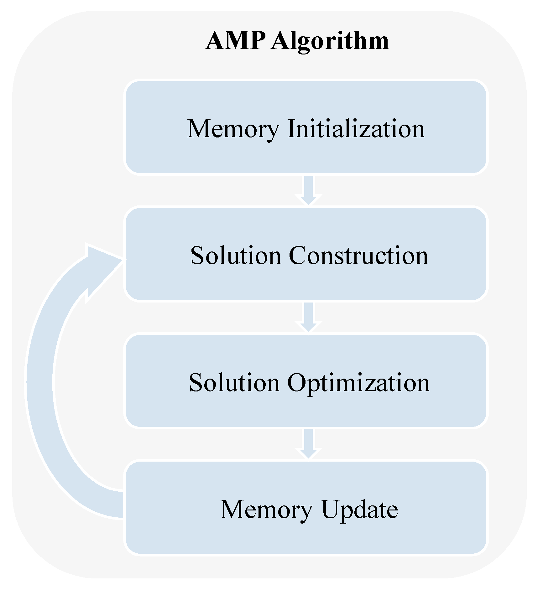
Initially, all drones are mounted on the vehicle, with identical positions and remaining endurance, forming a symmetric state. In this case, the drone flight routes can be determined first, and then these routes can be assigned to individual drones for execution. For the task nodes covered by each parking node, multiple drone flight routes need to be determined. These routes must cover all task nodes, and the drones will visit the task nodes according to these routes. In this study, we use the AMP algorithm to solve the drone flight routes at each parking node. The core idea of the AMP algorithm is that a good solution can often be constructed by combining components of other good solutions. In this context, a solution for the drone flight routes at a parking node is a set of multiple drone flight routes. By selecting and combining the best components from multiple solutions, a superior solution can be obtained. Iterating this process will eventually lead to an optimal solution. Figure 3 shows the flowchart of solving the drone flight routes at a parking node based on the AMP algorithm. The following sections will provide a detailed explanation of each part of the process for solving drone flight routes using the AMP algorithm.

(1) Memory Initialization: The algorithm begins with the initialization of the memory pool, which is designated to store the flight paths of drones. The initialization process employs a combination of random and greedy algorithms to construct multiple drone flight paths. Specifically, for a parking node $p_i$, a task node is randomly selected from the set of task nodes $C_{p_i}$ assigned to $p_i$, to serve as the initial task node in the drone flight path. Subsequently, the nearest task node to the current task node is chosen as the next node. This procedure is repeated until the length of the constructed drone flight path exceeds the drone’s maximum flight distance. The completed drone flight path is then added to the memory pool, and the task nodes contained within this flight path are removed from $C_{p_i}$. This process is repeated until all task nodes in $C_{p_i}$ have been allocated to drone flight paths. Once $C_{p_i}$ is exhausted, it is reinitialized, and the construction continues until the memory pool reaches its maximum capacity $n_{max}$. The pseudocode for the memory pool initialization is presented in Algorithm 3.

Algorithm 3 solving the drones route

Input:  parking node$p_i$, assigned task nodes set $C_{p_i}$ at $p_i$; Output:  memory pool M;  1: Initialize M and $n_{max}$;  2: while$\left|M\right|<n_{max}$do  3:    $C_{p_i}\_temp=C_{p_i}$;  4:    while $C_{p_i}\_temp\ne ⌀$ do  5:      $r=\left\{\right\}$, $dist=d_{uav}$;  6:      choose a random task node $c_j$ in $C_{p_i}\_temp$;  7:      $r\leftarrow r\bigcup \left\{c_j\right\}$, update $dist$, $c_{now}\leftarrow c_j$;  8:      while $\left|C_{p_i}\_temp\right|>0$ and $dist>0$ do  9:         get the task node $c_k$ that is closest to $c_{now}$; 10:         $c_{now}\leftarrow c_k$, update $dist$; 11:         if $dist>0$ then 12:           $r\leftarrow r\bigcup \left\{c_k\right\}$; 13:         end if 14:      end while 15:      $C_{p_i}\_temp=C_{p_i}\_temp\setminus r$; 16:    end while 17: end while 18: return M;

(2) Solution Construction: After the initialization of the memory pool, it is necessary to construct the solution for the drone flight routes at the current parking node. First, evaluate the drone flight routes in the memory pool M. Each drone flight route in memory M is evaluated using the average access distance, which is defined by Equation (17):

$$d_{avg}\left(r\right)={\displaystyle \frac{l\left(r\right)}{\left|r\right|}}$$

(17)

Here, $l\left(r\right)$ represents the length of a drone flight route in the memory pool M, and $\left|r\right|$ denotes the number of task nodes in that route.

The route with the shortest average access distance is selected to construct the solution. Subsequently, the remaining drone flight routes in the memory pool M are updated. If any of these remaining routes contain task nodes already included in the selected route, those task nodes are removed, and the average access distance for the remaining routes is recalculated. This process continues until the selected routes cover all task nodes in the region. The pseudocode for this procedure is provided in Algorithm 4.

Algorithm 4 construction of drone flight routes solution

Input:  memory pool M, parking node $p_i$ , assigned task nodes set $C_{p_i}$ at $p_i$; Output:  drone flight routes solution $R_{p_i}$ at $p_i$;  1: while$C_{p_i}\ne ⌀$do  2:    sort the drone flight paths in M according to $d_{avg}\left(r\right)$;  3:    get the drone flight path r with the smallest $d_{avg}\left(r\right)$ from the memory M;  4:    $R_{p_i}\leftarrow R_{p_i}\bigcup \left\{r\right\}$;  5:    $M^{\prime }\leftarrow M^{\prime }\setminus r$;  6:    for $c_j\in r$ do  7:      $C_{p_i}\leftarrow C_{p_i}\setminus c_j$;  8:      for $r_k\in M^{\prime }$ do  9:         if $c_j\in r_k$ then 10:           $r_k\leftarrow r_k\setminus c_j$; 11:         end if 12:      end for 13:    end for 14: end while 15: return$R_{p_i}$;

(3) Solution Optimization: After constructing the drone flight route solutions, it is necessary to optimize these routes. This paper employs a local search strategy to enhance the efficiency of the drone flight paths. Specifically, two drone flight routes, $r_1=\{\dots ,c_{i-1},c_i,c_{i+1},\dots \}$ and $r_2=\{\dots ,c_{j-1},c_j,c_{j+1},\dots \}$, are randomly selected from the solution set. The closest task nodes within these routes, $c_i$ and $c_j$, are identified. The following two operations are performed on these task nodes:

Task Node Swap: Exchange the positions of $c_i$ and $c_j$ in $r_1$ and $r_2$, resulting in the new routes $r_1^{*}=\{\dots ,c_{i-1},c_j,c_{i+1},\dots \}$ and $r_2^{*}=\{\dots ,c_{j-1},c_i,c_{j+1},\dots \}$.

Task Node Move: There are four move strategies for task node migration: ①Move $c_i$ from $r_1$ to immediately after $c_j$ in $r_2$, resulting in new routes $r_1^{*}=\{\dots ,c_{i-1},c_{i+1},\dots \}$ and $r_2^{*}=\{\dots ,c_{j-1},c_j,c_i,c_{j+1},\dots \}$. ②Move $c_i$ from $r_1$ to immediately before $c_j$ in $r_2$, resulting in new routes $r_1^{*}=\{\dots ,c_{i-1},c_{i+1},\dots \}$ and $r_2^{*}=\{\dots ,c_{j-1},c_i,c_j,c_{j+1},\dots \}$. ③Move $c_j$ from $r_2$ to immediately after $c_i$ in $r_1$, resulting in new routes $r_1^{*}=\{\dots ,c_{i-1},c_i,c_j,c_{i+1},\dots \}$ and $r_2^{*}=\{\dots ,c_{j-1},c_{j+1},\dots \}$.④Move $c_j$ from $r_2$ to immediately before $c_i$ in $r_1$, resulting in new routes $r_1^{*}=\{\dots ,c_{i-1},c_j,c_i,c_{i+1},\dots \}$ and $r_2^{*}=\{\dots ,c_{j-1},c_{j+1},\dots \}$.

Figure 4 illustrates these two operations. The pseudocode for the detailed optimization process of the drone flight route solutions is provided in Algorithm 5:

Algorithm 5 optimization of drone flight routes solution

Input:  $p_i$, $R_{p_i}$; Output:  $R_{p_i}$;  1: for$j=1toepoch$do  2:    randomly take out two drone flight paths $r_1$ and $r_2$ from $R_{p_i}$;  3:    find the two closest task nodes $c_i$ and $c_j$ in $r_1$ and $r_2$;  4:    $r^{*}=\left\{\right\}$;  5:    $(r_1^{*1},r_2^{*1})\leftarrow swap(c_i,c_j)$, $r^{*}=r^{*}\bigcup \left\{(r_1^{*1},r_2^{*1})\right\}$;  6:    $(r_1^{*2},r_2^{*2}),(r_1^{*3},r_2^{*3}),(r_1^{*4},r_2^{*4}),(r_1^{*5},r_2^{*5})\leftarrow move(c_i,c_j)$;  7:    $r^{*}=r^{*}\bigcup \{(r_1^{*2},r_2^{*2}),(r_1^{*3},r_2^{*3}),(r_1^{*4},r_2^{*4}),(r_1^{*5},r_2^{*5})\}$;  8:    for $(r_1^{*i},r_2^{*i})\in r^{*}$ do  9:      if $l\left(r_1^{*i}\right)>d_{uav}$ or $l\left(r_2^{*i}\right)>d_{uav}$ then 10:         $r^{*}=r^{*}\setminus (r_1^{*i},r_2^{*i})$; 11:      end if 12:    end for 13:    $r^{*}=r^{*}\bigcup \left\{(r_1,r_2)\right\}$; 14:    get the route group $(r_1^{shortest},r_2^{shortest})$ with the shortest sum of route lengths in $r^{*}$; 15:    if $l\left(r_1^{shortest}\right)+l\left(r_2^{shortest}\right)<l\left(r_1\right)+l\left(r_2\right)$ then 16:      replace $r_1$ and $r_2$ in $R_{p_i}$ with $r_1^{shortest}$ and $r_2^{shortest}$; 17:    end if 18: end for 19: return$R_{p_i}$;

(4) Memory Update: Following the optimization of the drone flight route solutions, a more efficient solution is obtained. The next step involves storing these optimized routes in the memory pool, enabling the construction of superior solutions in subsequent iterations. During the memory update process, if the number of drone flight routes in the memory pool reaches its maximum capacity $n_{max}$, the algorithm removes the less optimal routes, specifically those with larger $d_{avg}\left(r\right)$ values. It is crucial to ensure that the remaining routes still cover all task nodes at the current parking node before deleting the less optimal routes. If the remaining routes fail to cover all task nodes, the algorithm will select and delete other less optimal routes instead.

4.1.4. Allocating Drone Flight Routes

After determining the drone flight routes at each parking node, it is necessary to allocate these routes to specific drones. To achieve this, a greedy approach is employed for route allocation. The core idea of the algorithm is as follows: first, all drone flight routes are sorted in descending order based on their length. This step ensures that longer routes are prioritized for allocation. Then, in each allocation step, the algorithm selects the drone with the shortest total assigned route length, denoted as $t_{u_k}$, and assigns the longest unassigned drone flight route to it. This method minimizes the total completion time and achieves load balancing. The pseudocode for the drone flight route allocation process is provided in Algorithm 6.

Algorithm 6 allocating drone flight routes

Input:  $R_{p_i}$, the set of drones U; Output:  the set of drone flight routes assigned to each drone at $p_i$ $S_{p_i}$;  1: $S_{p_i}=\left\{\right\}$;  2: the set of drone flight routes assigned to each drone at $p_i$ $S_{p_i}$;  3: while$R_{p_i}\ne ⌀$do  4:    get the longest drone flight route $r_j$ in $R_{p_i}$;  5:    get the drone $u_k$ with the smallest $t_u$ in U;  6:    assign $r_j$ to $u_k$;  7:    update $t_{u_k}$;  8:    $R_{p_i}=R_{p_i}\setminus r_j$;  9: end while 10: $S_{p_i}\leftarrow$ the set of drone flight routes assigned to each drone in the U; 11: return$S_{p_i}$;

4.2. Adjusting the Current Data Collection Plan for Dynamic Task Arrivals

After allocating the drone flight routes, the initial global data collection plan is complete. At this point, the vehicle carrying the drones only needs to follow the planned vehicle route to reach each parking node sequentially, and the drones will visit the task nodes according to their assigned flight routes. When new task nodes are added during the task execution by the vehicle and drones, the current data collection plan needs to be adjusted. This adjustment involves three key steps:

(1) dividing new task nodes: New task nodes are divided into the unvisited task node set and the unplanned task node set. Task nodes in the unplanned set are initially not visited.

(2) solving local data collection plan: A local data collection plan is devised to visit the task nodes in the unvisited task node set.

(3) solving global data collection plan: When conditions during task execution warrant solving for a new global data collection plan, task nodes from the unplanned task node set are added to the unvisited task node set. A new global data collection plan is then devised for all task nodes in the unvisited set. The following sections provide a detailed explanation of each step.

4.2.1. Dividing New Task Nodes

In scenarios where tasks arrive dynamically, new task nodes may be added during the execution process. When this occurs, it is necessary to divide the task nodes accordingly. Define the area covered by the remaining unvisited parking nodes as the unvisited area ${\Omega }_{uv}$ and the remaining area as the unplanned area ${\Omega }_{up}$. Task nodes distributed within the unvisited area are defined as the unvisited task node set $C_{uv}$, while task nodes distributed within the unplanned area are defined as the unplanned task node set $C_{up}$. New task nodes will be distributed within ${\Omega }_{uv}$ and ${\Omega }_{up}$. Task nodes located in ${\Omega }_{uv}$ will be classified into $C_{uv}$, while task nodes located in ${\Omega }_{up}$ will be classified into $C_{up}$. A local data collection plan will be devised to visit the task nodes in $C_{uv}$, while the task nodes in $C_{up}$ will not be considered initially.

4.2.2. Solving Local Data Collection Plan

When tasks dynamically arrive, there are two possible states for task execution: (1) the drone is collecting data while the vehicle is stationed at a parking node; (2) all drones are on the vehicle, which is en route to the next parking node. For the first scenario, when the vehicle arrives at a new task node while parked, the current flight path of each drone must be replanned based on their current position and remaining battery life. The AMP algorithm is then employed to determine the optimal flight paths for drones from the current parking node to the remaining unvisited nodes. These paths are subsequently reassigned to each drone, forming the local data collection scheme. In the second scenario, only the AMP algorithm is required to solve the flight paths of drones for the remaining unvisited parking nodes. These paths are then reassigned to the drones, resulting in the local data collection scheme. The pseudocode for the solution process of the local data collection scheme is provided in Algorithm 7.

Algorithm 7 solving local data collection plan

Input:  the parking nodes set is not visited P, $R_P$; Output:  the set of drone flight routes assigned to each drone at parking nodes $S_P$;  1: $R_P=\{R_{p_1},R_{p_2},\dots ,R_{p_{\left|P\right|}}\}$, $S_P=\{S_{p_1},S_{p_2},\dots ,S_{p_{\left|P\right|}}\}$;  2: if vehicle is parking at the parking node then  3:    get the parking node $p_{now}$;  4:    $P\leftarrow P/p_{now}$;  5:    $R_{p_{now}}\leftarrow$ call Algorithm 8 + AMP Algorithm;  6:    $S_{p_{now}}\leftarrow$ call Algorithm 6;  7: end if  8: for$p_i\in P$do  9:    $R_{p_1}\leftarrow$ AMP Algorithm; 10:    $S_{p_i}\leftarrow$ call Algorithm 6; 11: end for 12: return$S_P$;

When tasks dynamically arrive and drones are executing tasks, new task nodes may appear within the coverage area of the parking node where the drones are stationed. At this time, since each drone has a different position and remaining endurance, forming an asymmetric state, it is necessary to re-plan the flight route for each drone to maximize flight benefits based on its current position, remaining endurance, and newly added task nodes. For the current parking node $p_i$, let $E_{p_i}$ denote the set of remaining unvisited task nodes at $p_i$. The algorithm first calculates the current position and remaining battery life of each drone. Then, it selects the task node from $E_{p_i}$ that is closest to all drones. The algorithm assigns this task node to the nearest drone and checks whether the drone can successfully return after completing the task. If the drone can return, the task node is assigned to it, and the drone’s position is updated. If the drone cannot return, its remaining battery life is set to zero. This process is repeated until all drones have no remaining battery life or $E_{p_i}$ is empty. This constructs the current flight paths for all drones. The pseudocode for the process of adjusting the current flight paths of drones is shown in Algorithm 8.

Algorithm 8 adjusting current drone flight routes

Input:  parking node $p_i$, $E_{p_i}$, U, the location and remaining endurance of each drone; Output:  U;  1: for$u_j\in U$do  2:    $r_{p_i}^j=\left\{\right\}$;  3: end for  4: while the remaining endurance of each drone is not 0 and $E_{p_i}\ne ⌀$ do  5:    find the pair consisting of the closest drone $u_j$ from set U and task node $c_k$ from set $E_{p_i}$;  6:    if $u_j$ can return to the vehicle after visiting $c_j$ then  7:      $r_{p_i}^j=r_{p_i}^j\bigcup \left\{c_k\right\}$;  8:      $S_{p_i}=S_{p_i}\setminus c_j$;  9:      update the location and remaining endurance of $u_j$; 10:    else 11:      update $u_j$’s remaining endurance to 0; 12:    end if 13: end while 14: return U;

4.2.3. Solving Global Data Collection Plan

During the execution of the local data collection scheme, the number of task nodes in the unvisited task node set $C_{uv}$ gradually decreases. When the number of task nodes in the unplanned task node set $C_{up}$ is smaller than that in $C_{uv}$, the number of task nodes in the unplanned region ${\Omega }_{up}$ is too few, resulting in high time costs for visitation. At this point, the task nodes in $C_{up}$ are temporarily disregarded. However, when the number of task nodes in $C_{up}$ is greater than or equal to that in $C_{uv}$, there are sufficient task nodes distributed in the unplanned region ${\Omega }_{up}$. In this case, a global data collection scheme needs to be devised to visit the task nodes in both $C_{uv}$ and $C_{up}$. It is important to note that the vehicle route in the global data collection scheme is not a closed-loop route. Therefore, the Ant Colony Algorithm cannot be used for solving it. Instead, a greedy strategy is employed to determine the vehicle’s route, selecting the nearest unvisited parking node from the current position as the next stop. The pseudocode for solving the global data collection scheme is shown in Algorithm 9.

Algorithm 9 solving global data collection plan

Input:  $C_{uv}$, $C_{up}$, A; Output:  $r_{truck}$, $S_P$; 1: $P=\left\{\right\}$, $C_P=\left\{\right\}$, $r_{truck}=\left\{\right\}$, $R_P=\{R_{p_1},R_{p2},\dots ,R_{p_{\left|P\right|}}\}$, $S_P=\{S_{p_1},S_{p_2},\dots ,S_{p_{\left|P\right|}}\}$; 2: $C_{uv}\leftarrow C_{uv}\bigcup C_{up}$; 3: P, $C_P\leftarrow$call Algorithm 1; 4: $r_{truck}\leftarrow$ use the greedy algorithm to solve the vehicle route; 5: for$p_i\in P$do 6:    $R_{p_i}\leftarrow$ AMP Algorithm; 7:    $S_{p_1}\leftarrow$ call Algorithm 6; 8: end for 9: return$r_{truck}$, $S_P$;

5. Experiments

To comprehensively evaluate the performance of GAMPDA, extensive simulation experiments were conducted in this chapter. We compared GAMPDA with three other algorithms: (1) the SCAN algorithm (SCAN); (2) the God’s Perspective algorithm (GP); and (3) the LKH algorithm (LKH). The SCAN algorithm does not dynamically replan routes upon the arrival of new task batches. Instead, it plans routes for these new task nodes only after all batches have arrived, ensuring that the drones and vehicle complete all static initial tasks before addressing the new task nodes. The GP assumes that all task node information, including future dynamically arriving task batches, is known in advance, so the result of the GP is the ideal outcome. The LKH solver is a heuristic approach that can quickly provide near-optimal solutions. To utilize the LKH for this problem, we convert it into a traveling salesman problem (TSP). We assume that all task nodes are visited by a vehicle for data collection. The vehicle starts from a start node, travels to each task node within the designated area, and then returns to the start node.

The evaluation metrics include time cost, vehicle travel distance, and drone flight distance. The time cost refers to the total task execution time of the entire system, measured from the moment the drones and trunk receive the route from the central console and depart from the starting node $n_0$ until the trunk, carrying the drones, returns to $n_0$ after completing the final task node. The vehicle travel distance is the total distance traveled by the vehicle from $n_0$ to its return to $n_0$. The drone flight distance is the total length of the flight routes of the $\left|U\right|$ drones. Among these, the time cost is the primary metric, while the vehicle travel distance and drone flight distance are secondary metrics.

The default experimental parameters are set as shown in

Table 2. Default settings of relative parameters.

Parameter	Value
The side length of the target area	50 km
The initial number of task nodes	2000
The number of vehicles	1
The number of drones	3
The speed of the vehicle	15 m/s
The speed of the drone	10 m/s
The maximum endurance of the drone	15 km
The dynamic task arrival interval	8 h
The maximum number of arrival batches	4

. The total number of dynamically arriving task nodes is equal to the initial task nodes, and each batch of dynamically arriving tasks equals the total number of initial tasks divided by the number of batches, and the dynamically arriving tasks are randomly distributed within the target area. Therefore, the arrival of task nodes is symmetric. Based on these default experimental parameters, this paper primarily investigates the impact of the number of initial task nodes, the size of the target area, and the number of drones on the algorithm’s performance.

To observe the impact of varying the number of task nodes on the algorithm’s performance, the number of task nodes is set to vary within the range [1500, 2300], while keeping other parameters at their default values.

In Figure 5, as the number of task nodes increases, the time cost for all four algorithms increases linearly. The lowest time cost is observed with the GP, followed closely by GAMPDA, which performs significantly better than SCAN and LKH. SCAN, due to the lack of dynamic route planning, performs worse than GAMPDA. The LKH shows the poorest performance, indicating that regardless of whether a dynamic algorithm is used, a single vehicle is far less efficient compared to the collaborative mechanism of multiple drones and trunks.

In Figure 6, it can be seen that the vehicle travel distance remains relatively stable as the number of task nodes varies. This is because the vehicle route consists of parking nodes, and an increase in the number of task nodes does not lead to a linear increase in the number of parking nodes. Therefore, the length of the vehicle route does not increase significantly. The comparison of the four algorithms shows that GAMPDA, SCAN, and GP have similar results, with GAMPDA performing slightly better than SCAN. The LKH performs poorly, with an abnormally high vehicle travel distance because it relies on a single vehicle to visit all task nodes, whereas the other three algorithms only require the vehicle to reach some parking nodes, saving a significant amount of time and distance.

In Figure 7, as the number of task nodes increases, the drone flight distance for all three algorithms increases linearly. The drone flight distance for GAMPDA is less than that for SCAN, indicating better performance. Additionally, the trend in the drone flight distance is consistent with the time cost, suggesting that the algorithm’s performance is mainly influenced by drone route planning. This aligns with the algorithm logic, as all task nodes are visited by drones, with the vehicle only needing to reach several parking nodes.

The number of task nodes is set to the default value of 2000, while the size of the target area is varied, with the side length ranging from [30, 70] km to observe the algorithm’s performance.

In Figure 8, the time cost for all algorithms except SCAN shows a linear increase as the side length of the area grows. DTAPA’s performance is closest to the GP, followed by SCAN, with the LKH performing the worst. When the side length increases to 60 km and 70 km, the time cost of SCAN surpasses that of the LKH. This is because SCAN does not handle new tasks immediately; instead, it completes all previous tasks before returning to execute new tasks. Consequently, SCAN requires multiple round trips. As the side length increases, the time cost of SCAN grows increasingly faster due to these multiple trips, deviating from a linear relationship.

In Figure 9, the vehicle travel distance in the LKH increases linearly with the side length of the area, as the vehicle undertakes all visitation tasks, and the larger map results in a linear increase in the distance to visit task nodes. The other three algorithms show only slight increases, indicating that changes in the area side length have minimal impact on the vehicle travel distance for GAMPDA, SCAN, and GP. As the side length increases, the distance between parking nodes might slightly increase, leading to a slight increase in vehicle travel distance. Among these, GAMPDA remains closest to the GP in performance.

In Figure 10, the curves for GAMPDA and GP are almost parallel, indicating similar growth trends. However, SCAN’s curve has a steeper slope. This is because in SCAN, drones return to execute newly arrived tasks after completing existing ones, making the drone flight distance significantly affected by the increase in area side length.

This study examines the collaborative node inspection problem involving multiple drones and a vehicle, making the number of drones a crucial factor affecting the algorithm’s performance. Since the LKH involves only the vehicle and no drones, its results are not included in this figure.

In Figure 11, as the number of drones increases, the time cost for all three algorithms decreases, albeit at a diminishing rate. GAMPDA has a time cost approximately 13% lower than SCAN. However, as the number of drones continues to increase, the time cost will no longer decrease. This is because the existing drones are already sufficient to handle the 2000 task nodes within the target area, reaching performance saturation.

In Figure 12, the number of drones only affects the task collection time within parking nodes and does not influence the clustering and selection of docking parking nodes. Therefore, the vehicle travel route remains unaffected by changes in the number of drones. The experimental results also show that the vehicle travel distance curves for the three algorithms are nearly independent of the number of drones.

In Figure 13, increasing the number of drones does not significantly change the curves for SCAN and GP. The number of drones does not affect the drone route planning, so the drone flight distance remains unchanged. However, in the dynamic GAMPDA, an increase in the number of drones allows for faster completion of initial static task nodes, rapidly expanding the visited area. Consequently, more newly arriving task nodes fall within the visited area. Note that the density of new task nodes within the expanded visited area remains low, maintaining a low-density distribution. When the number of new task nodes in the visited area exceeds those in the unvisited but planned areas, global optimization is triggered earlier. Therefore, an increase in the number of drones indirectly leads to earlier global optimization. To execute tasks in the newly visited area, the vehicle must return to this area for drone route planning. Due to the low density of new task nodes, the length of the drone routes will increase. Hence, the conclusion can be drawn that increasing the number of drones indirectly leads to earlier global optimization, which in turn increases the total drone flight distance.

6. Conclusions

This paper investigates the problem of data collection in a scenario with dynamically arriving tasks, where vehicle and drones collaborate. The problem is formulated as a 0–1 integer programming model, and an effective framework is provided to optimize the data collection process while considering the constraints and requirements of both the vehicle and drones. To solve this problem, we propose the GAMPDA optimization algorithm, which can dynamically adjust the data collection plan in real time to minimize the overall task completion time. Simulation experiments validate the feasibility and effectiveness of GAMPDA. Future research will consider additional dynamic factors, such as weather conditions and drone malfunctions, which may further impact the performance and robustness of the data collection process. Incorporating these factors will enhance the algorithm’s adaptability, making it more suitable for real-world applications.

References

1. Ma, X.; Yao, T.; Hu, M.; Dong, Y.; Liu, W.; Wang, F.; Liu, J. A Survey on Deep Learning Empowered IoT Applications. IEEE Access 2019, 7, 181721–181732. [Google Scholar] [CrossRef]
2. Hu, M.; Li, J.; Cai, C.; Deng, T.; Xu, W.; Dong, Y. Software Defined Multicast for Large-Scale Multi-Layer LEO Satellite Networks. IEEE Trans. Netw. Serv. Manag. 2022, 19, 2119–2130. [Google Scholar] [CrossRef]
3. Hu, M.; Luo, J.; Wang, Y.; Lukasiewycz, M.; Zeng, Z. Holistic Scheduling of Real-Time Applications in Time-Triggered In-Vehicle Networks. IEEE Trans. Ind. Inform. 2014, 10, 1817–1828. [Google Scholar] [CrossRef]
4. Cai, C.; Pu, H.; Hu, M.; Zheng, R.; Luo, J. Acoustic Software Defined Platform: A Versatile Sensing and General Benchmarking Platform. IEEE Trans. Mob. Comput. 2023, 22, 647–660. [Google Scholar] [CrossRef]
5. Hu, M.; Luo, J.; Wang, Y.; Veeravalli, B. Practical Resource Provisioning and Caching with Dynamic Resilience for Cloud-Based Content Distribution Networks. IEEE Trans. Parallel Distrib. Syst. 2014, 25, 2169–2179. [Google Scholar] [CrossRef]
6. Das, D.N.; Sewani, R.; Wang, J.; Tiwari, M.K. Synchronized truck and drone routing in package delivery logistics. IEEE Trans. Intell. Transp. Syst. 2020, 22, 5772–5782. [Google Scholar] [CrossRef]
7. Lemardelé, C.; Estrada, M.; Pagès, L.; Bachofner, M. Potentialities of drones and ground autonomous delivery devices for last-mile logistics. Transp. Res. Part E Logist. Transp. Rev. 2021, 149, 102325. [Google Scholar] [CrossRef]
8. Nycz, B.; Pietrucha-Urbanik, K. Advancements in Air Quality Monitoring: The Role of Drone Technology. Proceedings 2024, 105, 19. [Google Scholar] [CrossRef]
9. Baumgart, J.; Mikołajewski, D.; Czerniak, J.M. Taking Flight for a Greener Planet: How Swarming Could Help Monitor Air Pollution Sources. Electronics 2024, 13, 577. [Google Scholar] [CrossRef]
10. Wang, Q.; Zhang, J.; Lei, M.; Li, H.; Peng, K.; Hu, M. Toward Wide Area Remote Sensor Calibrations: Applications and Approaches. IEEE Sensors J. 2024, 24, 8991–9001. [Google Scholar] [CrossRef]
11. Peng, K.; Wang, L.; He, J.; Cai, C.; Hu, M. Joint Optimization of Service Deployment and Request Routing for Microservices in Mobile Edge Computing. IEEE Trans. Serv. Comput. 2024, 17, 1016–1028. [Google Scholar] [CrossRef]
12. da Silva, R.I.; Rezende, J.D.C.V.; Souza, M.J.F. Collecting large volume data from wireless sensor network by drone. Ad Hoc Netw. 2023, 138, 103017. [Google Scholar] [CrossRef]
13. Liu, Y.; Li, X.; He, B.; Gu, M.; Huangfu, W. UAV-Enabled Diverse Data Collection via Integrated Sensing and Communication Functions Based on Deep Reinforcement Learning. Drones 2024, 8, 647. [Google Scholar] [CrossRef]
14. Hu, M.; Liu, W.; Lu, J.; Fu, R.; Peng, K.; Ma, X.; Liu, J. On the joint design of routing and scheduling for vehicle-assisted multi-UAV inspection. Future Gener. Comput. Syst. 2019, 94, 214–223. [Google Scholar] [CrossRef]
15. Wang, D.; Hu, P.; Du, J.; Zhou, P.; Deng, T.; Hu, M. Routing and Scheduling for Hybrid Truck-Drone Collaborative Parcel Delivery With Independent and Truck-Carried Drones. IEEE Internet Things J. 2019, 6, 10483–10495. [Google Scholar] [CrossRef]
16. El-Adle, A.M.; Ghoniem, A.; Haouari, M. Parcel delivery by vehicle and drone. J. Oper. Res. Soc. 2021, 72, 398–416. [Google Scholar] [CrossRef]
17. Zhang, J.; Li, Y. Collaborative vehicle-drone distribution network optimization for perishable products in the epidemic situation. Comput. Oper. Res. 2023, 149, 106039. [Google Scholar] [CrossRef]
18. Mara, S.T.W.; Sarker, R.; Essam, D.; Elsayed, S. Solving electric vehicle–drone routing problem using memetic algorithm. Swarm Evol. Comput. 2023, 79, 101295. [Google Scholar] [CrossRef]
19. Karak, A.; Abdelghany, K. The hybrid vehicle-drone routing problem for pick-up and delivery services. Transp. Res. Part C Emerg. Technol. 2019, 102, 427–449. [Google Scholar] [CrossRef]
20. Murray, C.C.; Chu, A.G. The flying sidekick traveling salesman problem: Optimization of drone-assisted parcel delivery. Transp. Res. Part C Emerg. Technol. 2015, 54, 86–109. [Google Scholar] [CrossRef]
21. Agatz, N.; Bouman, P.; Schmidt, M. Optimization approaches for the traveling salesman problem with drone. Transp. Sci. 2018, 52, 965–981. [Google Scholar] [CrossRef]
22. Ha, Q.M.; Deville, Y.; Pham, Q.D.; Hà, M.H. On the min-cost traveling salesman problem with drone. Transp. Res. Part C Emerg. Technol. 2018, 86, 597–621. [Google Scholar] [CrossRef]
23. Salama, M.; Srinivas, S. Joint optimization of customer location clustering and drone-based routing for last-mile deliveries. Transp. Res. Part C Emerg. Technol. 2020, 114, 620–642. [Google Scholar] [CrossRef]
24. Kang, M.; Lee, C. An exact algorithm for heterogeneous drone-truck routing problem. Transp. Sci. 2021, 55, 1088–1112. [Google Scholar] [CrossRef]
25. Chang, Y.S.; Lee, H.J. Optimal delivery routing with wider drone-delivery areas along a shorter truck-route. Expert Syst. Appl. 2018, 104, 307–317. [Google Scholar] [CrossRef]
26. Peng, K.; Liu, W.; Sun, Q.; Ma, X.; Hu, M.; Wang, D.; Liu, J. Wide-Area Vehicle-Drone Cooperative Sensing: Opportunities and Approaches. IEEE Access 2019, 7, 1818–1828. [Google Scholar] [CrossRef]
27. Hu, M.; Liu, W.; Peng, K.; Ma, X.; Cheng, W.; Liu, J.; Li, B. Joint Routing and Scheduling for Vehicle-Assisted Multidrone Surveillance. IEEE Internet Things J. 2019, 6, 1781–1790. [Google Scholar] [CrossRef]
28. Peng, K.; Du, J.; Lu, F.; Sun, Q.; Dong, Y.; Zhou, P.; Hu, M. A Hybrid Genetic Algorithm on Routing and Scheduling for Vehicle-Assisted Multi-Drone Parcel Delivery. IEEE Access 2019, 7, 49191–49200. [Google Scholar] [CrossRef]
29. Wang, Z.; Sheu, J.B. Vehicle routing problem with drones. Transp. Res. Part B Methodol. 2019, 122, 350–364. [Google Scholar] [CrossRef]
30. Deng, T.; Xu, X.; Zou, Z.; Liu, W.; Wang, D.; Hu, M. Multidrone Parcel Delivery via Public Vehicles: A Joint Optimization Approach. IEEE Internet Things J. 2024, 11, 9312–9323. [Google Scholar] [CrossRef]
31. Luo, Z.; Liu, Z.; Shi, J. A Two-Echelon Cooperated Routing Problem for a Ground Vehicle and Its Carried Unmanned Aerial Vehicle. Sensors 2017, 17, 1144. [Google Scholar] [CrossRef] [PubMed]
32. Sacramento, D.; Pisinger, D.; Ropke, S. An adaptive large neighborhood search metaheuristic for the vehicle routing problem with drones. Transp. Res. Part C Emerg. Technol. 2019, 102, 289–315. [Google Scholar] [CrossRef]
33. Liu, Y.; Luo, Z.; Liu, Z.; Shi, J.; Cheng, G. Cooperative Routing Problem for Ground Vehicle and Unmanned Aerial Vehicle: The Application on Intelligence, Surveillance, and Reconnaissance Missions. IEEE Access 2019, 7, 63504–63518. [Google Scholar] [CrossRef]
34. Campuzano, G.; Lalla-Ruiz, E.; Mes, M. The drone-assisted variable speed asymmetric traveling salesman problem. Comput. Ind. Eng. 2023, 176, 109003. [Google Scholar] [CrossRef]
35. Liu, Z.; Li, X.; Khojandi, A. The flying sidekick traveling salesman problem with stochastic travel time: A reinforcement learning approach. Transp. Res. Part E Logist. Transp. Rev. 2022, 164, 102816. [Google Scholar] [CrossRef]
36. Murray, C.C.; Raj, R. The multiple flying sidekicks traveling salesman problem: Parcel delivery with multiple drones. Transp. Res. Part C Emerg. Technol. 2020, 110, 368–398. [Google Scholar] [CrossRef]
37. Arishi, A.; Krishnan, K.; Arishi, M. Machine learning approach for truck-drones based last-mile delivery in the era of industry 4.0. Eng. Appl. Artif. Intell. 2022, 116, 105439. [Google Scholar] [CrossRef]
38. Moshref-Javadi, M.; Lee, S.; Winkenbach, M. Design and evaluation of a multi-trip delivery model with truck and drones. Transp. Res. Part E Logist. Transp. Rev. 2020, 136, 101887. [Google Scholar] [CrossRef]
39. Kloster, K.; Moeini, M.; Vigo, D.; Wendt, O. The multiple traveling salesman problem in presence of drone-and robot-supported packet stations. Eur. J. Oper. Res. 2023, 305, 630–643. [Google Scholar] [CrossRef]
40. Zou, B.; Wu, S.; Gong, Y.; Yuan, Z.; Shi, Y. Delivery network design of a locker-drone delivery system. Int. J. Prod. Res. 2024, 62, 4097–4121. [Google Scholar] [CrossRef]
41. Wu, Y.; Low, K.H. An Adaptive Path Replanning Method for Coordinated Operations of Drone in Dynamic Urban Environments. IEEE Syst. J. 2021, 15, 4600–4611. [Google Scholar] [CrossRef]
42. Lin, I.C.; Lin, T.H.; Chang, S.H. A decision system for routing problems and rescheduling issues using unmanned aerial vehicles. Appl. Sci. 2022, 12, 6140. [Google Scholar] [CrossRef]
43. Dayarian, I.; Savelsbergh, M.; Clarke, J.P. Same-day delivery with drone resupply. Transp. Sci. 2020, 54, 229–249. [Google Scholar] [CrossRef]
44. Han, J.; Liu, Y.; Li, Y. Vehicle Routing Problem with Drones Considering Time Windows and Dynamic Demand. Appl. Sci. 2023, 13, 13086. [Google Scholar] [CrossRef]
45. Colorni, A.; Dorigo, M.; Maniezzo, V.; Trubian, M. Ant system for job-shop scheduling. JORBEL-Belg. J. Oper. Res. Stat. Comput. Sci. 1994, 34, 39–53. [Google Scholar]
Figure 1. Process of data collection through multi-drone and vehicle collaboration.
Symmetry 17 00067 g001
Figure 2. Flowchart of GAMPDA.
Symmetry 17 00067 g002
Figure 3. Flowchart of the AMP algorithm.
Symmetry 17 00067 g003
Figure 4. Schematic diagram of task node swapping and moving (The blue route and the red route represent two separate drone flight paths, respectively).
Symmetry 17 00067 g004
Figure 5. Impact of time cost with the number of task nodes.
Symmetry 17 00067 g005
Figure 6. Impact of vehicle travel distance with the number of task nodes.
Symmetry 17 00067 g006
Figure 7. Impact of drones flight distance with the number of task nodes.
Symmetry 17 00067 g007
Figure 8. Impact of time cost with the size of target area.
Symmetry 17 00067 g008
Figure 9. Impact of vehicle travel distance with the size of target area.
Symmetry 17 00067 g009
Figure 10. Impact of drones flight distance with the size of target area.
Symmetry 17 00067 g010
Figure 11. Impact of time cost with the number of drones.
Symmetry 17 00067 g011
Figure 12. Impact of vehicle travel distance with the number of drones.
Symmetry 17 00067 g012
Figure 13. Impact of drones flight distance with the number of drones.
Symmetry 17 00067 g013